Article

Development and Analysis of a Multi-Node Dynamic Model for the Simulation of Stratified Thermal Energy Storage

1
CIDEA—Center for Energy and Environment, University of Parma, Parco Area delle Scienze 42/a, 43125 Parma, Italy
2
Department of Engineering and Architecture, University of Parma, Parco Area delle Scienze 181/a, 43125 Parma, Italy
*
Author to whom correspondence should be addressed.
Energies 2019, 12(22), 4275; https://doi.org/10.3390/en12224275
Submission received: 24 September 2019 / Revised: 18 October 2019 / Accepted: 7 November 2019 / Published: 9 November 2019
(This article belongs to the Special Issue Mathematical Modelling of Energy Systems and Fluid Machinery)

Abstract

:
To overcome non-programmability issues that limit the market penetration of renewable energies, the use of thermal energy storage has become more and more significant in several applications where there is a need for decoupling between energy supply and demand. The aim of this paper is to present a multi-node physics-based model for the simulation of stratified thermal energy storage, which allows the required level of detail in temperature vertical distribution to be varied simply by choosing the number of nodes and their relative dimensions. Thanks to the chosen causality structure, this model can be implemented into a library of components for the dynamic simulation of smart energy systems. Hence, unlike most of the solutions proposed in the literature, thermal energy storage can be considered not only as a stand-alone component, but also as an important part of a more complex system. Moreover, the model behavior has been analyzed with reference to the experimental results from the literature. The results make it possible to conclude that the model is able to accurately predict the temperature distribution within a stratified storage tank typically used in a district heating network with limitations when dealing with small storage volumes and high flow rates.

Graphical Abstract

1. Introduction

The continuous increase in the importance of the role of energy over the last few decades, as well as the rise in fuel prices and the need to limit greenhouse gas emissions, have led to a steady growth in the use of energy saving technologies and in a more effective and extensive implementation of renewable energy sources [1]. However, despite renewable energies representing one of the best alternatives to conventional sources—such as fossil or nuclear—for energy supply in most areas of the world, renewable energies are often hampered by their discontinuous nature during the day and by the actual availability of the source during the year.
As a matter of fact, energy is not always available where, when, and how it is required, and thus storage systems (both electrical and thermal) play an important role in energy management to make it available accordingly. Therefore, to improve the availability of renewable energies in remote geographical areas and to overcome their intermittent nature, thermal energy storage (TES) represents a fundamental solution to increase their competitiveness. Thanks to its capability to allow a more sustainable use of available resources [2] and to decouple thermal energy generation and use, there is currently growing interest in thermal energy storage.
A number of applications for thermal energy storage can be seen in energy grids, since they allow (i) an effective balance in energy supply vs. demand dynamics, (ii) a decrease in heating system energy losses, reducing the number of start-up and shut-down maneuvers and the need for backup plants, (iii) an increase in deliverable capacity (heating element generation plus storage capacity), (iv) a shift in energy purchases to lower cost periods, and (v) an increase in renewable energy source exploitation.
As an example, Barbieri et al. [3] showed the storage capability to decouple electrical and thermal power production in cogeneration plants, allowing thermal energy to be stored when only the electric energy is needed and vice-versa. It is therefore apparent that thermal energy storage represents a key solution in all applications in which energy supply and demand are decoupled, giving significant advantages in terms of cost and dispatchability of the generated energy. It can also be used to support generation by conventional energy sources [4] to deal with weekly, monthly, and annual changes in energy requirements and to help peak shaving [5]. Moreover, thermal energy storage represents a fundamental technique for the optimization of overall energy conversion, transmission, and utilization processes in smart energy systems [6]. Ultimately, it has a fundamental role in energy system control strategy development [7], such as Model-in-the-Loop applications, and implementation [8,9].
Several solutions have been proposed in the literature for thermal energy storage (e.g., through sensible heat, latent heat, and thermochemical energy) [10,11] involving the most recent areas of investigation and experimentation. A detailed analysis and a performance comparison of the existing thermal energy storage systems have been performed by Sarbu and Sebarchievici [12]. Furthermore, Noro et al. [13] focused their attention on the liquid sensible and phase change material heat storage systems, pointing out their respective pros and cons. However, because of the limitations and drawbacks of latent heat and thermochemical storage solutions—e.g., large volume variations and high storage medium costs, respectively—water is still the most widely diffused energy storage material since it is easily available, cheap, non-toxic, non-flammable, and completely harmless [14]. For these reasons, this study focuses on water sensible thermal energy storage.
A multi-node model has been developed, and the effects of node number and flow rate variations have been investigated alternatively. The model has been developed with a modular approach, by considering a standardized input/output causality structure for easy implementation into a library of components for the dynamic simulation of smart energy systems [6]. Unlike other simulation tools that are currently available [15,16], the present paper shows all the fundamental equations and their implementation in an explicit way allowing easy replicability and providing high-level customization features for both discretization and numerosity of inlet or outlet ports. Then the storage model behavior has been analyzed in charge and discharge conditions, taking the experimental data from the literature as a benchmark (i.e., the experimental model developed by González-Altozano et al. [17] and the experimental study carried out by Li et al. [18], respectively). Finally, the model has been applied to a real case in an operating environment.

Literature Review

Accurate surveys of mathematical simulation models of TES tanks were conducted by Njoku et al. [19], and Dumont et al. [20]. It follows that these models can be divided into three main categories:
  • 0D models, comprising analytical and fully-mixed approaches;
  • 1D models, including moving boundary, plug-flow and multi-node models;
  • 2D-3D models, containing multi-zone models and CFD techniques.
Starting from the 0D models, following the analytical approach, the storage tank can be modeled as a semi-infinite body, assuming that the inlet temperature and the mass flow rates are constant and not considering mixing or ambient heat losses. It should be noted that some attempts to relax these assumptions have been successfully performed in [21,22]. The fully-mixed hypothesis is still the simplest approach, since uniform temperature distribution is considered in the whole tank volume, assuming that all the incoming water mixes perfectly with the water already in the tank. Governing equations are based on mass and energy conservation [23].
Among the 1D models, the two-zone moving boundary approach is based on the assumption that the storage volume is divided into two zones with uniform temperature separated by a thermocline to prevent the hot and cold fluid from mixing and to maintain a stable temperature gradient [24]. In order to reduce the mathematical complexity of the analytical solutions, for the sake of practicability, an integral approximate approach has been successfully applied to the 1D storage tank models by Chung and Shin [25]. In the plug-flow method the tank volume is composed of a variable number of isothermal disks moving within the tank without any mixing between them [26]. Finally, the multi-node models are developed following a 1D finite-volume method that considers a uniform horizontal temperature in each layer (called a node). Therefore, a temperature gradient in the vertical direction only (i.e., stratification) and a 1D flow inside the tank [27,28] can be modeled. Using this 1D approach, González-Altozano et al. [17] have proposed a new methodology for the estimation of numerous temperature-dependent indices employed for the characterization of thermal stratification in water storage tanks (as temperature profile and thermocline thickness) during the charging phase, while Li et al. [18] have investigated the influence of several inlet structures on the stratification effectiveness and discharging performance of a tank.
Within the 2D-3D models, the zonal approach is a 3D finite-volume method with a coarse mesh based on mass and energy balances [29], instead the CFD [30,31] is a finite element method governed by mass, energy, and momentum conservation laws.
Each approach shows advantages and disadvantages depending on its specific application: the pros and cons of each model category are briefly summarized in Table 1. It is shown that the 2D-3D models allow for a more detailed simulation of physical systems compared to the 1D models, but with a higher computational burden because of the increase in dynamic states (resulting in a larger number of differential equations to be solved). Concerning the comparison between the reliability of different models, an insightful numerical study has been proposed by Cabelli [32], which states that, under particular circumstances, the temperature profile of the stratified fluid can be reasonably predicted with a simpler 1D model instead of a 2D model. Thus, in this paper specific attention has been paid to 1D models as they represent the best compromise between accuracy (which is related to the number of differential equations representing the model) and computational time (Table 1).
It is widely known that several physical phenomena occur in a water storage system that affect its performance. Among them, stratification has particularly raised the interest of researchers [27,28,33] for its strong influence on the thermal performance of plants [34,35].
For instance, Van Koppen et al. [36] and Furbo and Mikkelsen [37] found that thermal stratification in solar heating systems allows a reduction in temperature at the collector inlet (which increases its efficiency) and leads to a limited operation of the auxiliary energy supply. Accordingly, stratification improves not only the water tank efficiency, but also that of the whole extended system.
Taking into account the scope of this work, the 1D approach has been chosen by focusing the attention on multi-node architecture. Even though several approaches for multi-node modeling of thermal energy storage tanks have been proposed in the literature (as reported above), in general they do not allow variations in the number and size of nodes considered in the simulation. To allow for a more flexible customization, a new multi-node model has been developed by the authors and is presented in this paper. Both the dimensions and number of nodes of the model can be set, focusing on the desired zone of the tank, by increasing the number of nodes in that specific area.

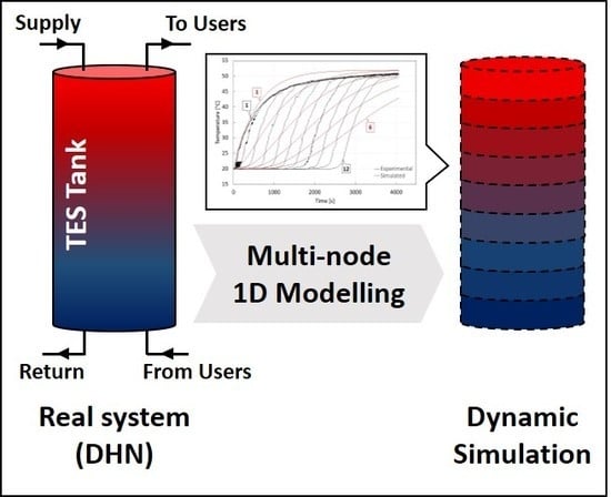
2. Materials and Methods

The model of the thermal energy storage developed by the authors falls under the multi-node 1D model category. The basic approach consists of dividing the tank into a number N of zones (called “nodes”) where temperature is considered uniform (Ti). This assumption considers the vertical gradient of the temperature in the tank, while the horizontal gradient is neglected. When numbering the nodes from the top of the tank (Figure 1), the first node is the hottest and node “N” is the last and coldest.
As the developed model is physics-based, the involved equations arise from volume (1) and energy balances (2). Thus, the continuity equation and energy conservation equation are implemented for each node in the following form:
dV dt = V ˙ ( t ) = 0
dE dt = h ( t ) · m ˙ ( t ) + Q ˙
The energy Equation (2) involves enthalpy flows and heat exchanges not related to mass flows. The latter are due to heat transfer inside the tank between neighboring nodes, and to ambient losses through the tank walls because of temperature differences between the storage medium, tank walls, and the surrounding environment. The continuity and energy balance equations are implemented for each node, considering enthalpy flows, heat transfers between adjacent nodes and ambient losses. A schematic representation of the generic node is shown in Figure 2. The governing dynamic equations for the ith node are ordinary differential equations representing volume (3) and energy balances (4):
V ˙ vert out = m ˙ in ρ ( T in ) + V ˙ vert in m ˙ out ρ ( T i )
M · c · dT i dt = m ˙ in · c · T in m ˙ out · c · T i V ˙ vert out · ρ ( T vert out ) · c · T vert out + V ˙ vert in · ρ ( T vert in ) · c · T vert in + k · ( T i 1 T i ) k · ( T i T i + 1 ) U · A · ( T i T amb )
The water density varies with the temperature, and it is thus assumed constant in each node. It must also be specified that V ˙ vert in and V ˙ vert out are positive when water is flowing downwards. Accordingly, the sign of T vert in and T vert out is defined by the following relationships:
T vert out = { T i if V ˙ vert out > 0 T i + 1 if V ˙ vert out < 0
T vert in = { T i 1 if V ˙ vert in > 0 T i if V ˙ vert in < 0
The energy conservation equation was applied to each node in order to predict its time-temperature history taking into account the thermal losses both to the surroundings and to adjacent nodes because of the convection and conduction. The latter is represented in Equation (4) by the terms k · ( T i 1 T i ) and k · ( T i T i + 1 ) , which can be appointed as “pseudo-conduction terms” since they are used to represent the thermal exchange that would take place between bordering nodes by convection.
This is a simplified way to consider these contributions (as suggested in [17,28]), but it has been noted by a preliminary analysis, which is not reported herein for the sake of brevity, that their influence on the global energy balance could be neglected. For this reason, this is an approach which is commonly used when dealing with multi-node models [15,16]. The terms V ˙ vert out · ρ ( T vert out ) · c · T vert out and V ˙ vert in · ρ ( T vert in ) · c · T vert in represent the energy associated with the incoming and outgoing flows among neighboring nodes and can be considered as “transport terms.”

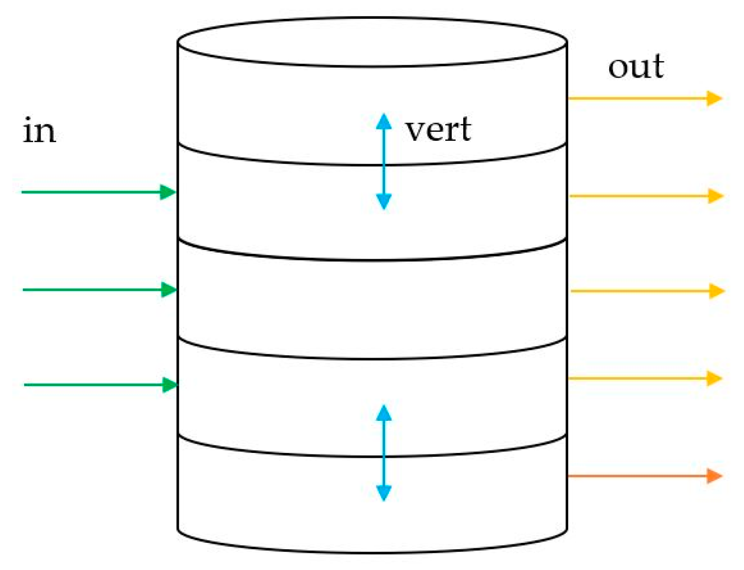
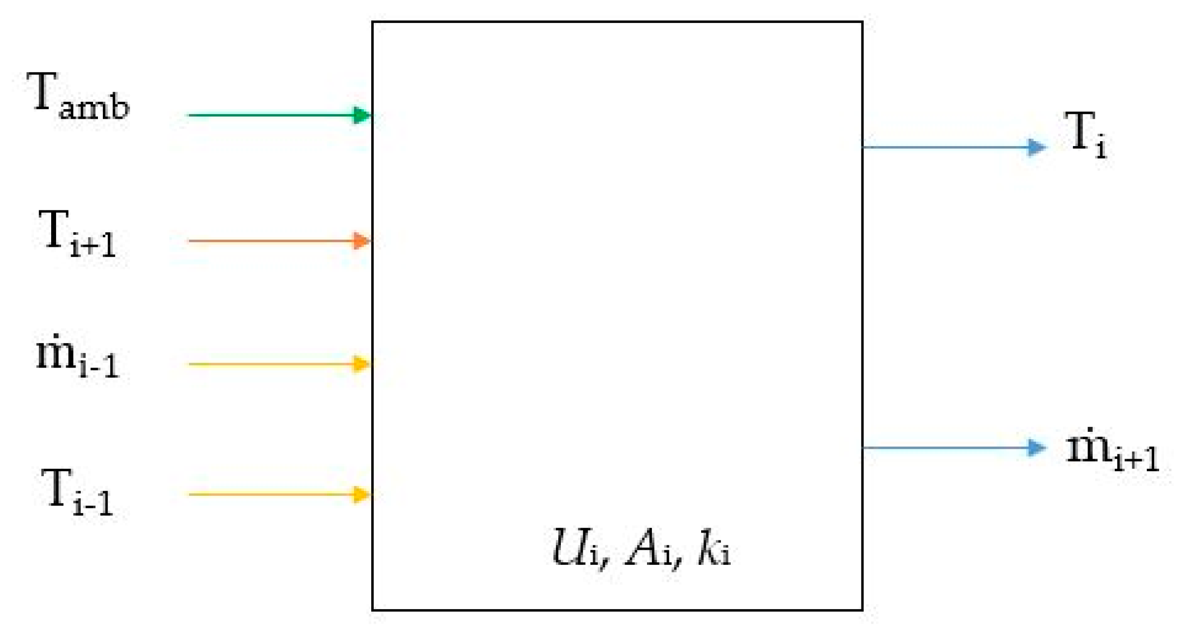
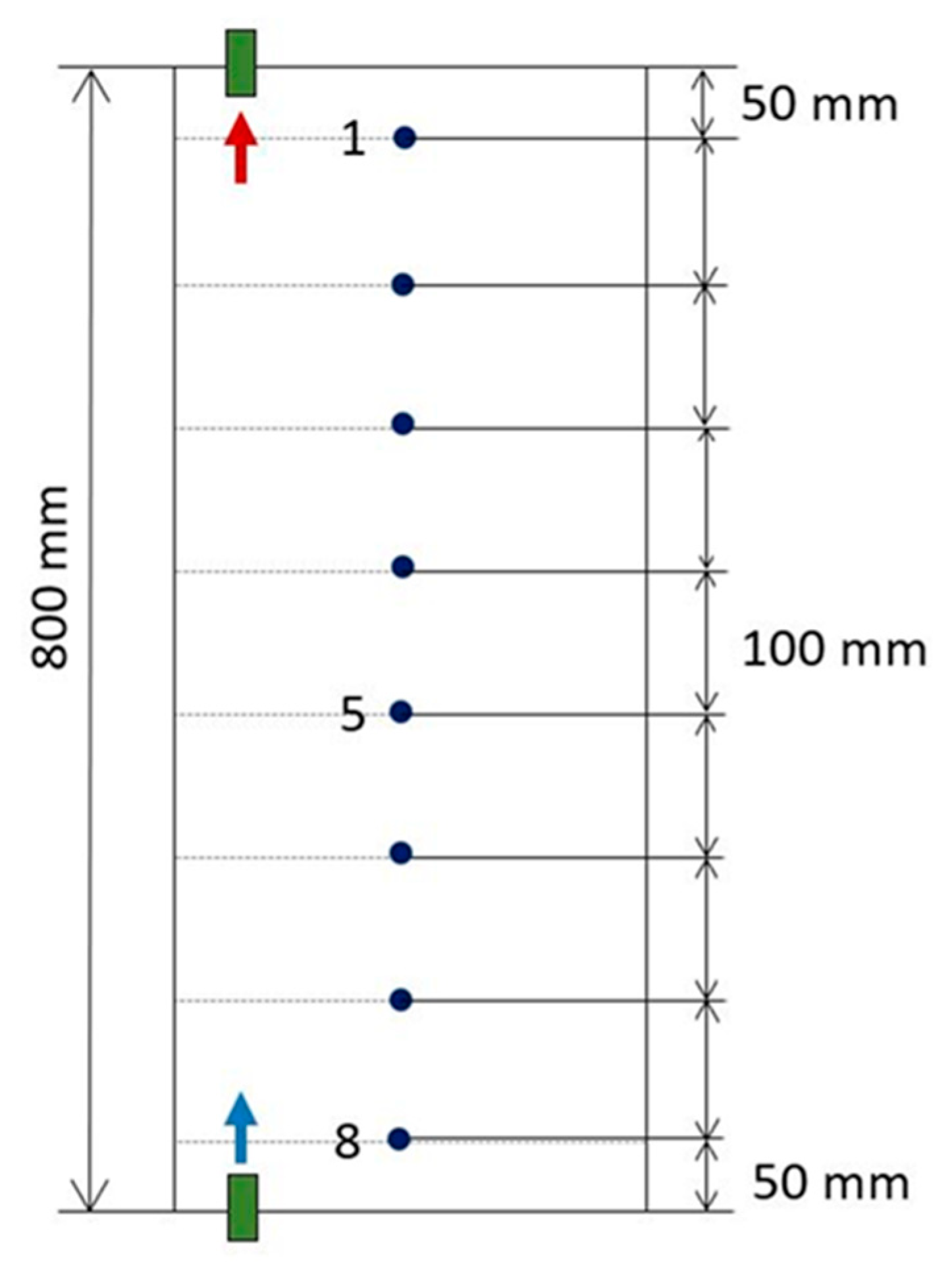
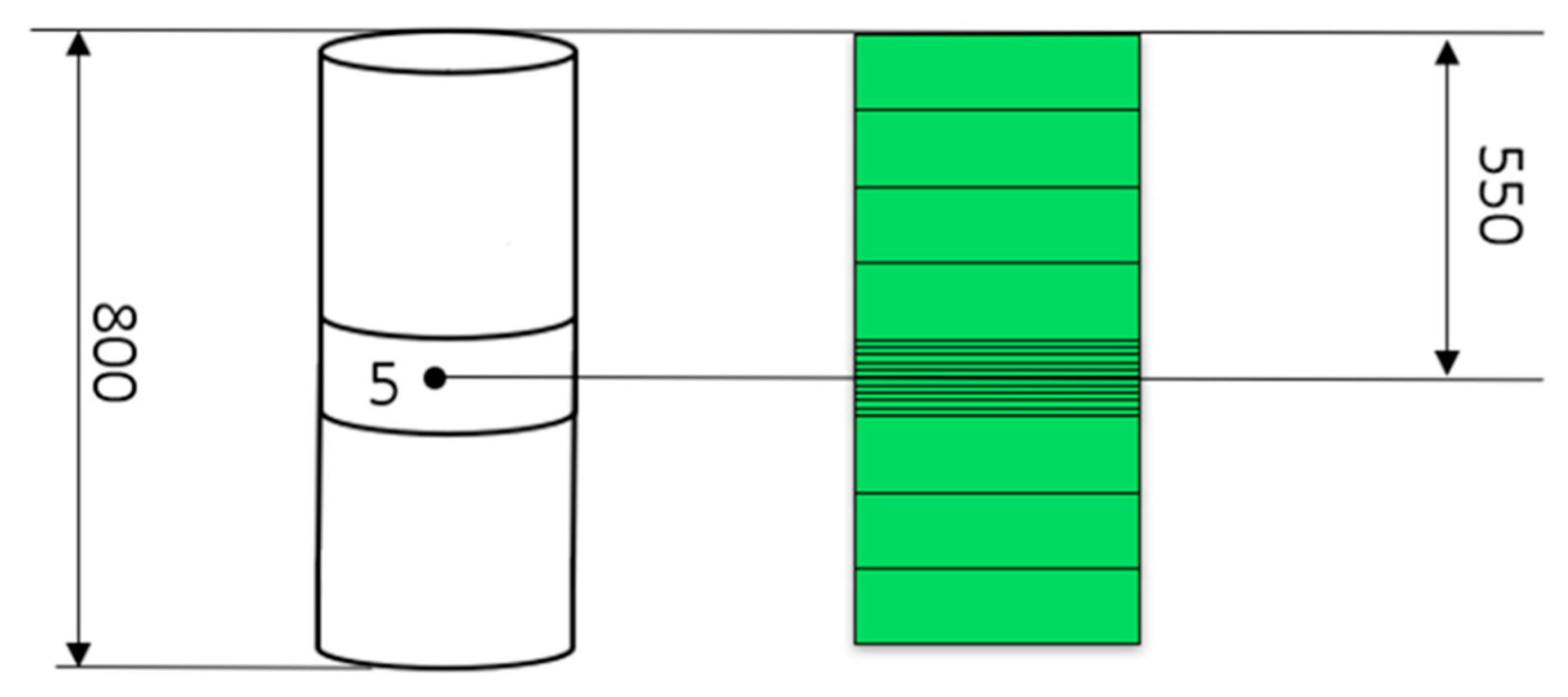
Model Implementation

The model was implemented in Matlab®/Simulink® (The MathWorks Inc., Natick, MA, USA) one of the most widely used proprietary calculation software systems, to estimate mass flow rates, temperature, and pressure in each node (respecting causal coupling with physical models of other components).
By considering the typical causality of state-determined systems, the inputs to the storage model are as follows:
  • Incoming mass flow rates and their related temperatures for each node;
  • Outgoing mass flow rates for each node but one (orange arrow in Figure 3) that is calculated by the model through the mass conservation equation.
The entry node for each incoming flow is calculated through a dedicated algorithm which, by comparing the incoming flow temperature with the temperature of the ith node, directs the flow toward the next node with the same or a higher temperature. Therefore, the storage model should consist of at least two nodes.
A mask was created which allows the user to set the general properties of the tank such as the geometrical characteristics (height, thickness, and diameter), specifications of the insulation materials, fluid properties (i.e., thermal conductivity and initial temperature), number and dimension of nodes, and convection properties.
The model is composed of two macro sections: (i) one aimed at the calculation of thermal and geometrical characteristics (i.e., overall heat loss coefficient U, area A and conduction constant k) and (ii) one intended to solve the node balance equations.
For a proper simulation, each node sub model needs several inputs, as shown in Figure 4, including the temperature of both the previous and following nodes ( T i 1 and T i + 1 ). Some parameters are derived from the model dialogue mask (Ui, Ai, ki), some are boundary terms equal for all nodes (i.e., Tamb), and others come from the previous and following nodes. The node outputs are the water temperature (Ti), the vertical mass flow rate toward the next node and where it exists, the mass flow rate which has not entered any node and is directed to the next one ( m ˙ i + 1 ). The model gives the temperature, the outgoing mass flow rate from the last node (bottom of the tank) and the outcoming pressure as the output.

3. Results

Simulations have been conducted on a single heat storage tank both in the charge and discharge phase in order to investigate the effects of overall node number on time-temperature profiles, both during charge and discharge, and the effect of the flow rates only during discharge.
The TES tank model behavior was analyzed by comparing it with the experimental data found in the literature regarding reproducible fully-instrumented laboratory tests, i.e., given by González-Altozano et al. [17] for charging and Li et al. [18] for discharging. Then the model was applied to the simulation of a large storage tank monitored in an operating environment [38].
For all the simulation sets, a variable-step ode45 (Dormand-Prince) solver was used, since it represents a good compromise between calculation time and results accuracy.

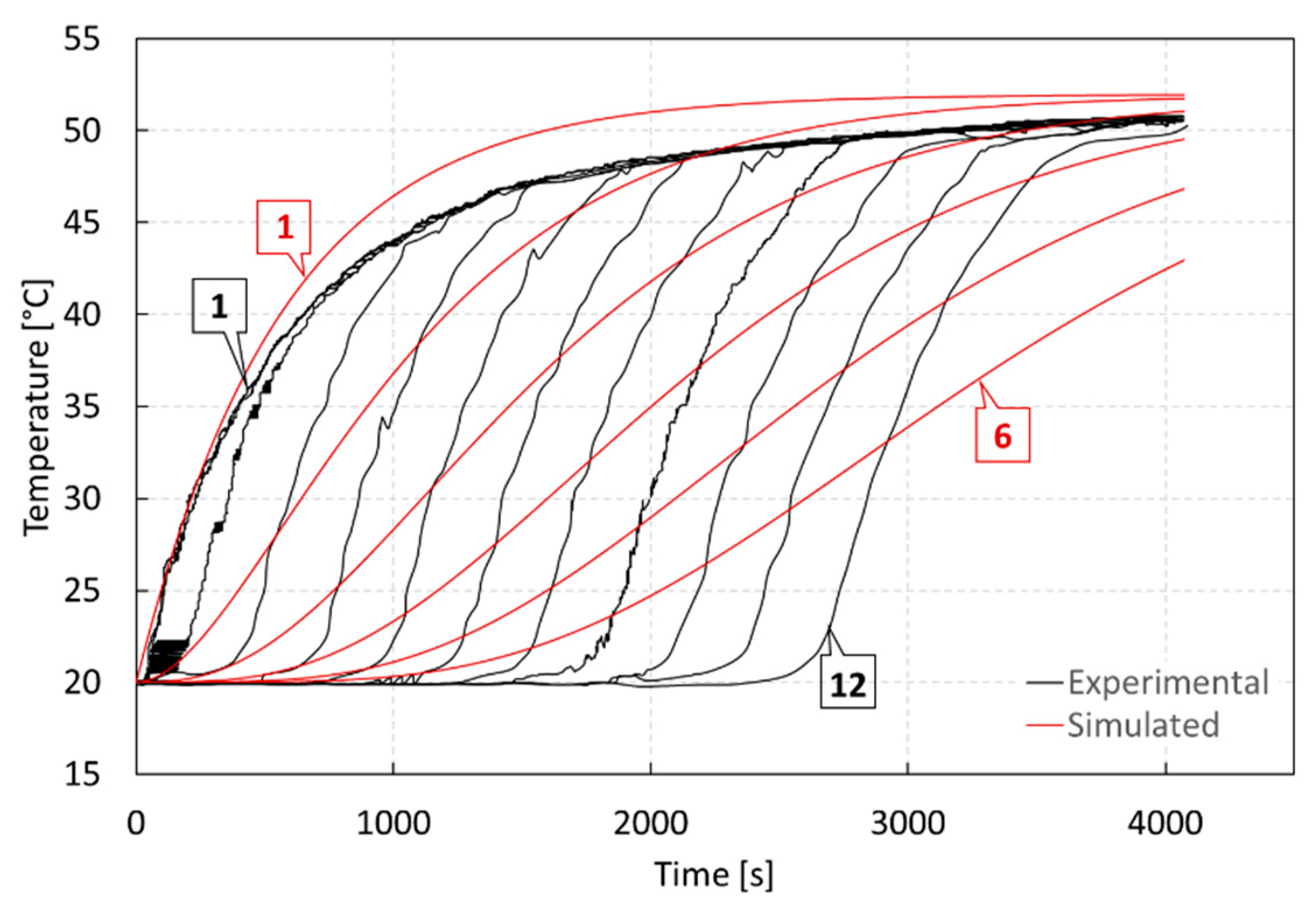
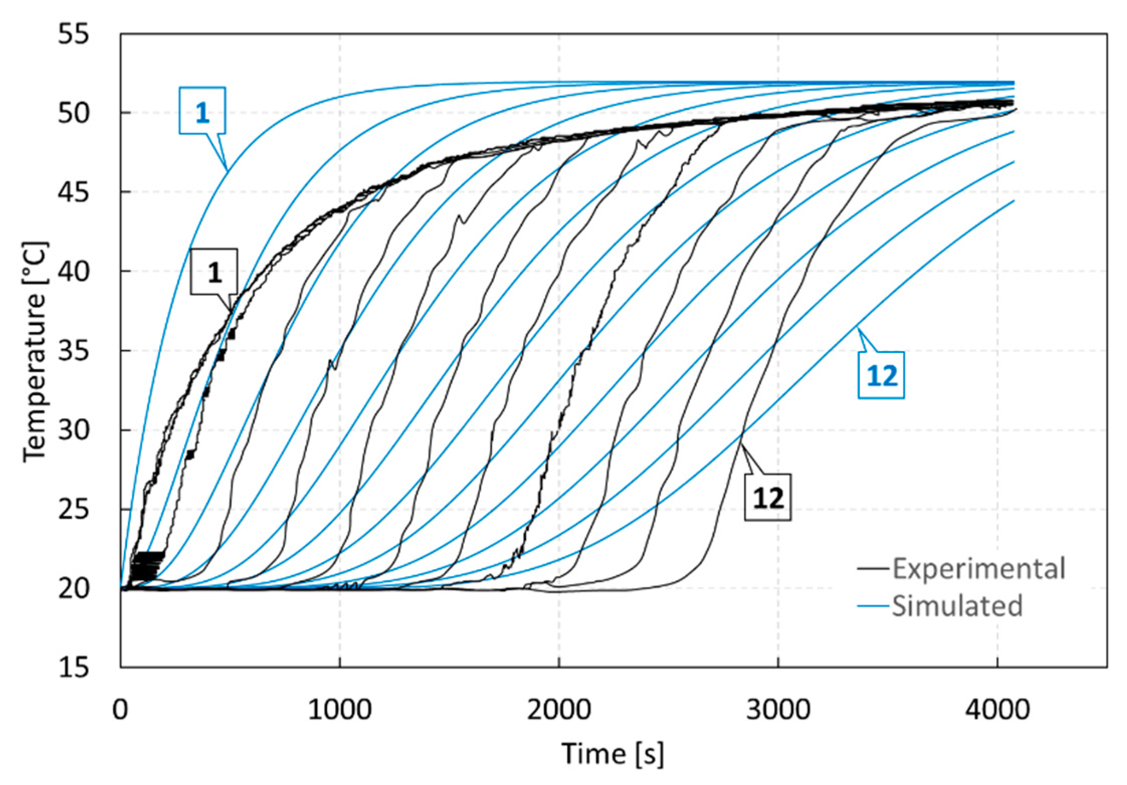
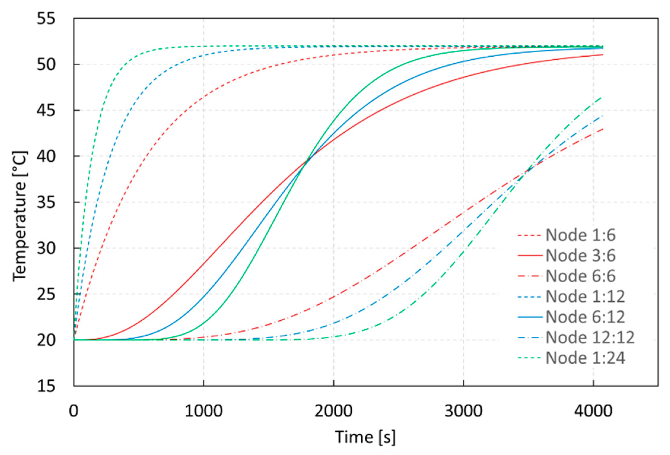
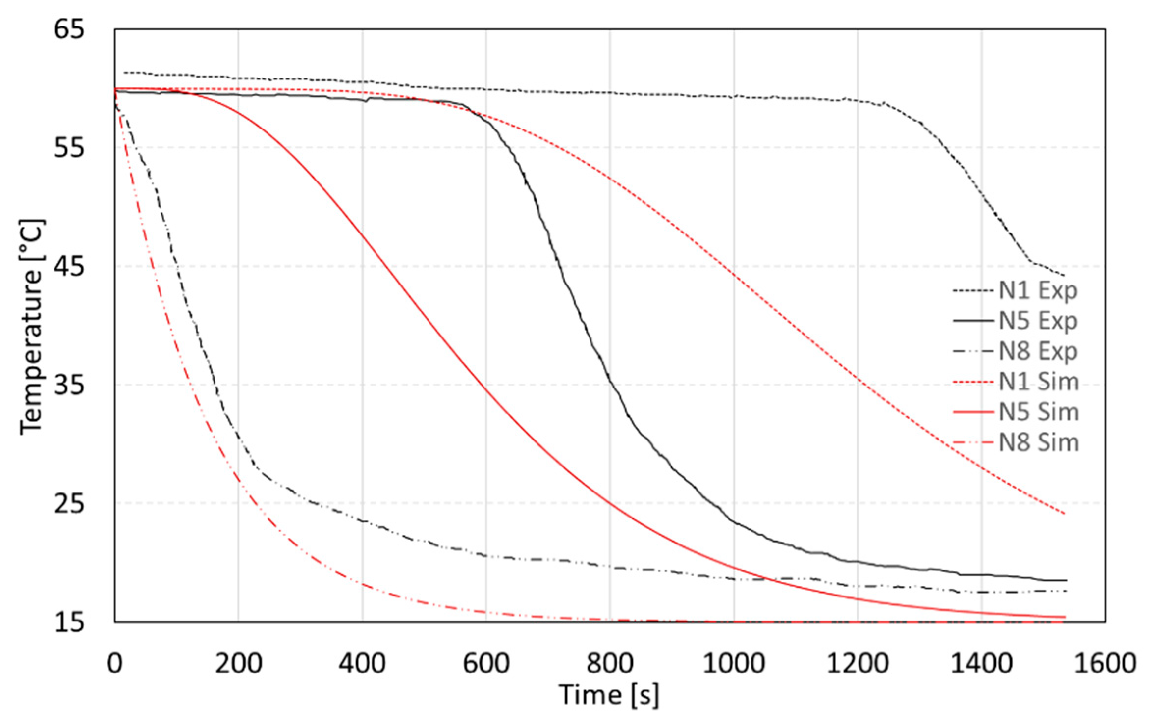
3.1. Model Analysis—Charge Phase
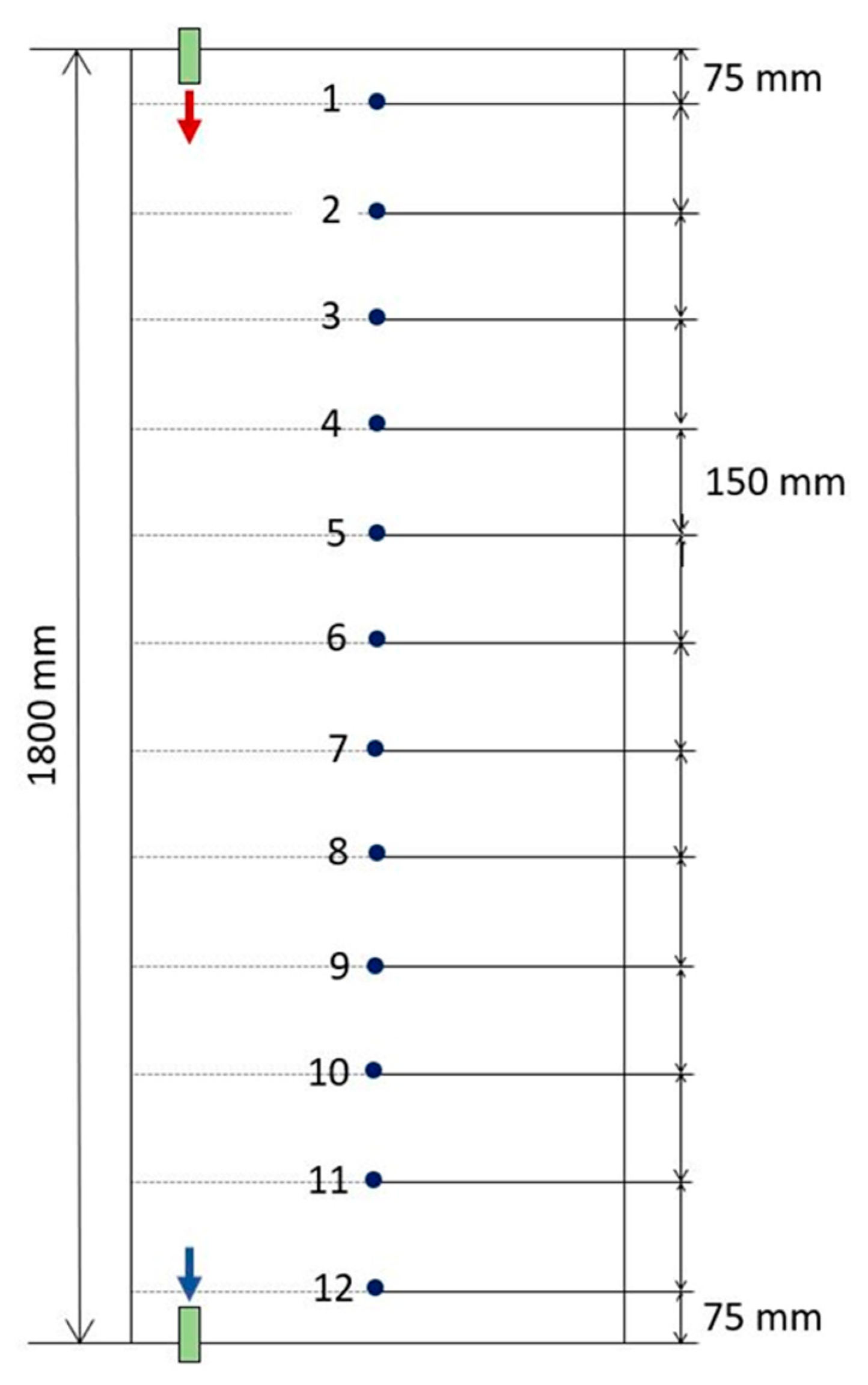
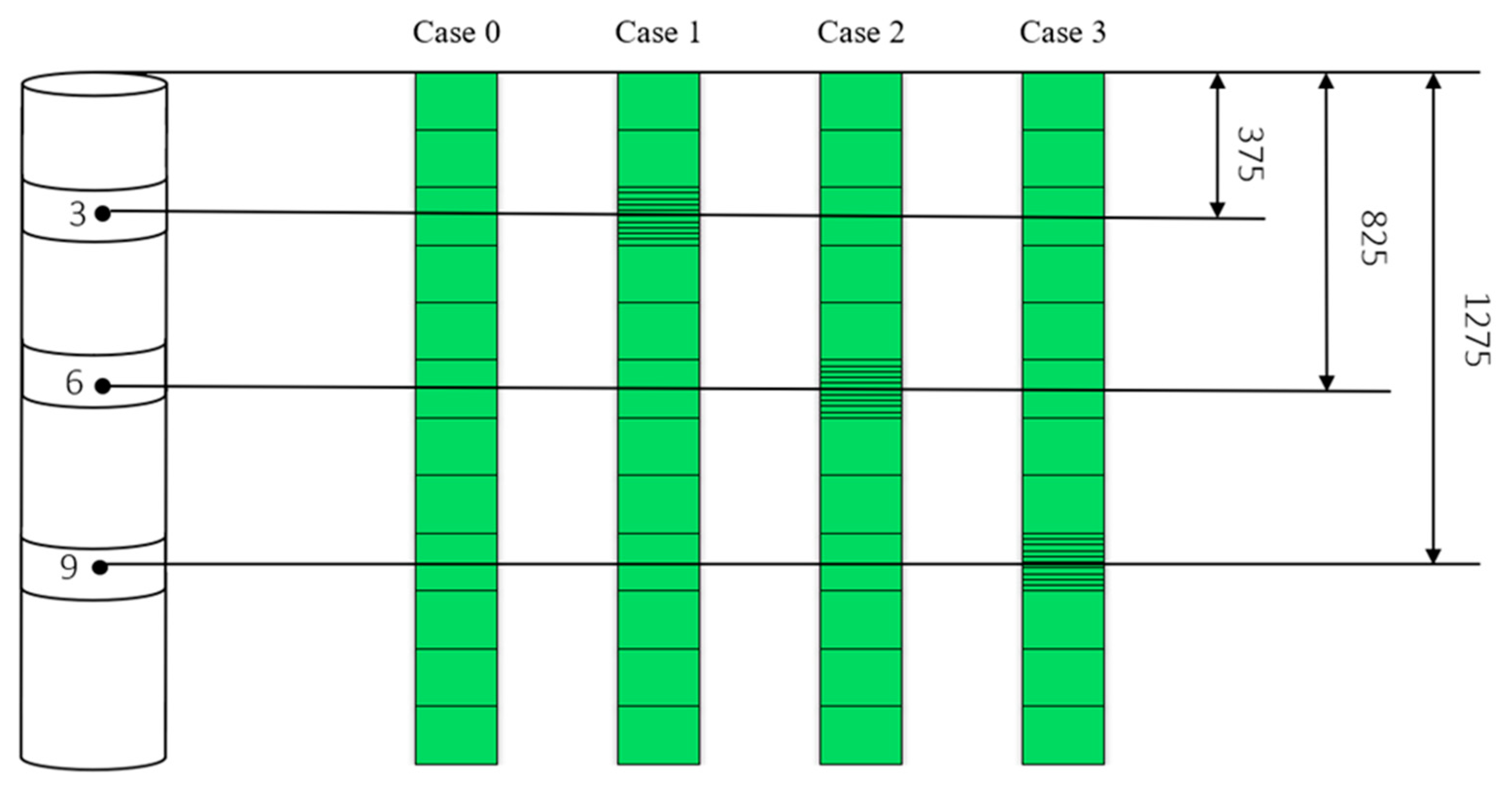
First, the charge maneuver of a thermal energy storage tank was simulated. The tank, initially at low temperature, was heated up with a hot water flow fed at the top of the tank. A grid sensitivity analysis on node number and dimension was performed.

3.1.1. Settings

According to [17], a cylindrical storage tank with a height equal to 1800 mm, an internal diameter equal to 800 mm, and a resulting volume of 0.9 m3 was considered. The side walls, the top, and the bottom of the tank were insulated with a 50-mm-thick layer of fiberglass, with thermal conductivity equal to 0.043 W/m·K. The initial temperature of the water was set to 20 °C for the whole tank and a constant volume flow rate of 16 dm3/min at 52 °C was introduced at the top of the tank, with a conventional inlet elbow. A summary of the measurement devices is given in Table 2.
González-Altozano et al. [17] placed twelve thermocouples uniformly spaced along the vertical axis of the tank, located 150 mm apart and 75 mm from both the top and the bottom of the tank, as represented in Figure 5. Therefore, N = 12 was set as the reference number for the nodes in the model.
The simulation time has been fixed at 4073 s, equal to the time declared by González-Altozano et al. [17] to replace 120% of the total storage tank volume.

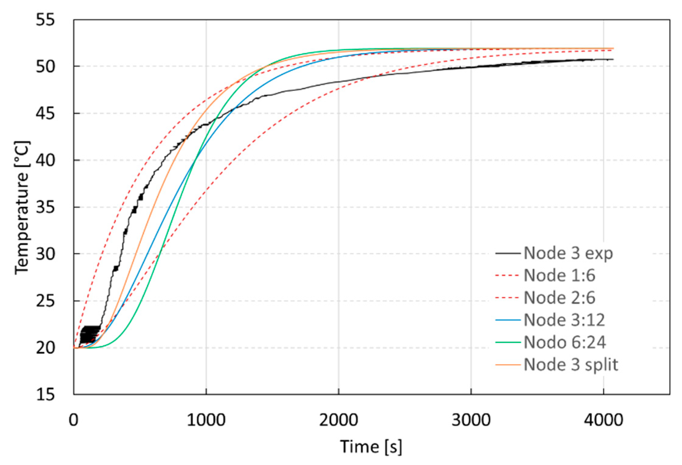
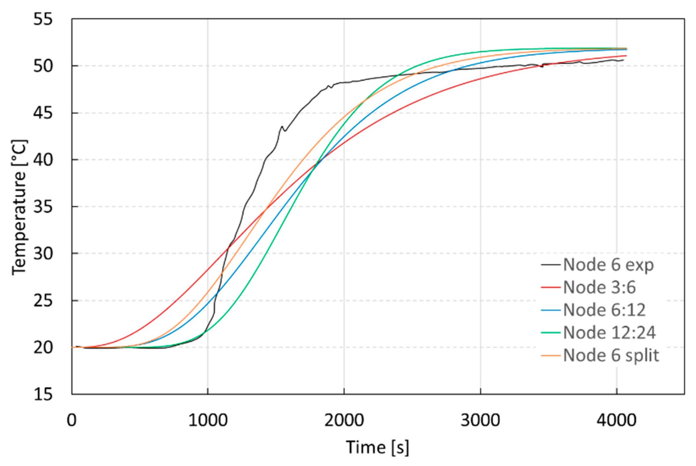
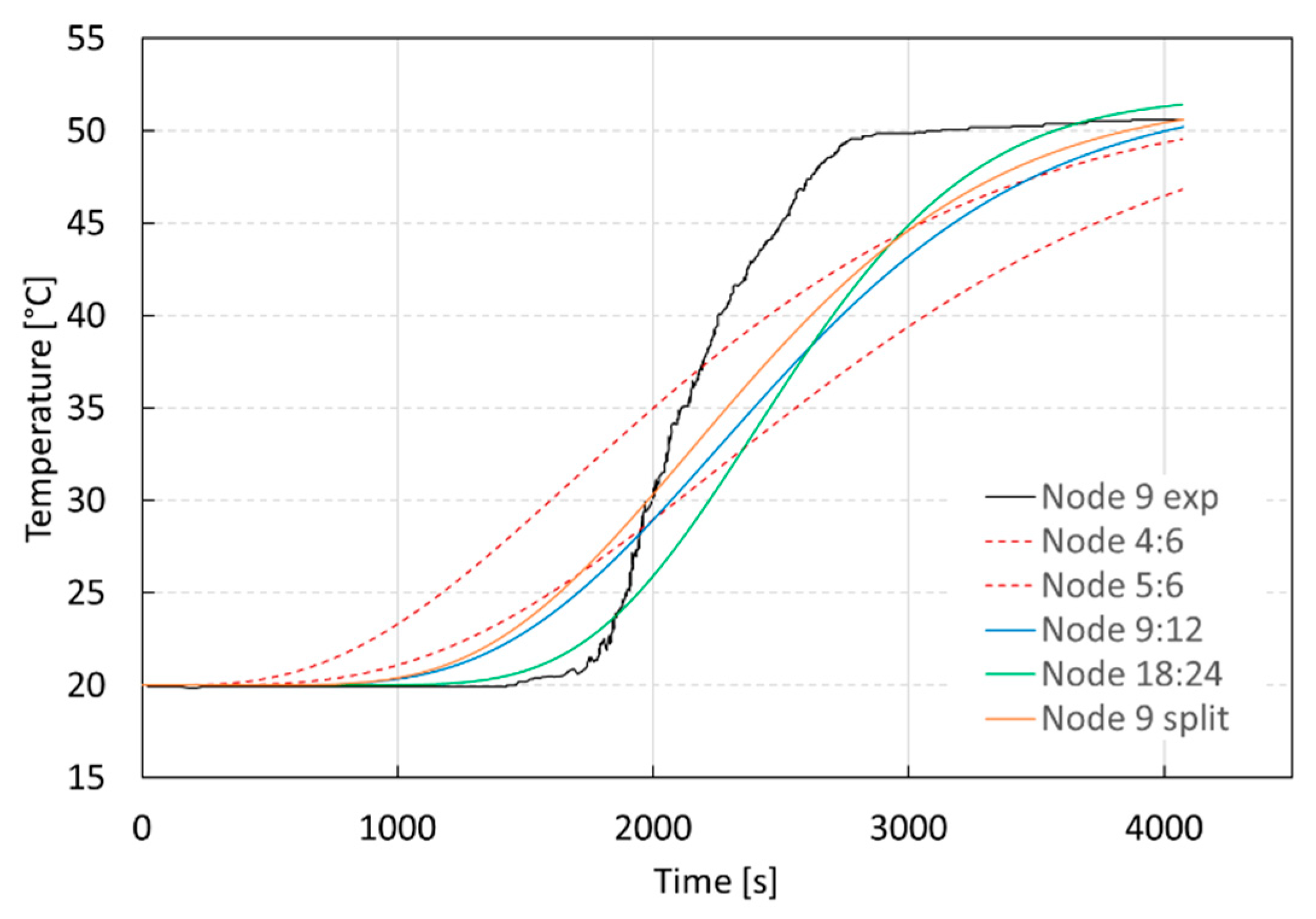
3.1.2. Sensitivity Analysis

Simulations have been conducted in three significant cases: for the reference number of nodes (N = 12), for twice the reference number of nodes (2·N) and for half the reference number of nodes (N/2). The trend of the temperature evolution against time during charging simulation for a storage tank model with 6 (Figure 6), 12 (Figure 7), and 24 nodes (Figure 8) has been recorded and compared to the experimental [17] time-temperature evolution.
As a first remark, it may be noted that simulated and experimental values of replacement time (i.e., the times required to replace the total water mass in the tank) are comparable. The results show that when the number of nodes N is increased, the thermal dynamics speeds up and the replacement time decreases toward the experimental value. Specifically, the dynamics of the upper nodes becomes faster whereas the dynamics related to the middle and the lower nodes slows down slightly in the first part—until reaching approximately 40 °C—and then increases, giving a closer match to the overall time-temperature evolution of the experiment. This latter phenomenon may be due to the thermal inertia of the upper nodes. This feature could be better appreciated in Figure 9, where for the sake of readability only the comparison of the first, middle, and last node of the three different models is shown, based on the number of nodes.
Thus, on the one hand, an increase in the number of nodes leads to faster thermal dynamics and to an improvement in accuracy of the replacement time. However, on the other hand, this highlights a specific behavior of the model. In fact, the larger the volume of a node (i.e., the lower the total node number N), the larger the mass of water inside the node and the more significant the damping effect of the incoming flow temperature. This is the case of the simulation with 6 nodes where the temperature in the first node seems to better fit the experimental temperature. This may be due to the upper zone of the storage being turbulently mixed. In fact, the temperature measured by the three thermocouples at the top are almost superimposed. On the contrary, a small number of nodes would be less beneficial when large incoming flow rates (i.e., high speed of the incoming water) are involved and there are no mixing devices—i.e., diffusers—at the inlet. In this case the incoming fluid would flow very quickly through the storage directly to the outgoing zone and without exchanging thermal energy with the crossed nodes. This operating condition cannot be described by the model because of the 1D approach used.
Thus, since the number of nodes N plays a significant role, some nodes have been split to better point out the influence that node volume plays on model accuracy. Three nodes—representative of the heights where the corresponding thermocouples are located—were chosen as reference nodes (i.e., the third, sixth, and ninth) for this purpose. Each of them was split into ten nodes, as represented in Figure 10.
The temperature evolution of each reference node after splitting was recorded and compared to those related to the experimental data and simulated results from the models with six, twelve, and twenty-four nodes (Figure 11, Figure 12 and Figure 13). The results show that by decreasing the volume of nodes and focusing the attention on a specific zone by refining the local 1D “mesh,” the calculated temperature evolution matches the measurements better and better, especially for nodes belonging to the upper part of the storage tank. This is due to the fact that the lower nodes are negatively influenced by the dynamics of the upper ones.
In conclusion, the choice of the number of nodes N determines the resolution with which the vertical temperature distribution can be modeled in the storage tank. In fact, an increase in the number of nodes will allow significant temperature gradients to be modeled more accurately (Figure 14). Thanks to versatility and accurate physical representation of stratification and heat exchanges, it seems that the model can be a useful simulation tool for the reliable prediction of temperature evolution in a stratified storage tank during charge operation.

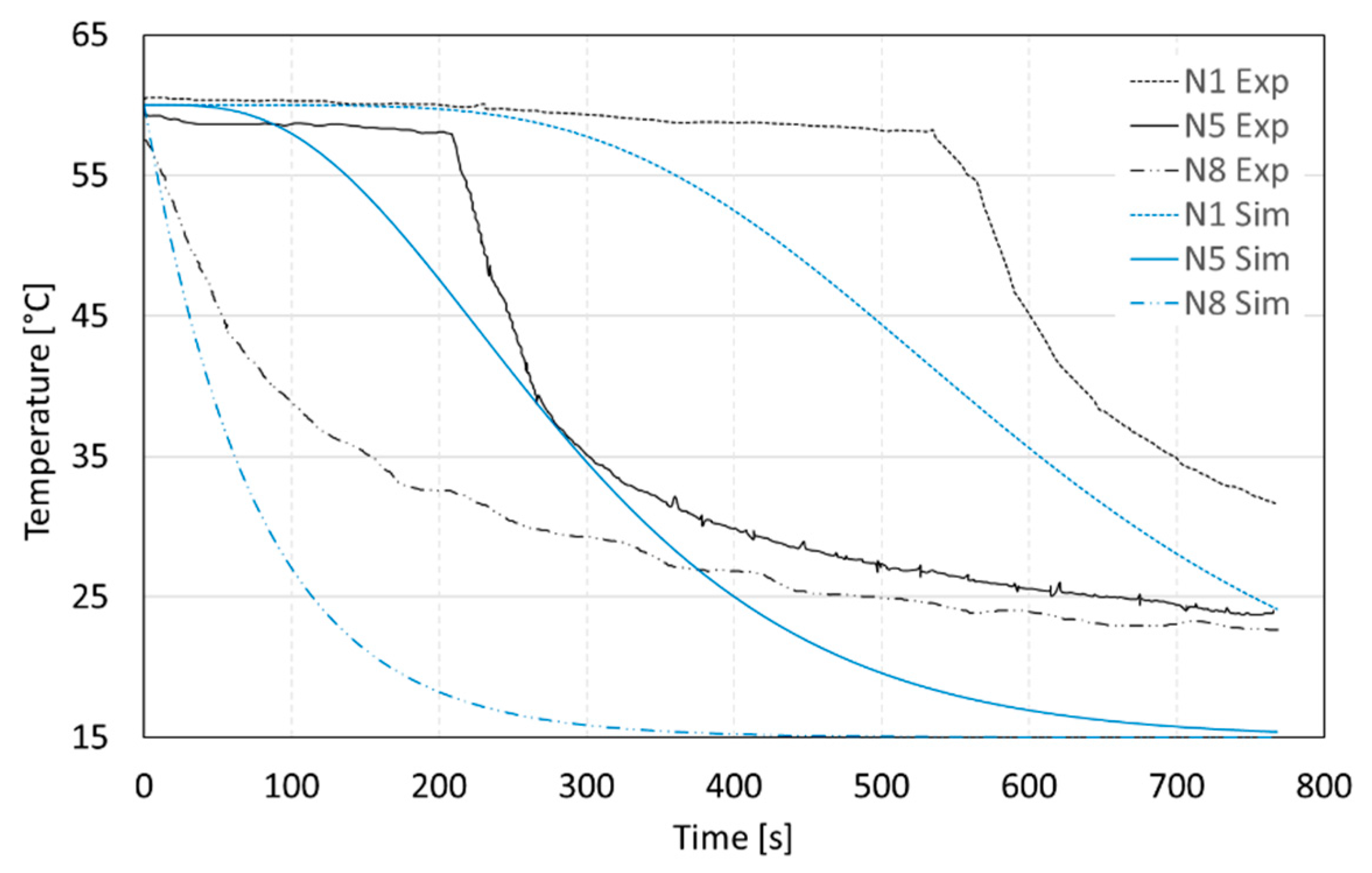
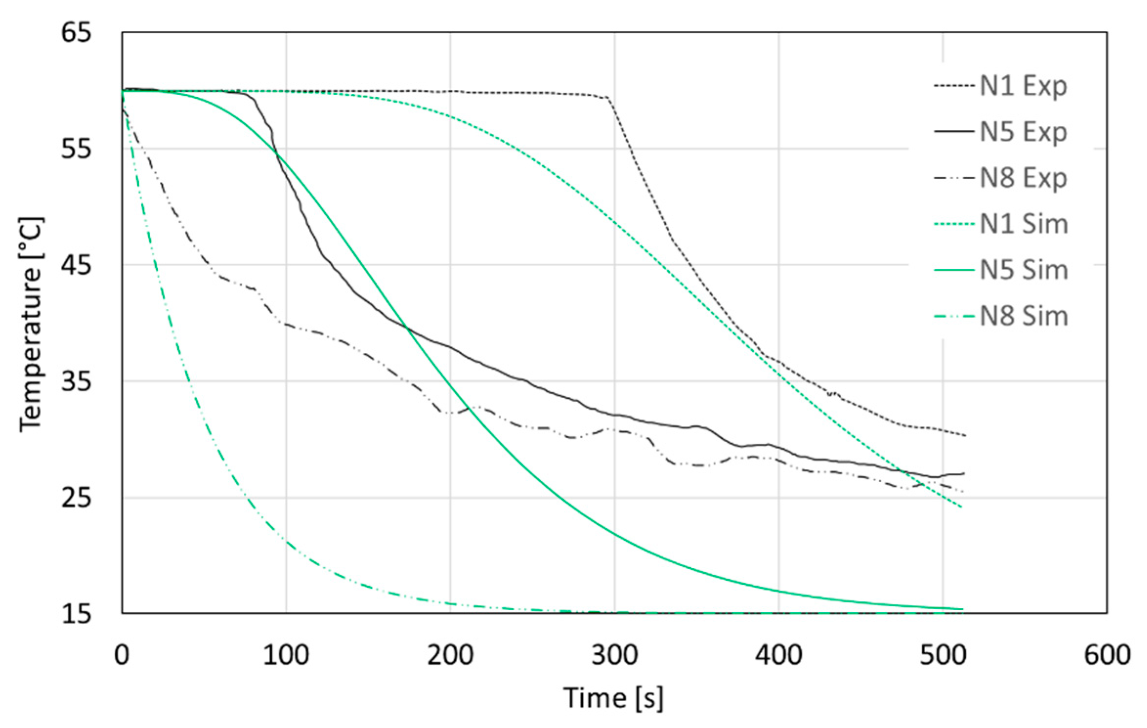
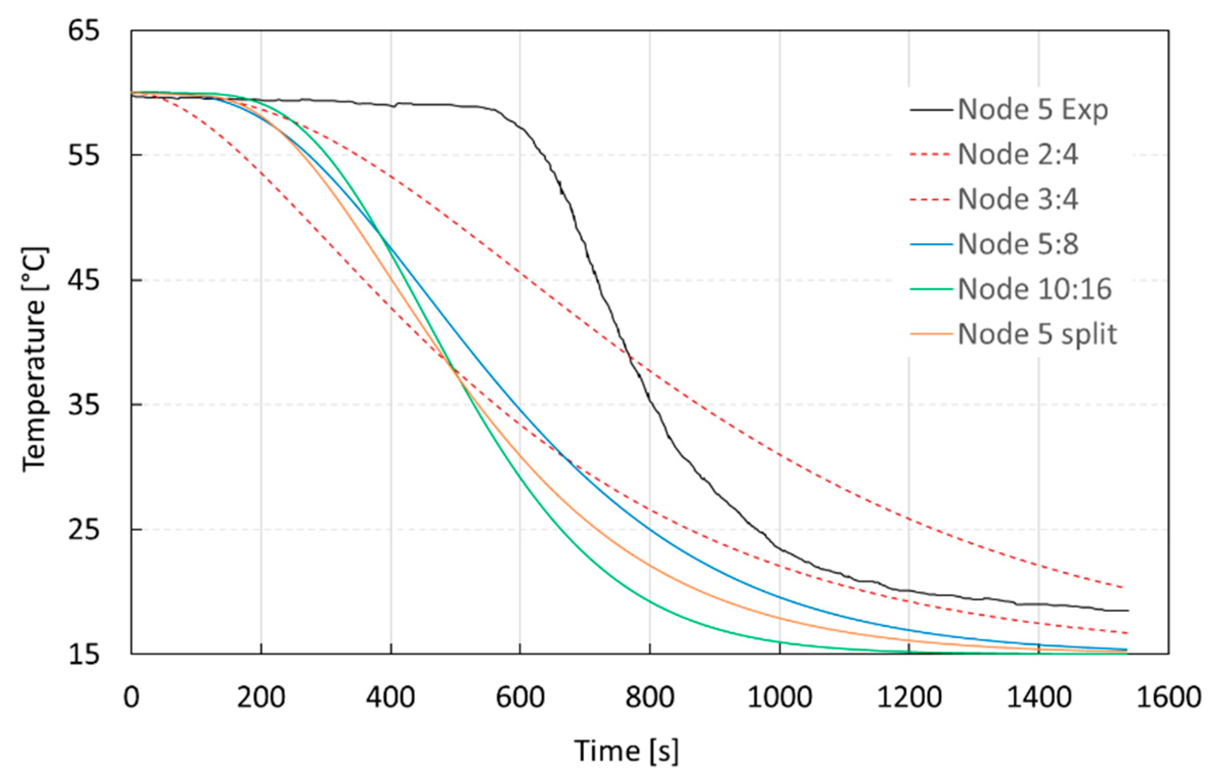
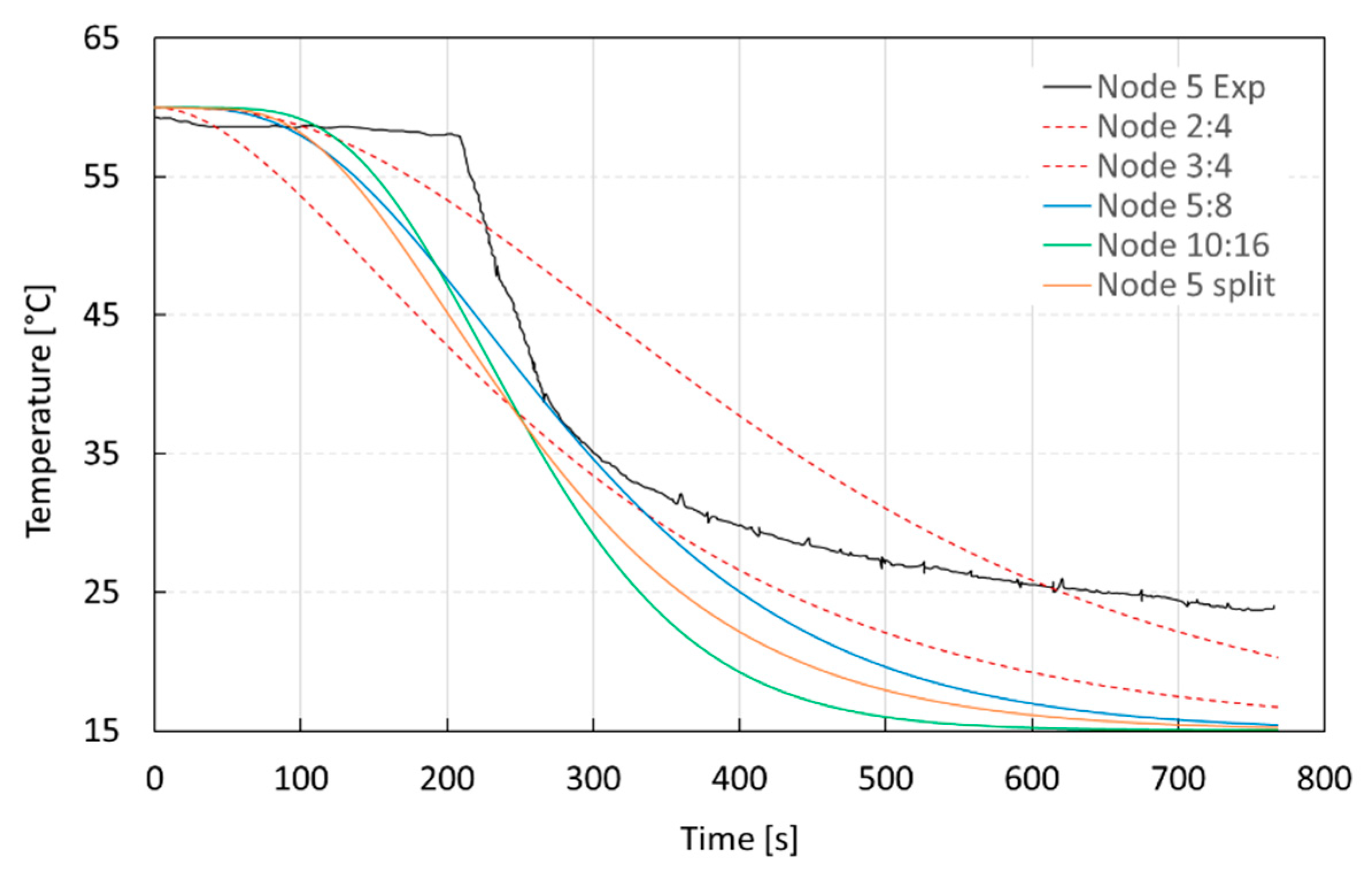
3.2. Model Analysis—Discharge Phase

Thereafter, the discharge maneuver of a thermal energy storage tank was simulated. The tank, initially at high temperature, was cooled down with the introduction of a cold-water flow. The effects of the node number and flow rate variations on temperature evolution were investigated.

3.2.1. Settings

According to [18], a cylindrical storage tank with a height of 800 mm and an internal diameter of 400 mm (resulting in a volume of 0.1 m3) was modeled. Three different flow rates (5 dm3/min, 10 dm3/min, and 15 dm3/min) at 15 °C were introduced—by means of a slotting-type inlet—at the bottom of the tank initially at 60 °C. The whole incoming flow rate exited the storage tank from the top. Li et al. [18] divided the water tank into eight layers of the same dimension fitted with one thermocouple each with a measurement time interval of 5 s. The first and the last thermocouples were located at 50 mm from the top and the bottom of the tank, respectively, whereas the intermediate ones are placed 100 mm apart (Figure 15). A summary of the measurement instrumentation is given in Table 3.
As the real tank was equipped with eight thermocouples, the model was set with a basic number of eight nodes. The simulation time was set equal to the unit replacement time, i.e., 1536 s, 768 s, and 512 s for a volume flow rate of 5 dm3/min, 10 dm3/min, and 15 dm3/min, respectively.

3.2.2. Sensitivity Analysis

Similarly to what was done for charging (Section 3.1), here again simulations were conducted in the three more significant cases: for the reference number of nodes (N = 8), for twice the reference number of nodes (2∙N) and for half the reference number of nodes (N/2). In addition, for each specific number of nodes, the three different flow rates mentioned in the settings paragraph (Section 3.2.1) were introduced alternatively.
Finally, the fifth node—representative of the height at which the fifth thermocouple is located—was chosen as the reference node and the 100 mm above and below were split into ten nodes each (Figure 16). That choice is based on the fact that the first and the last nodes—where the first and the last thermocouples are located—are not far enough from the edges of the tank to allow the corresponding node to be split.
At the beginning, the temperature evolution trend of the first, middle, and last node was plotted and compared to the experimental time-temperature evolution [18] during discharging simulation for 5 dm3/min (Figure 17), 10 dm3/min (Figure 18), and 15 dm3/min (Figure 19) volume flow rates.
Then, similarly to what has been done for charging, during discharging the calculated temperature evolution of the reference node after splitting has been plotted for the three simulations with different volume flow rates (see Section 3.2) and then compared to experimental data [18] and to the simulation with four, eight, and sixteen nodes (Figure 20, Figure 21 and Figure 22).
A first analysis shows that unit replacement times obtained from all the simulations remain comparable to the experimental results.
It can be observed that an increase in the number of nodes brings the temperature evolution closer to the experimental data, especially for small volume flow rates. It should be noted that in this case the simulated storage is small (800 mm high and 400 mm in diameter) and node splitting does significantly improve the sixteen-node model, as the node number is already limited. This feature can be better appreciated by observing the green and the orange curves in Figure 20, Figure 21 and Figure 22, which become closer and closer to each other as the incoming flow rate decreases.
To better investigate the effects of flow rate variations on temperature evolution, three different simulations were performed, each one keeping the number of nodes equal to that considered in the experimental model (N = 8).
When observing the temperature evolution of the tank for a flow rate of 5 dm3/min (Figure 17), the time temperature evolution for node #8 is comparable to the experimental data. The mismatch slightly increases as it continues toward the upper nodes. It is clear that node #1, being the furthest from the fluid inlet, has a slower response to heat exchange because it is the last one to interact with the cold inlet (then its dynamics is affected by all the other nodes with which the heat exchange takes place beforehand). That trend is reversed with an increase in the inlet flow rate (Figure 18 and Figure 19) in the sense that the higher the flow rate the better the curve representing node #1 fits the experimental data and vice versa for those representing the lower nodes (nodes #5 and #8). As a matter of fact, by observing Figure 18 and Figure 19 compared to the above-mentioned Figure 17, it can be noted that the dynamic behavior becomes faster and faster (as a greater mass of fluid exchanges heat with the water mass in the tank). The temperature at node #8 takes around 300 s for a 15 dm3/min volume flow rate, about 400 s and 800 s for a 10 dm3/min and 5 dm3/min volume flow rate, respectively, to reach the injected flow temperature (i.e., 15 °C).
Looking at the experimental curves, even after the unit replacement time (i.e., the time required to replace the whole water mass in the tank) has passed, the water temperature does not reach the temperature of the incoming flow (i.e., 15 °C). This behavior might be due to the fact that—given the experimental storage size—for high flow rates, part of the incoming fluid can be directed straight to the exit duct, and it has no time to exchange heat with the water in the tank. Thus, the water remains at a higher temperature (around 25 °C). In other words, a fraction of the inlet flow rate is bypassed, and its thermal energy is not stored in the tank.
The above-mentioned temperature behavior is not present in the results given by the simulations, as the approach followed to build up the model does not allow the flow bypass event to be considered (i.e., the entire incoming flow passes through all nodes without exchanging heat).
From these simulations it is apparent that the model results in terms of temperature changes inside the tank show deviations from the experimental data when the 3D effects become more and more significant (i.e., when the size of the tank becomes smaller and fluid velocity becomes higher). However, it should be noted that the proposed model can satisfactorily describe the physical behavior of the component within a complex energy grid, without unacceptable increases in the calculation burden.
This work points out further topics for the future development of the model. For high volume flow rates (compared to the size of the tank), the nodes furthest from the inlet section are less affected by the dynamics of the intermediate nodes. Moreover, the global heat exchange is faster, as a greater mass of fluid exchanges energy with the water in the tank.
Finally, referring to the number of nodes, it can be concluded that for small-size storage tanks the node-splitting technique does not significantly improve the accuracy of the temperature evolution inside the tank.

3.3. Model Application

In the last case study, the real daily operation of the upper region of a large atmospheric two-zone heat storage tank was investigated [38]. The aim of this last trial is to examine how the model behaves when representing the real operation of a large Thermal Energy Storage tank.

3.3.1. Settings

Unlike the previous cases, the tank in question is divided into two regions by an insulated intermediate floor. A vertical open-ended pipe serves as a hydraulic connection between the upper and the lower zone: it compensates the water density changes in the lower region and it prevents the whole tank from under-pressure or over-pressure. Furthermore, the intermediate floor—acting like an obstacle to natural convection—allows hot water in the lower zone to be stored at higher pressure if compared to an ordinary TES tank.
Since the simulation of a two-zone heat storage tank falls outside the scope of this work, only the upper region of the tank has been modeled: according to [38], it is a cylindrical tank with a height of 30 m and an internal diameter of 20 m (resulting in a volume of 9420 m3). A constant volume flow of 50 m3/h at 95 °C was introduced throughout the day by means of a radial diffuser placed at the top of the tank. The same inverse mass flow exited the storage tank from the bottom outlet. In order to evaluate the thermal stratification, the tank was equipped with a distributed temperature sensing (DTS) measurement system (resolution of about 0.1 °C) and 28 vertically aligned PT100 sensors.

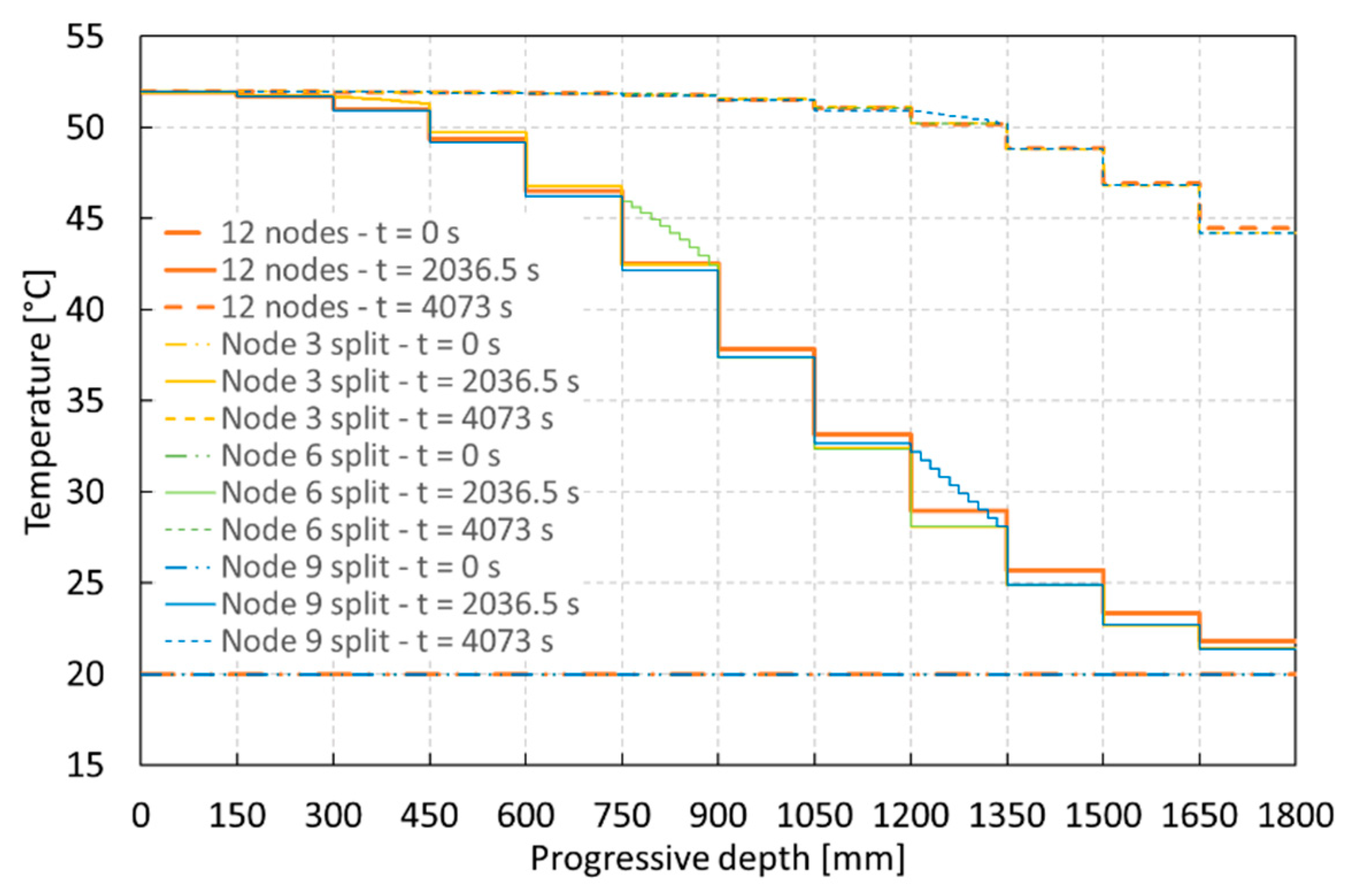
3.3.2. Simulation Results

The tank model is made up of 25 evenly spaced nodes. Initial conditions were set on the basis of the information given in [38]. For ease of comparison, the water temperature daily evolution was recorded for seven specific tank heights, at four-hour intervals. The simulation was performed by means of the Matlab® ode45 variable-step solver, which took 0.71 s to simulate the daily operation of the storage tank, with a standard laptop.
The simulation result and absolute error are shown in Table 4, together with the experimental temperatures mentioned in the reference article.
The simulated temperature profile is in good accordance with the experimental data both for the top and the bottom of the considered region; the average absolute error is equal to 1 °C. It should be observed that a slight increase in the absolute error occurs over time at the half-height of the tank region; it is probably due to the mixing of chilled water—entering the upper zone at the temperature of about 62 °C—from the compensation pipe, as reported in [38]. Since the interaction between the two zones of the storage tank is not considered in the proposed model, the simulated temperature gradients seem to be smaller than the experimental one.
Even considering this issue, the model has proved to be performant in the representation of the real operation of a large heat storage tank: the maximum absolute error does not exceed 6 °C.

4. Discussion

In this paper, a new Matlab®/Simulink® model for the simulation of stratified sensible heat storage systems was presented. The 1D model was built using the multi-node approach, solving the volume and energy balance equations for each node. Because of its innovative structure, the model is highly customizable in node number and dimension, enabling detailed investigation of the thermal stratification phenomenon.
Three experimental datasets from the literature were used as references for the model analysis and validation, by considering the charge phase, the discharge phase, and the nominal operation of heat storage tanks with different sizes.
In the case of the charge phase, the tank—initially at a low temperature—was heated up with the injection of hot-water at the top. This simulation was performed three times, by varying the number of nodes while maintaining all the other parameter values (such as tank dimension, inlet and outlet flow rates, and initial temperature of the stored water).
In the case of the discharge phase, the tank—initially at a warm temperature—was cooled down with the injection of cold-water at the bottom. In this case, both the number of nodes and the inlet flow rates were varied throughout the simulations, while maintaining the other parameter values. For a better comparison of the results, an appropriate point was chosen as reference; it corresponds to the location of the fifth thermocouple in the experimental system, it is far enough from the edges of the tank and it was matched with a specific node in every simulation.
In the real operation case, the tank was fed with hot water from the top radial diffuser. The daily temperature evolution was simulated by means of a model made up of 25 evenly spaced nodes. The simulated and experimental data were compared in order to evaluate the model performance when dealing with large storage tanks, commonly used in district heating applications.
The comparison between simulated and experimental data confirms that the choice of the number of nodes plays a significant role in the representation accuracy of thermal stratification inside the storage tank: an increase in the number of nodes—which, for a given tank capacity, corresponds to a decrease in node volume—improves the simulation results (i.e., temperature variations in the tank) allowing more accurate temperature gradients.
The model proposed in this paper proved to be able to give an accurate physical representation of stratification and heat exchange phenomena in sensible heat storage systems and can be a useful tool to reliably simulate temperature changes in stratified storage tanks. Its innovative features are flexibility and adaptability, which make it possible to choose the number and dimensions of each node in the model, allowing the user to focus the simulation on a specific zone of interest.
However, the model shows limitations for some specific storage configurations. If the ratio between the inlet flow rate and the node volume is too small, the thermal stratification dynamics slows down and the simulation becomes inaccurate; the larger the node volume, the greater the mass of water contained and the higher the mixing effect that dampens the incoming flow temperature. Furthermore, the simplified representation of convection can lead to discrepancies between the real and the simulated temperature evolutions, as is the case for the models reported in the literature. Another limitation was detected in small storage tank simulations; for high flow rates and large temperature differences between the incoming and the stored fluid, a fraction of the incoming fluid may flow directly to the exit duct without exchanging heat with the stored water. In other words, part of the fluid is bypassed, and its thermal energy is not stored. The developed model is not able to reproduce this phenomenon as—due to the 1D approach followed—all the incoming flows pass through all the nodes.
It should be recalled that the stratified storage model was developed to become part of a library of physics-based components for the dynamic simulation of district heating networks. In these applications the involved storage tanks are large and the temperature differences between the incoming and stored water temperature are usually fairly low, and therefore the above-mentioned drawbacks of the proposed 1D model are acceptable, compared to the advantage of keeping low calculation times.

Author Contributions

Conceptualization, A.G., M.M. and M.R.; funding acquisition and supervision, A.G. and M.M.; investigation, validation and writing, N.C. and A.D.L.

Funding

This work was supported by the “Efficity—Efficient Energy Systems for Smart Urban Districts” project (CUP E38I16000130007) co-funded by the Emilia-Romagna Region through the European Regional Development fund 2014–2020.

Conflicts of Interest

The authors declare no conflict of interest.

Nomenclature

Am2area
EJenergy
MKgmass
Q ˙ Wheat flow
T°Ctemperature
UW/(m2·K)overall heat exchange coefficient
V ˙ m3/svolume flow
cJ/(kg·K)specific heat
hJ/(kg·K)specific enthalpy
kW/Kconduction constant
m ˙ kg/smass flow rate
tstime

Subscripts and Superscripts

amb.ambient
iindex
inincoming
outoutgoing
vertvertical

References

  1. Sharma, A.; Tyagi, V.V.; Chen, C.R.; Buddhi, D. Review on thermal energy storage with phase change materials and applications. Renew. Sustain. Energy Rev. 2009, 13, 318–345. [Google Scholar] [CrossRef]
  2. Nkwetta, D.N.; Haghighat, F. Thermal energy storage with phase change material—A state-of-the art review. Sustain. Cities Soc. 2014, 10, 87–100. [Google Scholar] [CrossRef]
  3. Barbieri, E.S.; Melino, F.; Morini, M. Influence of the thermal energy storage on the profitability of micro-CHP systems for residential building applications. Appl. Energy 2012, 97, 714–722. [Google Scholar] [CrossRef]
  4. Ibrahim, H.; Ilinca, A.; Perron, J. Energy storage systems-Characteristics and comparisons. Renew. Sustain. Energy Rev. 2008, 12, 1221–1250. [Google Scholar] [CrossRef]
  5. Dincer, I.; Rosen, M.A. Thermal Energy Storage: Systems and Applications, 2nd ed.; John Wiley & Sons: Oshawa, ON, Canada, 2011. [Google Scholar]
  6. Gambarotta, A.; Morini, M.; Rossi, M.; Stonfer, M. A Library for the Simulation of Smart Energy Systems: The Case of the Campus of the University of Parma. Energy Procedia 2017, 105, 1776–1781. [Google Scholar] [CrossRef]
  7. Cadau, N.; De Lorenzi, A.; Gambarotta, A.; Morini, M.; Saletti, C. A Model-in-the-Loop application of a Predictive Controller to a District Heating system. Energy Procedia 2018, 148, 352–359. [Google Scholar] [CrossRef]
  8. Dainese, C.; Faè, M.; Gambarotta, A.; Morini, M.; Premoli, M.; Randazzo, G.; Rossi, M.; Rovati, M.; Saletti, C. Development and application of a Predictive Controller to a mini district heating network fed by a biomass boiler. Energy Procedia 2019, 159, 48–53. [Google Scholar] [CrossRef]
  9. Gambarotta, A.; Morini, M.; Saletti, C. Development of a Model-based Predictive Controller for a heat distribution network. Energy Procedia 2018, 2896–2901. [Google Scholar] [CrossRef]
  10. Kalaiselvam, S.; Parameshwaran, R. Thermal Energy Storage Technologies for Sustainability, 1st ed.; Academic Press: Cambridge, MA, USA, 2014. [Google Scholar]
  11. Ould Amrouche, S.; Rekioua, D.; Rekioua, T.; Bacha, S. Overview of energy storage in renewable energy systems. Int. J. Hydrog. Energy 2016, 41, 20914–20927. [Google Scholar] [CrossRef]
  12. Sarbu, I.; Sebarchievici, C. A Comprehensive Review of Thermal Energy Storage. Sustainability 2018, 10, 191. [Google Scholar] [CrossRef]
  13. Noro, M.; Lazzarin, R.M.; Busato, F. Solar cooling and heating plants: An energy and economic analysis of liquid sensible vs phase change material (PCM) heat storage. Int. J. Refrig. 2014, 39, 104–116. [Google Scholar] [CrossRef]
  14. Alva, G.; Lin, Y.; Fang, G. An overview of thermal energy storage systems. Energy 2018, 144, 341–378. [Google Scholar] [CrossRef]
  15. Drück, H.; Pauschinger, T. Multiport Store—Model for TRNSYS—Type 340; Institut für Thermodynamik und Wärmetechnik (ITW) Universität Stuttgart: Stuttgart, Germany, 2006. [Google Scholar]
  16. Wemhöner, C.; Hafner, B.; Schwarzer, K. Simulation of Solar Thermal Systems with Carnot Blockset in the Environment Matlab® Simulink®. In Proceedings of the Eurosun Conference 2000, Copenhagen, Denmark, 19–23 June 2000. [Google Scholar]
  17. González-Altozano, P.; Gasque, M.; Ibáñez, F.; Gutiérrez-Colomer, R.P. New methodology for the characterisation of thermal performance in a hot water storage tank during charging. Appl. Therm. Eng. 2015, 84, 196–205. [Google Scholar] [CrossRef]
  18. Li, S.H.; Zhang, Y.X.; Li, Y.; Zhang, X.S. Experimental study of inlet structure on the discharging performance of a solar water storage tank. Energy Build. 2014, 70, 490–496. [Google Scholar] [CrossRef]
  19. Njoku, H.O.; Ekechukwu, O.V.; Onyegegbu, S.O. Analysis of stratified thermal storage systems: An overview. Heat Mass Transf. 2014, 50, 1017–1030. [Google Scholar] [CrossRef]
  20. Dumont, O.; Carmo, C.; Dickes, R.; Georges, E.; Quoilin, S.; Lemort, V. Hot water tanks: How to select the optimal modelling approach? In Proceedings of the 12th REHVA World Congress, Aalborg, Denmark, 22–25 May 2016. [Google Scholar]
  21. Yoo, H.; Kim, C.J.; Kim, C.W. Approximate analytical solutions for stratified thermal storage under variable inlet temperature. Sol. Energy 1999, 66, 47–56. [Google Scholar] [CrossRef]
  22. Yoo, H.; Pak, E.T. Analytical solutions to a one-dimensional finite-domain model for stratified thermal storage tanks. Sol. Energy 1996, 56, 315–322. [Google Scholar] [CrossRef]
  23. Campos Celador, A.; Odriozola, M.; Sala, J.M. Implications of the modelling of stratified hot water storage tanks in the simulation of CHP plants. Energy Convers. Manag. 2011, 52, 3018–3026. [Google Scholar] [CrossRef]
  24. Dickes, R.; Desideri, A.; Lemort, V.; Quoilin, S. Model reduction for simulating the dynamic behavior of parabolic troughs and a thermocline energy storage in a micro-solar power unit. In Proceedings of the ECOS Conference 2015, Pau, France, 29 June–3 July 2015. [Google Scholar]
  25. Chung, J.D.; Shin, Y. Integral approximate solution for the charging process in stratified thermal storage tanks. Sol. Energy 2011, 85, 3010–3016. [Google Scholar] [CrossRef]
  26. Duffie, J.A.; Beckman, W.A. Solar Engineering of Thermal Processes, 4th ed.; John Wiley & Sons: Oshawa, ON, Canada, 2013. [Google Scholar]
  27. Nash, A.; Jain, N. Dynamic Modeling and Performance Analysis of Sensible Thermal Energy Storage Systems. In Proceedings of the 4th International High-Performance Buildings Conference, Purdue, Indiana, 11–14 July 2016. [Google Scholar]
  28. Chacker, A.; Bouchetiba, H. Thermal behaviour of a storage tank of solar water heater in cases of charge and discharge. Int’l J. Comput. Commun. Instrum. Engg 2017, 4, 73–77. [Google Scholar] [CrossRef]
  29. Franke, R. Object-oriented modeling of solar heating systems. Sol. Energy 1997, 60, 171–180. [Google Scholar] [CrossRef]
  30. De Césaro Oliveski, R.; Krenzinger, A.; Vielmo, H.A. Comparison between models for the simulation of hot water storage tanks. Sol. Energy 2003, 75, 121–134. [Google Scholar] [CrossRef]
  31. Bouhal, T.; Fertahi, S.; Agrouaz, Y.; El Rhafiki, T.; Kousksou, T.; Jamil, A. Numerical modeling and optimization of thermal stratification in solar hot water storage tanks for domestic applications: CFD study. Sol. Energy 2017, 157, 441–455. [Google Scholar] [CrossRef]
  32. Cabelli, A. Storage tanks—A numerical experiment. Sol. Energy 1977, 19, 45–54. [Google Scholar] [CrossRef]
  33. Badescu, V. Optimal operation of thermal energy storage units based on stratified and fully mixed water tanks. Appl. Therm. Eng. 2004, 24, 2101–2116. [Google Scholar] [CrossRef]
  34. Aisa, A.; Iqbal, T. Modelling and simulation of a solar water heating system with thermal storage. In Proceedings of the 7th IEEE Annual Information Technology, Electronics and Mobile Communication Conference, Vancouver, BC, Canada, 13–15 October 2016. [Google Scholar] [CrossRef]
  35. Cruickshank, C. Evaluation of a Stratified Multi-Tank Thermal Storage for Solar Heating Applications. Ph.D. Thesis, Queen’s University, Kingston, ON, Canada, June 2009. [Google Scholar]
  36. van Koppen, C.W.J.; Thomas, P.S.; Veltkamp, W.B. Actual benefits of thermally stratified storage in a small and a medium size solar system. In Proceedings of the International Solar Energy Society Silver Jubilee Congress, Atlanta, GA, USA, 28 May–1 June 1979. [Google Scholar]
  37. Furbo, S.; Mikkelsen, S.E. Is low flow operation an advantage for solar heating systems? In Proceedings of the Biennial Congress of the International Solar Energy Society, Hamburg, Germany, 13–18 September 1987; pp. 962–966. [Google Scholar] [CrossRef]
  38. Herwig, A.; Umbreit, L.; Rühling, K. Measurement-based modelling of large atmospheric heat storage tanks. In Proceedings of the 16th International Symposium on District Heating and Cooling, Hamburg, Germany, 9–12 September 2018. [Google Scholar] [CrossRef]
Figure 1. Liquid storage tank schematic representation for the multi-node modeling approach.
Energies 12 04275 g001
Figure 2. Generic node schematic representation.
Energies 12 04275 g002
Figure 3. Schematic representation of nodal approach for stratified storage tank, showing incoming, outgoing, and vertical mass flows.
Energies 12 04275 g003
Figure 4. Main input and output parameters for ith node.
Energies 12 04275 g004
Figure 5. Schematic representation of the experimental tank for the charge phase [9]. The hot water inlet (red arrow) and the cold-water outlet (blue arrow) are placed at the top and the bottom of the tank, respectively.
Energies 12 04275 g005
Figure 6. Temperature evolution during the charge phase—experimental vs. simulated (6 nodes).
Energies 12 04275 g006
Figure 7. Temperature evolution during the charge phase—experimental vs. simulated (12 nodes).
Energies 12 04275 g007
Figure 8. Temperature evolution during the charge phase—experimental vs. simulated (24 nodes).
Energies 12 04275 g008
Figure 9. Temperature evolution during the charge phase from models with a different number of nodes.
Energies 12 04275 g009
Figure 10. Reference node splitting for the investigation of the influence that node volume plays on model accuracy (heights in millimeters).
Energies 12 04275 g010
Figure 11. Experimental temperature evolution during the charge phase at node #3 vs. simulation results.
Energies 12 04275 g011
Figure 12. Experimental temperature evolution during the charge phase at node #6 vs. simulation results.
Energies 12 04275 g012
Figure 13. Experimental temperature evolution during the charge phase at node #9 vs. simulation results.
Energies 12 04275 g013
Figure 14. Temperature stratification (during the charge phase) inside the storage tank at three different simulation stages.
Energies 12 04275 g014
Figure 15. Schematic representation of the experimental tank for the discharge phase [10]. The cold-water inlet (blue arrow) and the hot water outlet (red arrow) are placed at the bottom and the top of the tank, respectively.
Energies 12 04275 g015
Figure 16. Reference node (#5) splitting for the investigation of the influence that node volume plays on model accuracy (heights in millimeters).
Energies 12 04275 g016
Figure 17. Temperature evolution during the discharge phase—experimental vs. simulated—5 dm3/min volume flow rate.
Energies 12 04275 g017
Figure 18. Temperature evolution during the discharge phase—experimental vs. simulated—10 dm3/min volume flow rate.
Energies 12 04275 g018
Figure 19. Temperature evolution during the discharge phase—experimental vs. simulated—15 dm3/min volume flow rate.
Energies 12 04275 g019
Figure 20. Experimental temperature evolution at node #5 vs. simulation results—5 dm3/min volume flow rate—discharge phase.
Energies 12 04275 g020
Figure 21. Experimental temperature evolution at node #5 vs. simulation results—10 dm3/min volume flow rate—discharge phase.
Energies 12 04275 g021
Figure 22. Experimental temperature evolution at node #5 vs. simulation results—15 dm3/min volume flow rate—discharge phase.
Energies 12 04275 g022
Table 1. Pros and cons for each thermal energy storage (TES) tank modeling approach.
Model DimensionProsCons
0D
🗸
Straightforward implementation
🗸
Low simulation time (lower than Real Time)
🗶
Accurate only for small volume storage tanks
🗶
Complex phenomena (e.g., convection and conduction) cannot be considered
1D
🗸
Modest implementation effort
🗸
Model simplicity
🗸
Limited simulation time (close to Real Time)
🗸
Reduced number of model equations
🗶
Limited accuracy for high flow rates and complex geometries
🗶
Not able to describe flow pattern in detail especially during fast-changing operating conditions
2D-3D
🗸
More detailed description of flow pattern in storage volume
🗸
Required for detailed storage system design
🗶
Difficult implementation
🗶
Large number of model equations
🗶
High simulation times
🗶
High CPU power
Table 2. Measurement devices used for the charge experimental trial.
QuantityInstrumentTask
12Thermocouples (Type T—Class 1)
(error < ±0.2%)
Measure the water temperature in the tank
2Thermocouples (Type T—Class 1)
(error < ±0.2%)
Measure the water inlet and outlet temperature during the charge process
1Electromagnetic flowmeter
Endress Hauser—mod. 53H08 DN8
(error < ± 0.1%)
Measure the water inlet mass flow rate
1Data acquisition system
National Instruments—mod. DAQ 9178
Collect sensor data
1Thermocouples input module
National Instruments—mod. 9213
TC signal conditioning and acquisition
1Flowmeter input module
National Instruments—mod. 9208
Flow-meter signal acquisition
Table 3. Measurement devices used for the discharge experimental trial.
QuantityInstrumentTask
8Thermocouples (Type T—Class 1)Measure the water temperature in the tank
2Thermocouples (Type T – Class 1)
(error < ±0.2 °C)
Measure the water inlet and outlet temperature during the discharge process
1Glass rotor flowmeterMeasure the water inlet mass flow rate
1Data acquisition system
Agilent—mod. 34970A
Collect sensor data
1Thermocouples input module
National Instruments—mod. 9213
TC signal conditioning and acquisition
Table 4. Comparative table of experimental and simulated daily temperature evolution inside the TES tank.
Temperature (°C)
Time (h)Exp.Sim.Abs.Exp.Sim.Abs.Exp.Sim.Abs.Exp.Sim.Abs.Exp.Sim.Abs.Exp.Sim.Abs.Exp.Sim.Abs.
052520525205353054540757149189299990
452520525205353054540827759190199990
852511525205453054540868159191099981
1252511525205453054551878349391299981
1653511535305454055572878529392199981
2053521535305454055594878619392199981
2453521535305454056626878819393099972
051015202530
Height (m)
Note: Exp. = experimental; Sim. = simulated; Abs. = absolute error.

