Abstract
The high penetration of renewable power generators and various loads have brought a great challenge for dispatching energy in a microgrid system. Heating ventilation air conditioning (HVAC) system, as a household appliance with high popularity, can be considered as an effective technology to alleviate energy dispatch issues. This paper presents novel distributed algorithms based on HVAC to solve the demand side management problem, where the microgrid system with HVAC units is considered as a multi-agent system (MAS). The approach provides a desirable operating frequency signal for each HVAC based on the power mismatch value occurring on each local bus. It utilizes demand response of the HVAC units to minimize the supply-demand mismatch, thus reducing the quantity and capacity of energy storage devices potentially to be required. Compared with existing approaches focusing on the distributed algorithms under a fixed communication network, this paper addresses a consensus problem under a switching topology by using the Lyapunov argument. It is verified that a jointly strong and connected topology is a sufficient condition in order to achieve an average consensus for a time-varying topology. A number of cases are studied to evaluate the effectiveness of the algorithms by taking into account its power constraints, dynamic behaviors, anti-damage characteristics and time-varying communication topology. Modelling these system interactions has demonstrated the feasibility of the proposed microgrid system.
1. Introduction
There is a significant growth in the renewable power generation, which poses a great challenge to the power grid, due to its intermittency and uncertainty. Hence, the microgrid has recently emerged as a flexible architecture in the power utility, which integrates distributed renewable generations, various loads and energy storage devices. It has been developed not only to solve the local supply-demand imbalance problem but also to trade local energy with the utility or the neighboring microgrids. However, the intermittent renewable energy generations and stochastic load demand has posed a great challenge to achieve an optimal energy dispatch scheme [1].
Demand side management (DSM) was introduced to modify all the activities carried out on the user side. Generally, DSM issues can be defined as a customer-driven activity based on sophisticated energy policy and dynamic control strategy. The aim of an effective DSM strategy is to minimize the electricity bills for the end users while supporting the stability of the utility. The policy and control scheme are made mainly based on the following aspects: incentives, energy efficiency, time-of-use (TOU), demand response and spinning reverse [2,3]. A series of existing mathematical models, approaches and solutions regarding demand response were summarized in [4]. In the meantime, many literatures focused on investigating an optimal adaptive operation routine in a microgrid system with the consideration of dynamical TOU and forecast error in order to overcome uncertainties in power generation and loads [5,6]. A new SwarmGrid based on self-organized algorithms was presented in [7] in order to smooth load consumption and coordinate distributed energy resources. In [8,9,10], adaptive control strategies were proposed to coordinate the loads demand and power generation with the aims of maximizing the expected profits for customers and microgrid operators, and enhancing the voltage/frequency stability in the microgrid system. The thermostatically controlled load (TCL), as an effective demand response object, consists of electrical heaters, HVAC and refrigerators, which has a great potential for modulating the short-term power consumption profile in order to alleviate the pressure on the utility at the peak time. For example, in [11,12], a second-order thermal parameter model was defined to describe a typical cooling/heating system, while a distinctive control strategy was employed to provide an ancillary service to guarantee the power balance. Furthermore, a stochastic control approach under a decentralized framework was proposed in [13], aiming at modulating the power profile of the heterogeneous appliances to provide a flexible demand response service. As for homogeneous loads, a hierarchical DSM control framework was proposed in [14], with an effort to regulate the primary frequency with aggregated HVAC units. However, the existing literatures fail to address the power imbalance problem in a standalone microgrid system with aggregated thermal loads.
Many researchers found that a distributed algorithm is an optimal solution capable of solving the power mismatch problem. The development of distributed consensus algorithms has received a great deal of attention in recent years, due to its broad applications, e.g., in unmanned air vehicles, multivehicle systems, and sensor networks. It has become one of the mainstream solutions for the energy management problem, where many researchers have conducted researches on the economic dispatch problem (EDP) and optimal resource management problem. Distributed consensus algorithm has become an optimal solution to address the energy mismatch issue, where the incremental cost of power generation is indicated as a consensus variable, while the local power mismatch is assigned as a feedback variable to drive consensus variable to a common value in references [15,16,17]. Authors in reference [15] investigated convergence performance against feedback gain with an upper boundary being determined. Along this way, an optimal allocation strategy of the storage devices with consideration of the generation ramp rates was also studied in [1]. The application of distributed algorithms with regard to battery energy storage systems (BESS) have been found in many literatures [18,19,20]. In particular, a cooperative distributed control scheme was employed to coordinate battery agents to reduce power mismatch and maximize the energy efficiency of the batteries, while the robustness and plug-and-play capability of the algorithm have been considered in [18]. In [19], authors developed an advanced algorithm to overcome the power imbalance caused by wind uncertainty. Another example was to apply the distributed algorithm to a hybrid energy storage system in the DC microgrid with a load sharing strategy, where the frequency stability in a microgrid system was improved [20]. In the meantime, electric vehicles (EVs) as a popular schedulable load can be aggregated and regulated with a distributed peer-to-peer MAS framework in order to support sustainable operation of the microgrid system [21]. In [22], the authors proposed an EV power controller based on a renewable generation and load demand forecasting curve to strengthen frequency stability in an islanded microgrid.
Although use of BESS is a general solution to solve the power dispatch problem, a cluster of flexible loads due to their high controllability, such as HVAC and heat pumps, can be considered as good candidates to partly replace BESS devices. This paper integrates demand response of HVAC units into a consensus-based distributed algorithm, targeted on maintaining supply-demand balance in the local bus line. We show that the DSM problem can be converted to a distributed consensus problem, which is solved by an average consensus approach. Specifically, based on the test results of HVAC, a compressor frequency signal shows a linear relationship with power consumption [23,24]. Therefore, the frequency is selected as the consensus variable. The local power mismatch between the active power generation and load demand for each bus line is considered as a feedback gain variable. The power consumption of individual HVAC units can then be controlled by assigning dynamic compressor frequency signal, respectively. Thus, power mismatch for the local bus and entire system can be eliminated. Optimal feedback gains can be obtained by trend analysis of the convergence speed, which can be varied or constant for different agents due to the diversity of the communication network. The distributed algorithm is then revised to facilitate the time-varying communication topology with Lyapunov stability analysis. An average consensus can be achieved asymptotically if the union of the digraphs across bounded time intervals is strongly connected, allowing the HVAC unit to intermittently connect with its neighboring agents. Representative case studies are subsequently presented to investigate the dynamics and robustness of the presented algorithm. Regarding the HVAC system, cooling capacity and customer comfort level are considered in reference [25]. However, the focus of our paper is to develop a new algorithm to address how to alleviate power mismatch by the utilization of the HVAC system.
There are several contributions arising from the paper. Firstly, the employment of controllable HVAC loads will alleviate the power imbalance caused by intermittent and uncontrollable renewable power generation and stochastic load demands. This new type of load consumption pattern is modulated to fit the power mismatch of the entire microgrid system whilst minimizing the capacity of energy storage devices potentially required in the system. An average consensus is thus proved to be achievable even for the switching communication topology. Presently, researchers’ efforts are focused on solving the consensus problem under the fixed interaction topology. Hence, the novelty of research presented in this paper is that the distributed consensus algorithms are, for the first time, designed to accommodate the HVAC model under different interaction topologies to address the power mismatch problem.
The paper is organized as follows. Section 2 presents the structure of the microgrid system and schematic of the HVAC electrical control circuit. Section 3 describes graph theory and consensus algorithms that are closely relevant to the work. The formulation of the HVAC-based DSM problem along with a HVAC model are presented in Section 4. Section 5 proposes the HVAC-based distributed energy management algorithms under the fixed and time-varying interaction topology, respectively. Simulation results are then presented and discussed in Section 6, followed by the conclusions and future improvements.
2. Microgrid Structure
The microgrid system under study is shown in Figure 1, consisting of 5-bus lines. Each bus line can be considered as an individual agent and the information interaction among agents is regarded as a MAS framework. Each bus connects a distributed generator (DG), uncontrollable loads and HVAC units. Circuit breaker (CB) is utilized to realize switching of the microgrid between two operating modes. Centralized controller aims to implement the energy dispatch scheme and assign the related control signal to each HVAC system. Microgrid system operates in an island mode and can be regarded as an autonomous system when disconnected from the utility. When operating in the grid-connected mode, the microgrid enables to trade energy with the utility [26]. In this paper, only the island mode is considered and implemented with the proposed algorithm. In Figure 1, thick solid lines and lines with an arrow represent the local buses and power flow, respectively, while the thin solid lines show the information exchange including operating frequency and power consumption between agents. The blue dotted lines with an arrow represent the reference information, such as the reference power issued by the centralized controller to each HVAC device.
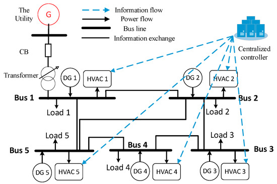
Figure 1.
The microgrid structure under study.
HVAC units are the key components under study in the system. A HVAC unit can be either an AC inverter-based air conditioner or a DC inverter-based air conditioner, which employs AC motor or DC motor to drive the compressor, respectively. Figure 2 shows the schematic of a typical AC inverter-based air conditioner, demonstrating how the controller algorithms are integrated into power conversion of the HVAC system.
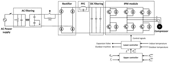
Figure 2.
The schematic diagram of a typical AC inverter HVAC (heating ventilation air conditioning) system.
In Figure 2, the power conversion circuit aims to achieve AC-DC-AC, which consists of an AC filtering module, a rectifier, a power factor control (PFC) circuitry, a DC filtering module, and an intelligent power module (IPM). Firstly, a stable DC voltage is obtained by connecting capacitors along with a PFC in the current path after the rectifier. The IPM module is utilized to convert DC to AC regulated by the PWM (pulse width modulation) signals as controlled to drive the compressor. There are two controllers in the HVAC unit. The upper controller implements the distributed algorithm and generates reference frequency and power signals () in response to the local power mismatch () and power constraint of the HVAC unit (, ) and frequency from the neighboring HVAC (). Provided that the indoor and outdoor temperatures, frequency and power reference signals are given, the lower controller then generates PWM pulses to drive the IGBT (insulated-gate bipolar transistor) in the IPM module to ensure the compressor to work under a desirable frequency. Furthermore, the lower controller adjusts the operation state of the expansion valve and outdoor machine to assist its operation.
3. Preliminaries
In this section, the preliminary knowledge about graph theory and consensus algorithm is given.
3.1. Graph Theory
The communication topology among agents in MAS can be described with an undirected graph , with a non-empty node set and a finite edge set denoted by . As for an undirected graph, the edge presents vertex and enabling to exchange information with each other. Nodes and are regarded as the neighbor nodes. In this paper, the self-loop edges are not considered in the topology. Let denote the union of neighbor vertexes for vertex . If each node in an undirected graph has connection with any other nodes, the graph is called a strongly connected graph. Consider Figure 1, where each local bus is modelled as a node. The thin black solid lines signify the information interaction between neighboring nodes and hence, they form the communication topology. Clearly, the topology under Figure 1 is a strongly connected undirected graph. Mathematically, the topology can be described as a matrix to explain the interaction among agents, which will be demonstrated in the subsequent section.
3.2. Consensus Algorithm
Considering a discrete-time multi-agent system, the information update of each agent relies on the current state of itself and its neighbor agents. Based on consensus algorithm, it is written as:
where is the state of agent at the iteration , is communication weighting coefficient between vertex and . Equation (1) can be rewritten in terms of matrices as below:
where matrix corresponds to an undirected graph . Different methods have been used to define matrix such as those used in references [8,9,17]. Here, the Vicsek model is adopted to define as follows [27]:
where represents the number of elements in set . It can be seen that matrix associated with a strongly connected graph is a positive doubly stochastic matrix, where the sum of coefficients in rows and columns are both equal to one. Matrix satisfies the following conditions [17,18].
- and , where is a column vector of all ones.
- is a nonnegative, doubly stochastic matrix with the condition 1. Based on the definition in [28], is spectral radius of matrix , with the rest of eigenvalues being positive.
- The average consensus is achievable based on initial conditions of all agents, if the graph is strongly connected. The consensus state is calculated by and denotes initial condition for agent .
The above properties will be utilized in Section 5 for proof of DSM distributed algorithm.
4. HVAC-Based DSM Problem Formulation
Considering an IEEE -bus system to construct a microgrid system, the active power balance model without transmission loss can be expressed as:
where is the distributed power generation at the -th local bus, denotes the non-adjustable load demand at bus , and is the total power mismatch for the entire microgrid system. An appropriate dispatching strategy therefore needs to be implemented to share the total power mismatch by regulating power consumption of the HVAC unit such that
When power consumption constraints for each HVAC are applied, the objective of coordinating multiple HVAC units is to minimize the cost function:
where , are lower and upper power constraints for the -th HVAC unit, respectively.
A HVAC system is physically composed of a compressor, an evaporator, condenser and expansion valves, sensors, electrical control parts and a central controller. It is the central controller, i.e., the lower controller as shown in Figure 2, that provides appropriate control signals to track the compressor power reference. Figure 3 shows the performance curves of a typical HVAC, demonstrating the relationship of operating frequency of the compressor against the cooling load, COP (Coefficient of Performance) and power consumption, respectively. The operating frequency increases with the increment of the cooling load. Then, the expansion valve will open more to ensure the HVAC to operate at an optimal COP value. Consequently, the power consumption of the compressor increases with the growth of the operating frequency. A series of performance testing carried out in [23] indicate that the compressor power consumption only relies on the operating frequency and is independent of the temperature.
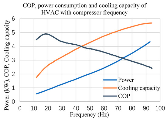
Figure 3.
COP, power consumption and cooling capacity of the HVAC against the compressor operating frequency [24].
The relationship between the power consumption and compressor frequency can be numerically fitted by a first-order function, without considering the power constraints:
where is the operating frequency of the associated compressor, and and are a pair of model coefficients with respect to -th HVAC unit. Physically, and denote load ramp rates and initial power of the HVAC unit, respectively.
Assume there are HVAC units in a microgrid system, then according to Equations (7) and (9), all frequency signals will eventually converge to an optimal common value , which is calculated as:
The associated power consumption for each HVAC is therefore:
Considering power constraints on HVAC, the frequency can be specified as:
Let define as a subset of the HVAC units where the power consumption is saturated, in order to achieve the optimal assignment, we have:
The power consumption for each HVAC can be described as:
The results obtained in Equation (14) are the solution to the DSM problem as formulated in Equations (6)–(8) with HVAC power constraints being considered.
5. Distributed Algorithm for DSM
In this section, we present a distributed cooperative algorithm by incorporating the HVAC model in order to address DSM problem in a standalone microgrid system. The main objective is to obtain a desired frequency and power reference for HVAC to compensate local power mismatch. The convergence proof for the proposed algorithm under fixed topology and dynamic topologies are given. Then, a two-level control scheme employed by HVAC is presented to demonstrate how the algorithm is implemented.
5.1. Under Fixed Topology
Let and be the operating frequency and power consumed for the -th HVAC at the iteration , respectively. denotes the power mismatch estimated between the local power generation and local load demand at bus . is a positive coefficient affecting the convergence speed. The discrete time distributed algorithm is described as
Remark 1.
The update of
in the Equation (15) is obtained based on collaborative efforts of all neighboring agents of the -th HVAC and its current state. The stability of the algorithm mainly relies on consensus term which is determined by the associated communication topology. The surplus term
provides a feedback mechanism to ensure the convergence and is called state feedback gain, which dominates the convergence speed of when converging to optimal
.
Consider the initial conditions:
Let be any value within the power constraint boundary, and total initial power consumed by HVAC devices is .
Equations (15)–(17) can be rewritten in a matrix form as follows:
where , , , are column vectors of , , , , respectively, with . Define , . Since , as defined by Equation (3), is a doubly stochastic matrix, we obtain from Equation (20):
It indicates the summation can be preserved for all iteration . With the initial condition, we have . If when for , the power imbalance problem is solved for each bus.
The Equations (19)–(21) can be reformatted as a matrix form:
Note that matrix has negative entries due to the presence of . Thus, the characteristic of the nonnegative matrix based on the spectrum of cannot be directly utilized. Here, matrix perturbation theory is employed to verify the convergence of algorithm with a certain graphical condition of the topology being applied [29].
Theorem 1.
Suppose a communication digraph is strongly connected, each agent can achieve the average consensus with the distributed algorithm described in Equations (15)–(17), if the feedback gain is properly small [15].
Proof of Theorem 1.
In Equation (23), the matrix can be regarded as a deterministic matrix perturbed by a parameter matrix. The derivatives of eigenvalues for
are verified to be non-positive, given a sufficiently small parameter matrix . The convergence proof of the algorithm can be referred in [15].
Now considering power constraints on HVAC, Equation (17) is then revised to:
where , . With the same initial values as given in Equations (18) and (23), it is then revised to:
where with
The revised Equations (24)–(26) also satisfy Theorem 1.
5.2. Under Time-Varying Topology
Assuming the communication network in the MAS is time varying, the Equations (15) and (16) need to be improved to accommodate the average consensus in a dynamic topology.
where the switching parameter , if the , or otherwise . Let us define as also a doubly stochastic matrix as . This means that the agent updates its current state and may only rely on its surplus term, if there is no direct information from in-neighbors during the time subinterval. A matrix format is expressed as:
Theorem 2.
The revised Equations (27) and (28) can solve the average consensus under a dynamically changing interaction topology if the union of the directed graph across each interval is strongly connected.
As known, the state matrix in Equation (29) fails to be divided into a deterministic matrix and parameter matrix due to the appearance of . The matrix perturbation theory is thus not applicable to prove a dynamic topology. The convergence proof of Equation (29) is now conducted based on the Lyapunov-type argument.
In order to design a Lyapunov candidate function, we introduce the maximum and minimum frequency state and with regard to Equation (27) satisfying:
As demonstrated in reference [30], the minimum value is a non-decreasing variable for each iteration. It satisfies , if is the convergence value. When , all agents satisfy average consensus condition at which and . The final equilibrium point will be , where is a column vector that all elements must be zero.
Similar to the derivation in fixed topology case as Equation (22), we then obtain:
This implies that is a constant quality for all . Given the initial condition , the steady state value for each agent converges to , where the scalar . We define a set to describe the change of states when they approach and converge to the consensus point.
Remark 2.
Suppose that and are positive bounded functions with respect to the equilibrium point. There exist finite times satisfies that each state meets.
Then, the network of agents achieves uniform average consensus.
Now, we introduce a Lyapunov candidate function as below:
Clearly, is a continuous and bounded function with respect to , because both and are restricted. With the definition of both terms as mentioned above, is positive definite when , while , if the state converges to the consensus point .
Assuming that κ denotes switching times occurring time interval , we consider an auxiliary function , where , which satisfies:
where the function experiences all possible sequences ,, satisfying Equation (29). Thus, is a pair of reachable state from . From Equation (33), if , the only solution is and , thus , which indicates the system reaches the average consensus point. Then, we introduce Lemma 1 as below, in order to demonstrate the positive definite property of the , when ).
Lemma 1.
If a dynamic digraph is jointly strongly connected during each time interval, there is a finite switching times happens in , when and both satisfy the strictly positive condition.
Since the preconditions of positive definite property of and are based on the non-decreasing property of minimum state, it satisfies . The proof of Lemma 1 relies on the graphical condition of jointly strongly connected topology, dynamic state information and surplus updating as described in Equations (27) and (28), which is organized by two steps. Firstly, suppose that some nodes in a network have positive surplus, all nodes will then have positive surplus in a finite time, due to a jointly strongly connected graph. Secondly, by using the positive surplus, the node having a minimum state of the updated graph will not decrease with the non-negative property of the minimum state. More detailed proof can be found in [30].
Proof of Theorem 2.
Assume that
denotes a dynamic communication network under a multi-agent system, which is jointly strongly connected. We then define a Lyapunov candidate function (Equation (32)) and an auxiliary function (Equation (33)) with both satisfying the condition in Lemma 1. According to second method of Lyapunov, the stability of presented Equations (27) and (28) is verified and a uniform average consensus is achievable.
5.3. Algorithm Implementation
It is worth emphasizing that the state feedback gain is a crucial parameter that dominates the stability and convergence rate of the distributed algorithm. Figure 4 illustrates the change of convergence time with feedback gain under a fixed topology. It can be clearly seen that the convergence time decreases exponentially when . Then, the convergence rate is growing slightly when rises to 9 and the system becomes unstable when . Apparently, the optimal value of lies at the corner point of the curve, which is 3.6 resulting in a fastest consensus time and 35 iterations associated with settling time. Similar trends are also found for the revised algorithm under the time-varying topology.
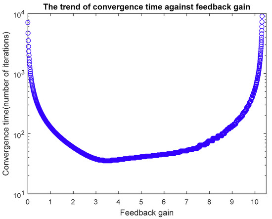
Figure 4.
Convergence time with varying feedback gain.
The algorithms are implemented based on the proposed MAS framework. The control scheme for each agent is described in Figure 5. The upper controller determines the desired frequency and calculates the power reference for each HVAC to operate. It is composed of five function blocks. The initialization and measurement block define the initial condition as specified in Equation (18) and specifies the local power mismatch. Power constraint block specifies the operating power range for each HVAC, as indicated in Equation (24). Communication block exchanges information of frequency and the estimated power mismatch with neighboring agents. The optimal frequency discovery block updates its state according to Equation (15). Local information update block calculates the HVAC power consumption and local power mismatch reference signals, as calculated by Equations 16 and 17 and provides them to the lower controller of the HVAC. The lower controller of the HVAC varies its control signal by tracking the frequency and power reference signals, as described in Section 2.
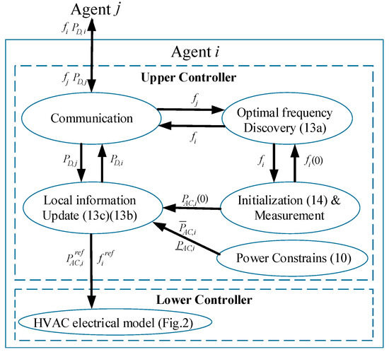
Figure 5.
Block diagram of a two-level control scheme for MAS.
In summary, the consensus Algorithm 13 under a fixed communication topology with/without power constraints are firstly presented. The algorithm is then modified to address the case under time-varying interaction topology. The stability of the revised Algorithm 21 with its stable condition is proved by Lyapunov stability theorem, where a Lyapunov candidate function (Equation (32)) and an auxiliary function (Equation (33)) are proposed to support the proof.
6. Simulation Results
In this section, the feasibility of the proposed Algorithms 13 and 19 for power constraint and unconstraint conditions are firstly studied in Case 1 and Case 2, respectively. Then, the power unconstraint case is revised to test the time-varying power generation scenarios of renewable energy generators, which is shown in Case 3. In Case 4, robustness of the algorithms is discussed when the HVAC is considered to be broken down or removed from the microgrid system in order to evaluate the anti-damage capability of the microgrid. The performance of the network with time-varying topology to verify the Algorithm 21 is lastly assessed and demonstrated in Case 5.
The microgrid system under test, as shown in Figure 1, is an IEEE 5-bus system. Each bus has a distributed generator, HVAC unit and other uncontrollable loads. Suppose that the system operates in island mode, which has no power exchange with the main grid. The interaction topology matrix regarding the communication topology can be determined with Equation (3). Table 1 gives the parameters of HVAC capacities and power generation of local buses. The feedback gain for each bus is assumed identical to simplify the problem. Based on Equation (18) and HVAC specifications, initial values are selected as Hz, kW, kW. Referred to the trend of convergence rate against feedback gain as shown in Figure 4, is adopted in the case studies unless otherwise specified. All of simulations are performed with MATLAB/SIMULINK.

Table 1.
Parameter setting of HVAC unit in microgrid system.
6.1. Case Study 1: Without HVAC Power Constraints
In this case study, power constraints of HVAC units are not imposed. Figure 6 shows the update of frequency signal, power consumption, local bus supply-demand mismatch and total energy consumption (as demanded to be 11.55 kW). After 35 iterations, local power mismatch goes to zero, as shown in Figure 6c, while power consumed matches the power supplied as shown in Figure 6d. The operating frequency of all HVAC units converges to a common value Hz, as seen from Figure 6a. The power consumption for each HVAV is kW, kW, kW, kW, and kW, respectively, as seen from Figure 6b. It is noted that the power output of the HVAC 1 should be saturated if power constraints are applied.
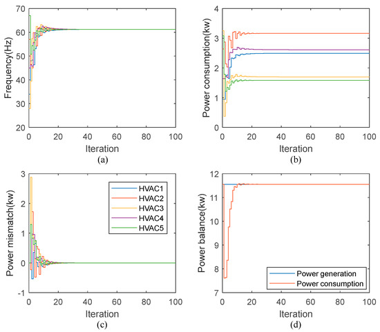
Figure 6.
Results without power constraints: (a) Frequency; (b) HVAC power consumption; (c) Estimated power mismatch and (d) Power balance. Note that legend in (c) is also valid for (a,b).
6.2. Case Study 2: With HVAC Power Constraints
Following results in Case 1, Figure 7 illustrates results for the case considering HVAC power constraint. After 35 iterations, the units converge to a new frequency Hz. The power consumption for each HVAC unit is kW, kW, kW, kW, kW, respectively. Note that the power of HVAC 1 becomes saturated now after 5 iterations and the optimal frequency has a slight increase from 60.2061 Hz to 63.6146 Hz. The unsaturated HVAC units share more power with the growing frequency to compensate the effect of the saturated HVAC device. However, the performance of local power mismatch and power balance for the entire system is not affected, as can be seen from Figure 7c,d.
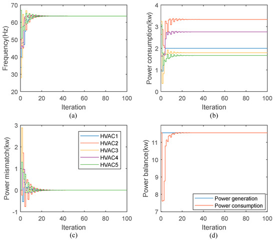
Figure 7.
Results with power constraints: (a) Frequency; (b) HVAC power consumption; (c) Estimated power mismatch and (d) Power balance. Note that legend in (c) is also valid for (a,b).
6.3. Case Study 3: Time-Varying Power Generation
This case investigates performance of the proposed algorithms under the time-varying power generation, meaning there is a dynamic change for the supply-demand mismatch due to the presence of intermittent and uncontrollable renewable generators. We purposely increase 5 kW power generation () at 1st local bus at the 50th iteration.
As can be seen from Figure 8, before the 50th iteration, their transient response is the same as in Case 2. After the 50th iteration, consensus frequency increases from 63.61 Hz to 94.12 Hz to accommodate this power generation increase. The consensus power consumed for HVAC devices are now kW, kW, kW, kW, kW, respectively. These non-saturated HVAC units take more power to share the increased power generation due to power being saturated by those units (HVAC 1 and 4).
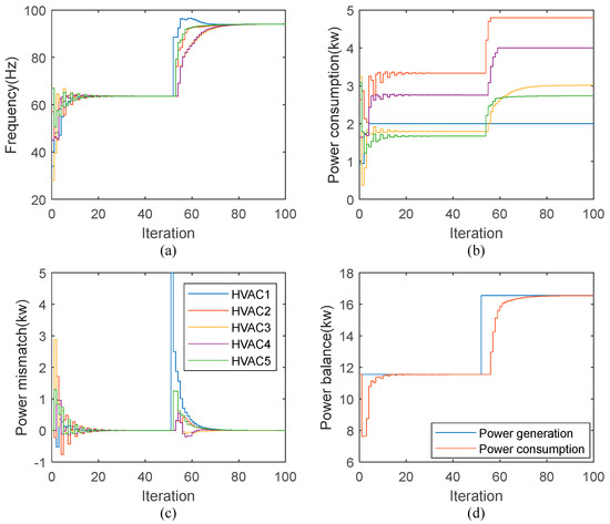
Figure 8.
Results of time-varying power generation: (a) Frequency; (b) HVAC power consumption; (c) Estimated power mismatch and (d) Power balance. Note that legend in (c) is also valid for (a,b).
6.4. Case Study 4: Anti-Damage Test
In this case, HVAC breakdown is emulated to assess the robustness of the proposed algorithm. It is assumed that at the 50th iteration, HVAC 1 fails, where a zero power is assigned to HVAC 1 before the next iteration. Thus, we define . The consensus frequency value increases up to 73.37 Hz due to the higher energy share for the remaining four HVACs (Figure 9a). Note that the simulated frequency is specified as a reference value. Practically, the faulty HVAC unit would not be able to operate at the specified frequency. The power consumed is kW, kW, kW, kW, kW (Figure 9b). The performance shows that all power demands to HVAVs are still within their power boundaries. The balance between the total power generation and load demand can still be achieved after the breakdown fault of a HVAC appears.
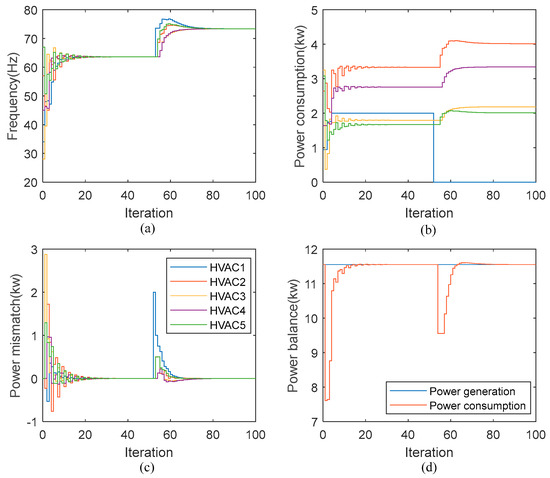
Figure 9.
Results of anti-damage test: (a) Frequency; (b) HVAC power consumption; (c) Estimated power mismatch and (d) Power balance. Note that legend in (c) is also valid for (a,b).
6.5. Case Study 5: Under the Time-Varying Topology
In order to identify the effectiveness of the algorithm under the time-varying topology, we suppose the communication among HVAC units is a dynamic network in this case. Let define that the interaction topology is switching randomly within the set at each iteration, as shown in Figure 10, where the associated matrices are given. Apparently, the time-varying topology is a jointly strongly connected network, which satisfies the consensus condition. The results show that values at steady-state conditions are the same as those in Case Study 1 (Figure 11a,b). However, the stability is not able to be achieved until the 50th iteration, due to exchange of the intermittent information. Therefore, the algorithm presented in Equations (27) and (28) under a dynamic topology will restrict the efficiency of information broadcast and thus increase the convergence time.
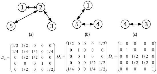
Figure 10.
Switching topologies and corresponding Laplacian matrix.
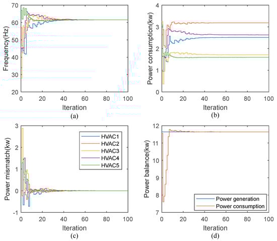
Figure 11.
Convergence performance of consensus algorithm under dynamic topology: (a) Frequency; (b) HVAC power consumption; (c) Estimated power mismatch and (d) Power balance. Note that legend in (c) is also valid for (a,b).
7. Conclusions
This paper investigates the energy dispatch problem in an autonomous microgrid system. The proposed control scheme shows the following advances.
- i
- The aggregated HVAC devices effectively solve the supply-demand imbalance in the microgrid system whilst alternatively alleviate the capacity and quantity of energy storage devices.
- ii
- An advanced consensus algorithm has been developed for the time-varying topology with more relaxed graphic conditions than the consensus condition under the fixed topology.
- iii
- The relationship between the state feedback gain and convergence time is investigated in order to obtain an optimal feedback gain to be applied in the case studies.
- iv
- The simulation results demonstrate the feasibility, dynamic and robustness of the proposed distributed control algorithms.
It is worth noting that this work focuses on varying the power consumption of HVAC devices to compensate the local supply-demand mismatch. Hence, the cooling capacity and resident comfortable level have not been taken into account. User satisfaction is relatively sacrificed to achieve zero power mismatch. Therefore, in the next stage, a multi-objective optimization problem will be formulated in order to accommodate the resident comfortable level within an acceptable level. Furthermore, the renewable power forecasting can be incorporated into control protocols to implement a preschedule energy dispatch scheme for individual HVAC units.
Author Contributions
Conceptualization, J.M. and X.M.; methodology, J.M. and X.M.; software, J.M.; validation, J.M. and X.M.; formal analysis, J.M. and X.M.; investigation, J.M.; resources, J.M.; data curation, J.M.; writing—original draft preparation, J.M.; writing—review and editing, J.M., X.M. and S.I.; visualization, J.M. and X.M.; supervision, X.M. and S.I.; project administration, X.M. and S.I.; funding acquisition, J.M. and X.M.
Funding
This project was partially funded by European Regional Development Fund (ERDF) and Entrust Microgrid LLP.
Acknowledgments
The authors express their great appreciation to Metoffice by providing online weather forecast data.
Conflicts of Interest
The authors declare no conflict of interest.
Abbreviations
| MAS | Multi-agent system |
| HVAC | Heating ventilation air conditioning |
| DSM | Demand side management |
| TCL | Thermostatically controlled load |
| BESS | Battery energy storage system |
| DG | Distributed generator |
| PFC | Power factor control |
| IPM | Intelligent power module |
| PWM | Pulse width modulation |
| COP | Coefficient of Performance |
References
- Hug, G.; Kar, S.; Wu, C. Consensus + Innovations Approach for Distributed Multiagent Coordination in a Microgrid. IEEE Trans. Smart Grid 2015, 6, 1893–1903. [Google Scholar] [CrossRef]
- Palensky, P.; Dietrich, D. Demand Side Management: Demand Response, Intelligent Energy Systems, and Smart Loads. IEEE Trans. Ind. Inform. 2011, 7, 381–388. [Google Scholar] [CrossRef]
- Guerrero, J.; Castilla, M.; Vasquez, J.C.; Miret, J.; De Vicuna, L.G. Hierarchical Control of Intelligent Microgrids. IEEE Ind. Electron. Mag. 2010, 4, 23–29. [Google Scholar]
- Deng, R.; Yang, Z.; Chow, M.-Y.; Chen, J. A Survey on Demand Response in Smart Grids: Mathematical Models and Approaches. IEEE Trans. Ind. Inform. 2015, 11, 570–582. [Google Scholar] [CrossRef]
- He, M.-F.; Zhang, F.-X.; Huang, Y.; Chen, J.; Wang, J.; Wang, R. A Distributed Demand Side Energy Management Algorithm for Smart Grid. Energies 2019, 12, 426. [Google Scholar] [CrossRef]
- Nikmehr, N.; Najafi-ravadanegh, S.; Khodaei, A. Probabilistic optimal scheduling of networked microgrids considering time-based demand response programs under uncertainty Time of Use. Appl. Energy 2017, 198, 267–279. [Google Scholar] [CrossRef]
- Castillo-Cagigal, M.; Matallanas, E.; Caamaño-Martín, E.; Martín, Á.G. SwarmGrid: Demand-Side Management with Distributed Energy Resources Based on Multifrequency Agent Coordination. Energies 2018, 11, 2476. [Google Scholar] [CrossRef]
- Heydari, R.; Khayat, Y.; Naderi, M.; Anvari-Moghaddam, A.; Dragicevic, T.; Blaabjerg, F. A Decentralized Adaptive Control Method for Frequency Regulation and Power Sharing in Autonomous Microgrids. In Proceedings of the IEEE 28th International Symposium on Industrial Electronics (ISIE), Vancouver, BC, Canada, 12–14 June 2019; pp. 2427–2432. [Google Scholar]
- Anvari-Moghadam, A.; Shafiee, Q.; Vasquez, J.C.; Guerrero, J.M.; Anvari-Moghaddan, A. Optimal adaptive droop control for effective load sharing in AC microgrids. In Proceedings of the IECON 2016-42nd Annual Conference of the IEEE Industrial Electronics Society, Florence, Italy, 24–27 October 2016; pp. 3872–3877. [Google Scholar]
- Vahedipour-Dahraie, M.; Najafi, H.R.; Anvari-Moghaddam, A.; Guerrero, J.M. Optimal scheduling of distributed energy resources and responsive loads in islanded microgrids considering voltage and frequency security constraints. J. Renew. Sustain. Energy 2018, 10, 025903. [Google Scholar] [CrossRef]
- Zhang, W.; Lian, J.; Chang, C.-Y.; Kalsi, K. Aggregated Modeling and Control of Air Conditioning Loads for Demand Response. IEEE Trans. Power Syst. 2013, 28, 4655–4664. [Google Scholar] [CrossRef]
- Hlava, J.; Zemtsov, N. Aggregated control of electrical heaters for ancillary services provision. In Proceedings of the 2015 19th International Conference on System Theory, Control and Computing (ICSTCC), Cheile Gradistei, Romania, 14–16 October 2015; pp. 508–513. [Google Scholar]
- Tindemans, S.H.; Trovato, V.; Strbac, G. Decentralized Control of Thermostatic Loads for Flexible Demand Response. IEEE Trans. Control Syst. Technol. 2015, 23, 1685–1700. [Google Scholar] [CrossRef]
- Wu, X.; He, J.; Xu, Y.; Lu, J.; Lu, N.; Wang, X. Hierarchical Control of Residential HVAC Units for Primary Frequency Regulation. IEEE Trans. Smart Grid 2018, 9, 3844–3856. [Google Scholar] [CrossRef]
- Wang, R.; Li, Q.; Zhang, B.; Wang, L. Distributed Consensus Based Algorithm for Economic Dispatch in a Microgrid. IEEE Trans. Smart Grid 2019, 10, 3630–3640. [Google Scholar] [CrossRef]
- Yang, S.; Tan, S.; Xu, J.-X. Consensus Based Approach for Economic Dispatch Problem in a Smart Grid. IEEE Trans. Power Syst. 2013, 28, 4416–4426. [Google Scholar] [CrossRef]
- Zhang, Z.; Chow, M.-Y. Incremental cost consensus algorithm in a smart grid environment. In Proceedings of the 2011 IEEE Power and Energy Society General Meeting, Detroit, MI, USA, 24–28 July 2011; pp. 1–6. [Google Scholar]
- Xu, Y.; Zhang, W.; Hug, G.; Kar, S.; Li, Z. Cooperative Control of Distributed Energy Storage Systems in a Microgrid. IEEE Trans. Smart Grid 2015, 6, 238–248. [Google Scholar] [CrossRef]
- Zhao, T.; Ding, Z. Cooperative Optimal Control of Battery Energy Storage System under Wind Uncertainties in a Microgrid. IEEE Trans. Power Syst. 2018, 33, 2292–2300. [Google Scholar] [CrossRef]
- Thomas, M.; Hredzak, B.; Agelidis, V. Distributed Cooperative Control of Microgrid Storage. IEEE Trans. Power Electron. 2015, 30, 2780–2789. [Google Scholar]
- Rahman, M.; Oo, A. Distributed multi-agent based coordinated power management and control strategy for microgrids with distributed energy resources. Energy Convers. Manag. 2017, 139, 20–32. [Google Scholar] [CrossRef]
- Vahedipour-Dahraie, M.; Rashidizaheh-Kermani, H.; Najafi, H.R.; Anvari-Moghaddam, A.; Guerrero, J.M. Coordination of EVs Participation for Load Frequency Control in Isolated Microgrids. Appl. Sci. 2017, 7, 539. [Google Scholar] [CrossRef]
- Shao, S.; Shi, W.; Li, X.; Chen, H. Performance representation of variable-speed compressor for inverter air conditioners based on experimental data. Int. J. Refrig. 2004, 27, 805–815. [Google Scholar] [CrossRef]
- Park, Y.C.; Kim, Y.C.; Min, M.-K. Performance analysis on a multi-type inverter air conditioner. Energy Convers. Manag. 2001, 42, 1607–1621. [Google Scholar] [CrossRef]
- Ma, K.; Hu, G.; Spanos, C.J. Energy Management Considering Load Operations and Forecast Errors With Application to HVAC Systems. IEEE Trans. Smart Grid 2018, 9, 605–614. [Google Scholar] [CrossRef]
- Ma, J.; Ma, X. A review of forecasting algorithms and energy management strategies for microgrids. Syst. Sci. Control Eng. 2018, 6, 237–248. [Google Scholar] [CrossRef]
- Ren, W.; Beard, R.W. Distributed Consensus in Multi-Vehicle Cooperative Control; Springer: Berlin, Germany, 2008. [Google Scholar]
- Horn, R.; Johnson, C. Matrix Analysis; Cambridge University Press: Cambrige, UK, 1985. [Google Scholar]
- Cai, K.; Ishii, H. Average consensus on general strongly connected digraphs. Automatica 2012, 48, 2750–2761. [Google Scholar] [CrossRef]
- Cai, K.; Ishii, H. Average Consensus on Arbitrary Strongly Connected Digraphs With Time-Varying Topologies. IEEE Trans. Autom. Control 2014, 59, 1066–1071. [Google Scholar] [CrossRef]
© 2019 by the authors. Licensee MDPI, Basel, Switzerland. This article is an open access article distributed under the terms and conditions of the Creative Commons Attribution (CC BY) license (http://creativecommons.org/licenses/by/4.0/).