Article

Research on the Prediction Method of Centrifugal Pump Performance Based on a Double Hidden Layer BP Neural Network

1
Department of Energy and Power Engineering, Lanzhou University of Technology, Lanzhou 730050, China
2
Key Laboratory of Fluid Machinery and Systems, Lanzhou University of Technology, Lanzhou 730050, China
3
Department of Electrical and Information Engineering, Lanzhou University of Technology, Lanzhou 730050, China
4
Department of Architecture and Transportation Engineering, Guilin University of Electronic Technology, Guilin 541004, China
*
Authors to whom correspondence should be addressed.
Energies 2019, 12(14), 2709; https://doi.org/10.3390/en12142709
Submission received: 31 May 2019 / Revised: 10 July 2019 / Accepted: 12 July 2019 / Published: 15 July 2019
(This article belongs to the Special Issue Mathematical Modelling of Energy Systems and Fluid Machinery)

Abstract

:
With the aim of improving the shortcomings of the traditional single hidden layer back propagation (BP) neural network structure and learning algorithm, this paper proposes a centrifugal pump performance prediction method based on the combination of the Levenberg–Marquardt (LM) training algorithm and double hidden layer BP neural network. MATLAB was used to establish a double hidden layer BP neural network prediction model to predict the head and efficiency of a centrifugal pump. The average relative error of the head between the experimental and prediction obtained by the double hidden layer BP neural network model was 4.35%, the average relative error of the model prediction efficiency and the experimental efficiency was 2.94%, and the convergence time was 1/42 of that of the single hidden layer. The double hidden layer BP neural network model effectively solves the problems of low learning efficiency and easy convergence into local minima—issues that were common in the traditional single hidden layer BP neural network training. Furthermore, the proposed model realizes hydraulic performance prediction during the design process of a centrifugal pump.

1. Introduction

The performance prediction of centrifugal pumps has become an indispensable part of the optimization design of centrifugal pumps. At present, the traditional prediction methods mainly include computational fluid dynamics (CFDs) numerical simulation methods, and empirical formulas [1]. When the CFDs method is used to predict the performance of a centrifugal pump, the performance prediction error of centrifugal pumps is usually more than 5%, due to the fact that the mechanical loss and partial volume loss of the centrifugal pump are ignored. Meanwhile, empirical formulas can be used to predict the efficiency of a centrifugal pump under the design parameters, but they cannot effectively predict the actual efficiency of an impeller with the same design parameters and different structural parameters (blade number, blade angle, etc.). Table 1 shows the empirical relationship of the disc loss with different specific speeds of a centrifugal pump. The disc loss is nearly inversely proportional to the specific speed [2]. Otherwise, the disc loss is difficult to test and apply in the pump system.
Testing the performance of a centrifugal pump by the experimental method includes three steps: The design, manufacturing, and performance test of the prototype pump. However, this method has some shortcomings, such as tedious measurement process, high cost, and a long research and development cycle. Therefore, it is generally not used as the preferred method to predict the performance during the design process of pumps nowadays.
In recent years, the artificial neural network (ANN) method has often been used to solve uncertain or nonlinear control problems owing to its advantages of strong adaptability, high accuracy, precise function approximation ability, and nonlinear mapping ability. In ANN, the nonlinear mapping relationship is built between the input and output of sample data through the self-learning ability of each neuron. It has the characteristics of large-scale parallel processing, fault tolerance, self-organization and self-adaptation ability, and strong associative function. Therefore, it has been applied in many fields for performance prediction, target recognition, intrusion detection, on-line supervisory control, fault diagnosis, etc. Li et al. [3] proposed a method of combining a chaos algorithm with a genetic algorithm to overcome the shortcomings of the neural network for gesture recognition, and used the optimal result as the initial weight and threshold of the BP neural network to identify gestures. Simulation and experimental results showed that this method has better real-time accuracy for gesture recognition. Peng et al. [4] proposed a vehicle and personnel identification method based on an improved neural network—that is, the seismic signals of moving objects are processed and analyzed to obtain eigenvectors—so as to realize good classification. Experimental results showed that the method has better recognition accuracy and effectiveness.
The ANN method has a shorter prediction cycle and lower cost compared with the experimental method. Moreover, it can predict the hydraulic performance during the design process of a centrifugal pump, as it is forward-looking and time-sensitive, and provides a new idea for the efficient performance prediction of centrifugal pumps. Ne et al. [5] first applied the BP algorithm in ANN for the performance prediction of a centrifugal pump. In the training process, the method constantly modified the weight value using the gradient fastest descent method, and the weight value changed along the negative gradient direction of the error function. The maximum predicted the deviation of the head and efficiency to be 7% and 8%, respectively, which shows the feasibility of pump performance prediction based on the ANN method. Yao et al. [6] used the BP neural network to predict the centrifugal pump head, and the training function was learned by the gradient descent method. The highly nonlinear mapping between the geometric parameters’ input of the transition parts and the performance output of the centrifugal pump was realized through the self-application and learning function of the neural network. Cong et al. [7] used the Bayesian regularization algorithm to predict the performance of a single stage centrifugal pump hydraulic model, in which the regularization method improved the generalization ability by modifying the training performance function of the neural network. They found that the error of performance prediction with the improved neural network was lower than 6%. Jiang et al. [8] considered that the CFD numerical simulation method directly used to predict the performance of a centrifugal pump will greatly increase the calculation cost, and the design cycle will also become longer. Therefore, they used the combination of CFDs simulation and the BP neural network to predict the efficiency of the centrifugal pump impeller. BP neural network technology was used to establish an approximate proxy model between the influencing factors and the response value, and the optimized hydraulic model of the centrifugal pump was given. Otherwise, the method was limited to the optimization design of the centrifugal pump impeller with a lower specific speed.
The above studies on the performance prediction of centrifugal pumps are all based on the single hidden layer BP neural network. Due to the simple structure of the single hidden layer BP neural network, it is impossible to extract more characteristic information of input parameters, and the prediction of centrifugal pump performance faces problems, such as small coverage and low robustness. Considering that a deeper network depth will result in network redundancy and the convergence time of the network will become longer, this will lead to an inaccurate performance prediction of the centrifugal pump. Therefore, it is necessary to establish an appropriate method to increase the network depth and accelerate the convergence of the deep BP neural network to improve the prediction accuracy of centrifugal pump performance.
In recent years, the LM algorithm has been favored by domestic and overseas scholars [9,10,11,12]. It is a classical nonlinear numerical optimization algorithm that combines the advantages of the gradient descent method and the Gauss-Newton method. Moreover, it has the local convergence of the Gauss-Newton method and the global characteristics of the gradient descent method. The fast convergence of the Gauss-Newton method is adopted when the solution is near to the optimal solution, and the convergence characteristic is achieved by adaptively adjusting the damping factor. The approximate second-order derivative information is used to achieve the ability of superlinear convergence near the optimal solution, which has a higher iterative convergence speed and accelerates the convergence of the neural network. The robustness of the gradient descent method is adopted when the solution is far from the optimal solution. That is, when the input information or the neural network has finite perturbation, the neural network can still maintain the stability characteristics from the input to the output relationship to obtain reliable solutions, thus solving problems, such as the poor numerical stability of the neural network. This approach has thus been widely applied to various research fields.
Wang [13] designed a new intrusion detection model based on the LM-BP neural network to address the issues of the traditional BP neural network, such as slow convergence speed, the tendency to fall into local minima, and high cost of computation. Through further research of the neural network and intrusion detection systems, the comparative experimental results showed that the new model combines the advantages of anomaly and misuse detection. It can quickly detect new intrusions as well as reduce the false alarm rate and missed alarm rate. Zhao et al. [14] applied the LM algorithm neural network with the learning rate for on-line supervisory control. Compared with the traditional forward neural network BP, the new control strategy can improve the operation speed and the local minima. It can improve the tracking performance of the servo system with an unknown load disturbance. The search direction can be optimized by the LM-BP neural network and has been applied to transformer fault diagnosis [15]. Through test and analysis, not only was the convergence speed accelerated, but the accuracy was also greatly improved. The study results showed that the positive rate of the fuzzy fault diagnosis reached 92.5%; the verified method could improve the transformer fault diagnosis performance.
To sum up, the nonlinear relationship between the hydraulic performance and the structural parameters of the impeller is so complex that the actual efficiency of the impeller is difficult to predict with different structural parameters, whether by CFDs or empirical methods. On the other hand, the double hidden layer BP neural network can enhance the mapping ability of the complex relationship between the input and output of the system, and has stronger approximation and fault tolerance abilities than the single hidden layer BP neural network [16]. So, the combination of the LM algorithm and double hidden layer BP neural network can be used to predict the performance of centrifugal pumps rapidly and precisely for use in strong nonlinear engineering prediction fields, such as intrusion detection, on-line supervisory control, and transformer fault diagnosis.

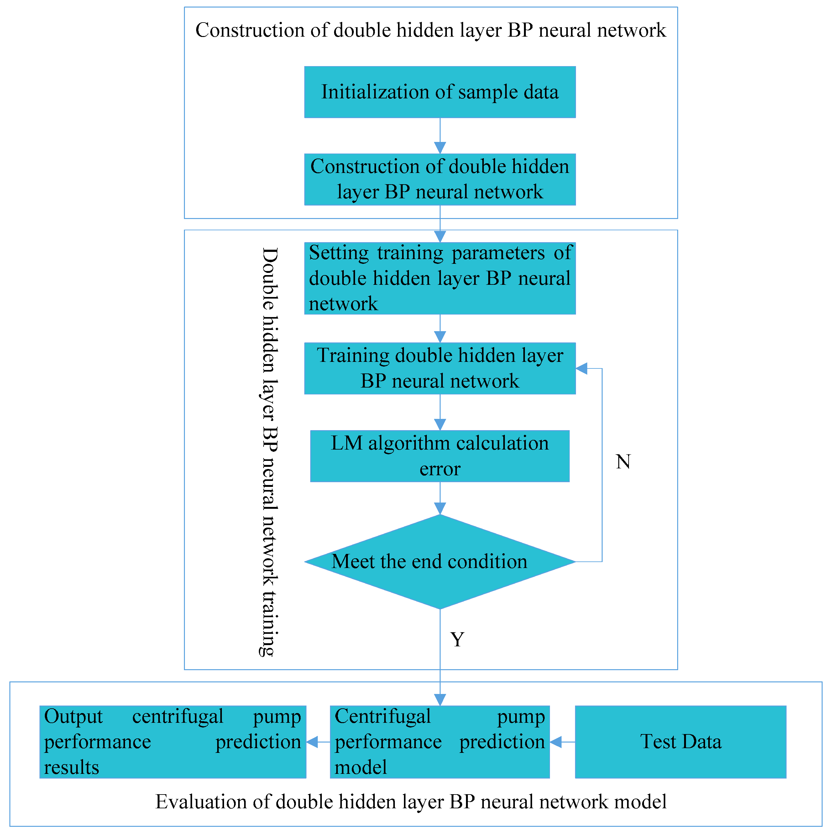
2. Structural Design of the Centrifugal Pump Performance Prediction Model

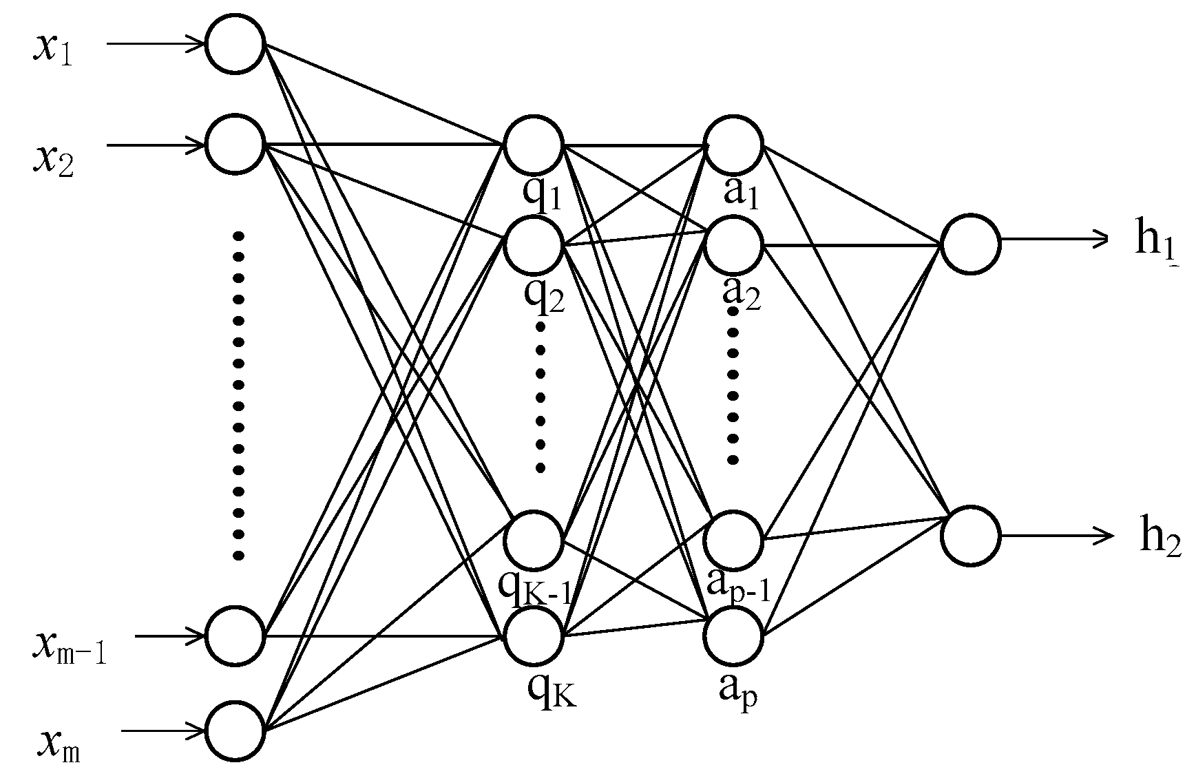
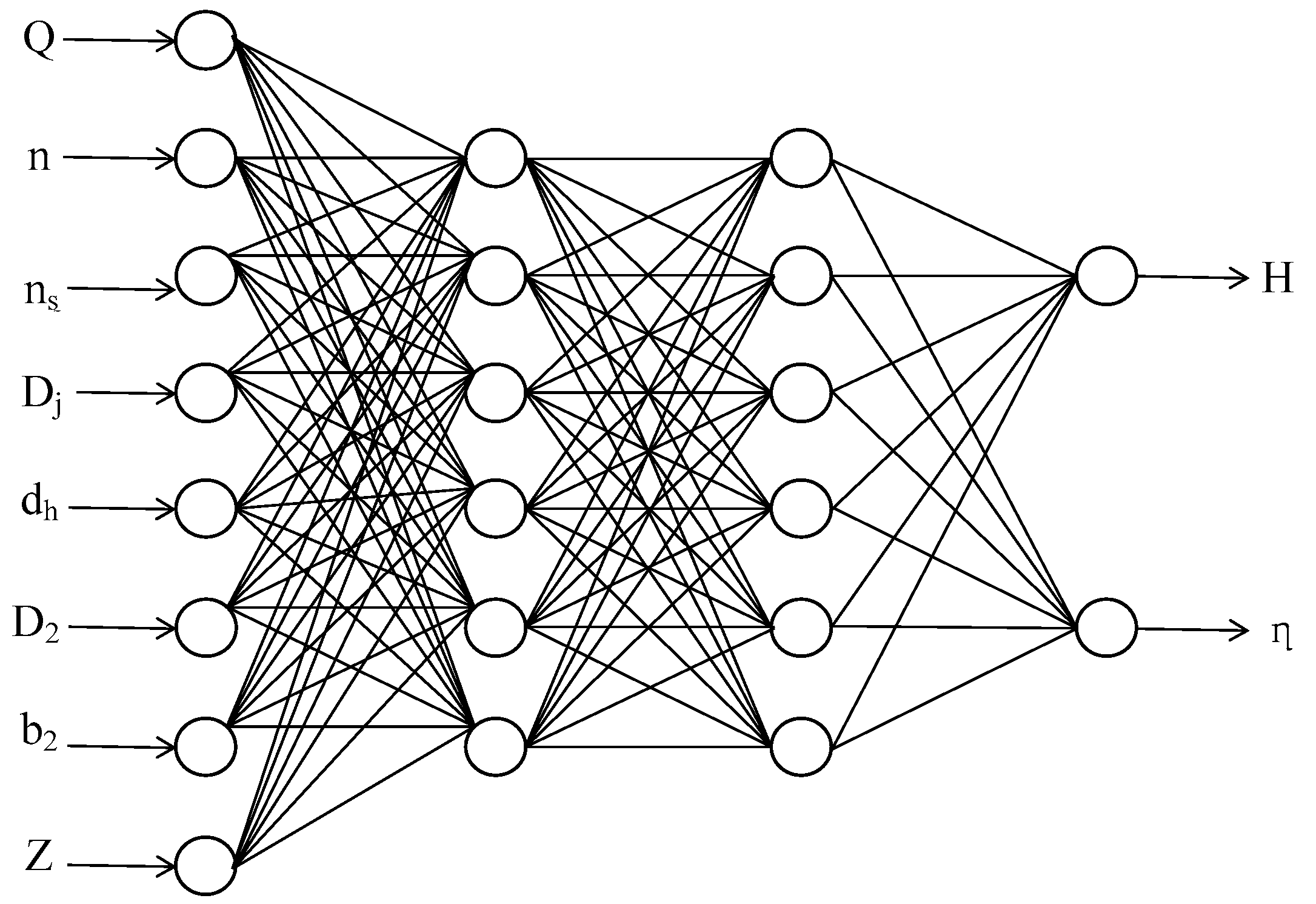
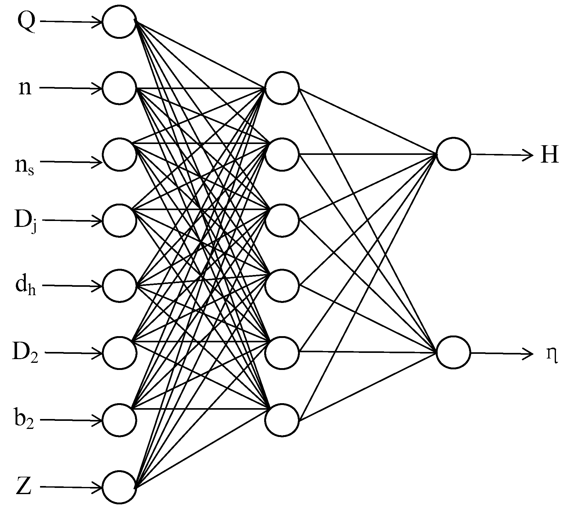
2.1. Double Hidden Layer BP Neural Network Structure

Multi-layer BP neural networks can be used to predict different engineering problems for the forward propagation of parameters and the back propagation of errors. In theory, it has the ability to approximate any nonlinear continuous map, so it is very suitable for the modeling and performance prediction of nonlinear systems [17]. In this paper, a double hidden layer BP neural network with multiple inputs and two outputs is constructed. It is assumed that the input layer is composed of m neurons, which is used to complete the input of m predicted parameters of the system. The first hidden layer is composed of k neuron nodes, which are used to complete the spatial weighted aggregation of input signals and the excitation output. The second hidden layer is composed of p neuron nodes, which are used to improve the nonlinear mapping capability of the network for a complex relationship between the input and output of the system. The output layer consists of two process neuron nodes that are used to complete the system output, as shown in Figure 1.
The transfer function of each layer in the BP neural network has a significant impact on the performance of the model. These transfer functions are usually determined experimentally. In the BP neural network, the commonly used transfer functions are linear transfer function (“purelin”), tangent transfer function (“tansig”), logarithmic sigmoid transfer function (“logsig”), etc. When the transfer function of the input layer and the first hidden layer is “tansig”, the transfer function of the first hidden layer and the second hidden layer is “tansig”, and the transfer function of the second hidden layer and the output layer is “purelin”, which are shown in the MATLAB neural network toolbox [18,19,20].
Assuming that the signal that passes from the input layer to the first hidden layer is mj, this can be expressed as in Equation (1):
m j = k = 1 m x k w kj + b j ,
where xk is the input neuron and xk represents each design parameter of the centrifugal pump in this paper. wkj represents the input layer to the first hidden layer weight and bj represents the first hidden layer bias.
The first hidden layer output signal is denoted as yj, shown as in Equation (2):
y j = tansig ( m j ) .
The signal transmitted from the first hidden layer to the second hidden layer is denoted as ni, and the calculation of ni is shown in Equation (3):
n i = j = 1 k y j w j i + b i ,
where w j i represents the weight of the first hidden layer of the second hidden layer and b i is the bias of the second hidden layer. The output signal of the second hidden layer is denoted as zi, which is expressed as in Equation (4):
z i = tansig ( n i ) .
The signals transmitted from the second hidden layer to the output layer are, respectively, recorded as s1 and s2, shown as in Equations (5) and (6):
s 1 = i = 1 p z i w i 1 + b 1 ,
s 2 = i = 1 p z i w i 2 + b 2 ,
where w i 1 and w i 2 represent the weights from the second hidden layer to the output layer, and b 1 and b 2 represent the biases of the output layer.
During the process of centrifugal pump performance prediction, the output signals of the head (H) and the efficiency (η) of the output layer are denoted as h1 and h2, respectively, which can be expressed as in Equations (7) and (8), wherein a1, a2, b1, and b2 represent the coefficients of the linear transfer function “purelin”:
h 1 = a 1 ( i = 1 p tansig ( j = 1 k tansig ( k = 1 m x k w k j + b j ) w j i + b 1 ) w i 1 + b 1 ) + b 1 ,
h 2 = a 2 ( i = 1 p tansig ( j = 1 k tansig ( k = 1 m x k w k j + b j ) w j i + b i ) w i 2 + b 2 ) + b 2 .

2.2. LM Algorithm

As the traditional gradient descent method is used to train the deep network, the convergence speed is greatly reduced because of the greater network depth. In order to solve this problem, the improved form of the Gauss-Newton method combined with the LM training algorithm is used to train the network in this paper. The proposed method can accelerate the network training and convergence speed effectively [21,22]. The LM algorithm is a second-order algorithm. So, when the gradient of the error surface is small, the LM algorithm is similar to the gradient descent method. When the gradient of the error surface is large, the LM algorithm is similar to the Gauss-Newton method [23]. In addition, the LM algorithm can estimate the learning rate (LR) in each gradient direction of the error surface according to the Hessian matrix, so compared with a first-order algorithm, the LM algorithm is more effective than others for training neural networks at present [24]. The following is a brief description of the LM algorithm: Firstly, the error index function of the neural network is set as E(x), as shown in Equation (9). Here, N is the number of samples, Yi represents the expected network output vector, Y i denotes the actual network output vector, and ri(x) represents the current error:
E ( x ) = 1 2 i = 1 N Y i Y i 2 = 1 2 i = 1 N r i 2 ( x ) .
If the weight vector of the t-th iteration of the neural network is xt, the new weight vector, xt+1, of the Newton algorithm can be obtained by Equation (10). Here, Δxt, He, and gt represent the updated value of the weight, Hessian matrix, and current gradient, respectively. He and gt can be obtained from Equations (11) and (12), where J and r(x) represent the Jacobian matrix and the error, respectively:
x t + 1 = x t + Δ x t = x t = H e t 1 g t ,
H e = J T J ,
g t = E ( x ) | x = x ( t ) = J T ( x ) r ( x ) .
However, the matrix, He, is not always reversible. In order to solve this problem, considering the introduction of a coefficient, λt, the LM algorithm after updating the weight is as shown in Equation (13), where I is an identity matrix:
x t + 1 = x t [ J T ( x t ) J ( x t ) + λ t I ] 1 J T ( x t ) r ( x t ) .
Obviously, when λt is very large, the LM algorithm approximates the gradient descent method; when λt is close to zero, it is equivalent to the Gauss-Newton algorithm. Since the approximate second-order derivative information is used in the calculation, the algorithm is much faster than the gradient descent method. In other words, the LM algorithm is superior to the Gauss-Newton method. Therefore, it is feasible to train the double hidden layer BP neural network based on the LM algorithm to improve the convergence speed of deep network training.

3. Establishment of Sample Data Sets

In the design of a centrifugal pump, the design parameters of the impeller have an important effect on the efficiency, cavitation performance, and characteristic curve of the centrifugal pump [25]. Therefore, it is necessary to investigate the influence of the design parameters of the impeller, such as flow rate (Q), rotating speed (n), impeller inlet diameter (Dj), hub diameter (dh), impeller outlet diameter (D2), specific speed (ns), blade outlet width (b2), and blade numbers (Z), on the centrifugal pump design and performance prediction. In the prediction of centrifugal pump performance, the sample data used in this paper are representative data obtained from [26], which construct 44 groups of a training sample set. These sample data are from Dalian Hongze Pump Industry, Zhejiang Institute of Mechanical, and Electrical Design, Jiangsu University Fluid Machinery Engineering Technology Research Center, China. In order to ensure the universality of the model, low, medium, and high values of ns as well as large and small values of Q are considered in the sample data. Some of these shown in Table 2.

4. Prediction Results and Analysis

The flow diagram of predicting the performance of the centrifugal pump in this paper is shown in Figure 2. It can be seen from the figure that the whole process of centrifugal pump performance prediction is divided into three parts. The first step is the construction of a double hidden layer BP neural network. In order to ensure the correctness of the training direction in the training process and accelerate the speed of the network convergence, all the data are initialized before the training starts, known as normalization processing. The normalization process here is achieved by the “prestd” function in the MATLAB toolbox. Then, the number of neurons in each hidden layer of the double hidden layer BP neural network is determined through training. The second step is the training process of the double hidden layer BP neural network. In this case, the training parameters were first set and the double-hidden BP neural network was built by MATLAB software. In the process of training, the LM algorithm was used to calculate the error value of each iteration and compare it with the set mean squared error (MSE) value. If the iterative error was less than the set value, the training would be completed; otherwise, the next iteration would continue until network convergence was achieved. The third step is the evaluation of the double hidden layer BP neural network model. From the second step, the centrifugal pump back propagation (CPBP) performance prediction model will be established, then the test data will be input into this model for the prediction of the head and efficiency.

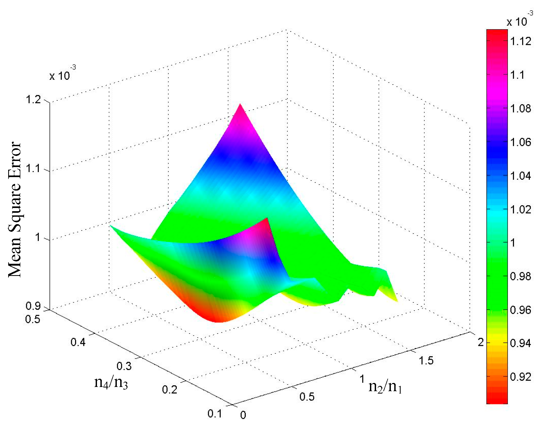
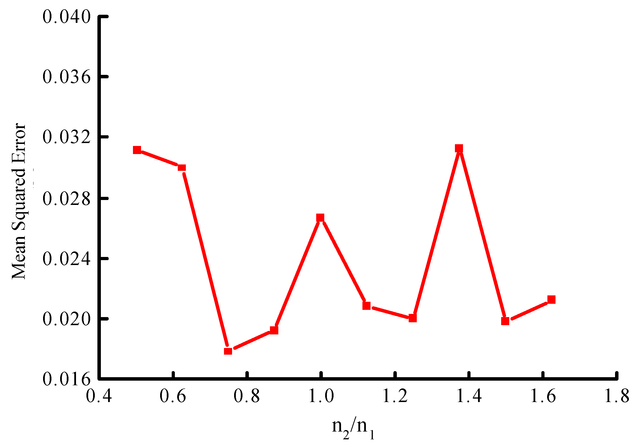
4.1. Parameter Selection of the CPBP Model

With the aim of overcoming the shortcomings of predicting the performance of a centrifugal pump with a single hidden layer BP neural network, a double hidden layer BP neural network was constructed in this paper, including one input layer, two hidden layers, and one output layer. In order to obtain a better nonlinear mapping relationship of the related parameters through network learning, the S-type tangent function and linear function were used for the transfer functions of the two hidden layers and the output layer, respectively. Similar to the traditional BP neural network, the performance of the double hidden layer BP neural network is also affected by the number of neurons in the input layer and hidden layer. In general, the number of input layer neurons is determined by the number of input sample variables. So, the number of neurons in the input layer was set as eight in this paper. Similarly, the number of neurons in the output layer needs to be equal to the number of the predicted parameters. The number of neurons in the output layer of the network was set as two, including the head and efficiency of the centrifugal pump. With regard to the determination of the number of neurons in the hidden layer, this paper adopted the design method of the number of neurons in the hidden layer [27,28], as shown in Equation (14):
c = d + u + f ,
where c, d, and u represent the number of neurons in the hidden layer, input layer, and output layer, respectively. The values of the constant “f” ranged from 1 to 10, so the range of neuron numbers in the hidden layer was 4 to 13.
The number of hidden layer neurons is input into the corresponding model and then the network is trained once again. Figure 3 shows the MSE values corresponding to different networks. The horizontal axis is the ratio (n2/n1) of the number of neurons (n2) in the first hidden layer to the number of neurons (n1) in the input layer; the longitudinal axis is the ratio (n4/n3) of the number of neurons (n4) in the output layer to the number of neurons (n3) in the second hidden layer; and the vertical axis is the training MSE corresponding to each network. As the numbers of neurons in the first hidden layer and the second hidden layer were both six, the corresponding MSE was the minimum. Therefore, the final structure of the double hidden layer BP neural network suitable for the prediction of centrifugal pump performance was 8-6-6-2. Figure 4 is the structure diagram of the CPBP network.

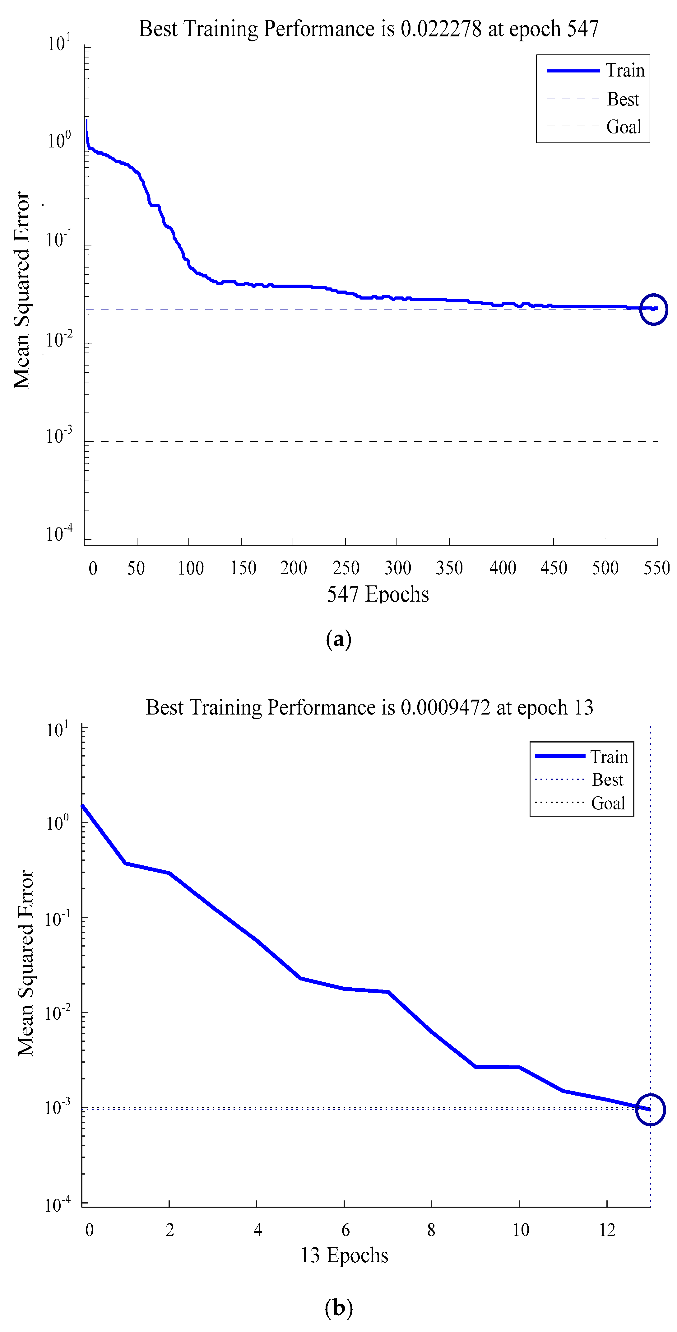
4.2. Training Process of CPBP Model

The training parameters of neural networks have an important influence on the performance prediction of centrifugal pumps, so it is necessary to choose the appropriate training parameters. The parameters used in the CPBP network training include the maximum number of iterations: Epochs, LR, momentum factor (MF), and MSE. These training parameters have a direct impact on the prediction accuracy of the final centrifugal pump performance. The CPBP network model can be established with the help of the neural network toolbox in MATLAB to determine the design values of the network training parameters, as shown in Table 3.
The training network is started after the CPBP network is built. During the training process, the back propagation of error is used to iterate repeatedly until the convergence of the CPBP network is achieved. Finally, the prediction model of the centrifugal pump can be established by the CPBP network.

4.3. Prediction Results of CPBP Model

In order to verify the accuracy of the prediction method, five sets of test data provided by Shanghai Kaiquan Pump Co., Ltd. China, were input into the trained model to obtain the prediction values of the head and efficiency. The corresponding relative error can be calculated between the experimental and the predictive values. Simultaneously, the prediction accuracy of the CPBP network model can be obtained. The comparison between the experimental and the predicted results is shown in Table 4. Among them, H** and η** are the head and efficiency predicted by the CPBP model, respectively.
The maximum relative error of the head predicted by the CPBP model compared with the experimental results was 11.87%, the minimum was 0.13%, and the average relative error was 4.35%. From these error values, it can be found that the error distribution was relatively average. The maximum relative error between the model prediction and the experimental efficiency was 4.99%, the minimum was 0.47%, and the average relative error was 2.94%, so the error distribution was also uniform. The average relative error of the prediction values on the head and efficiency indicate the reliability of the CPBP model.

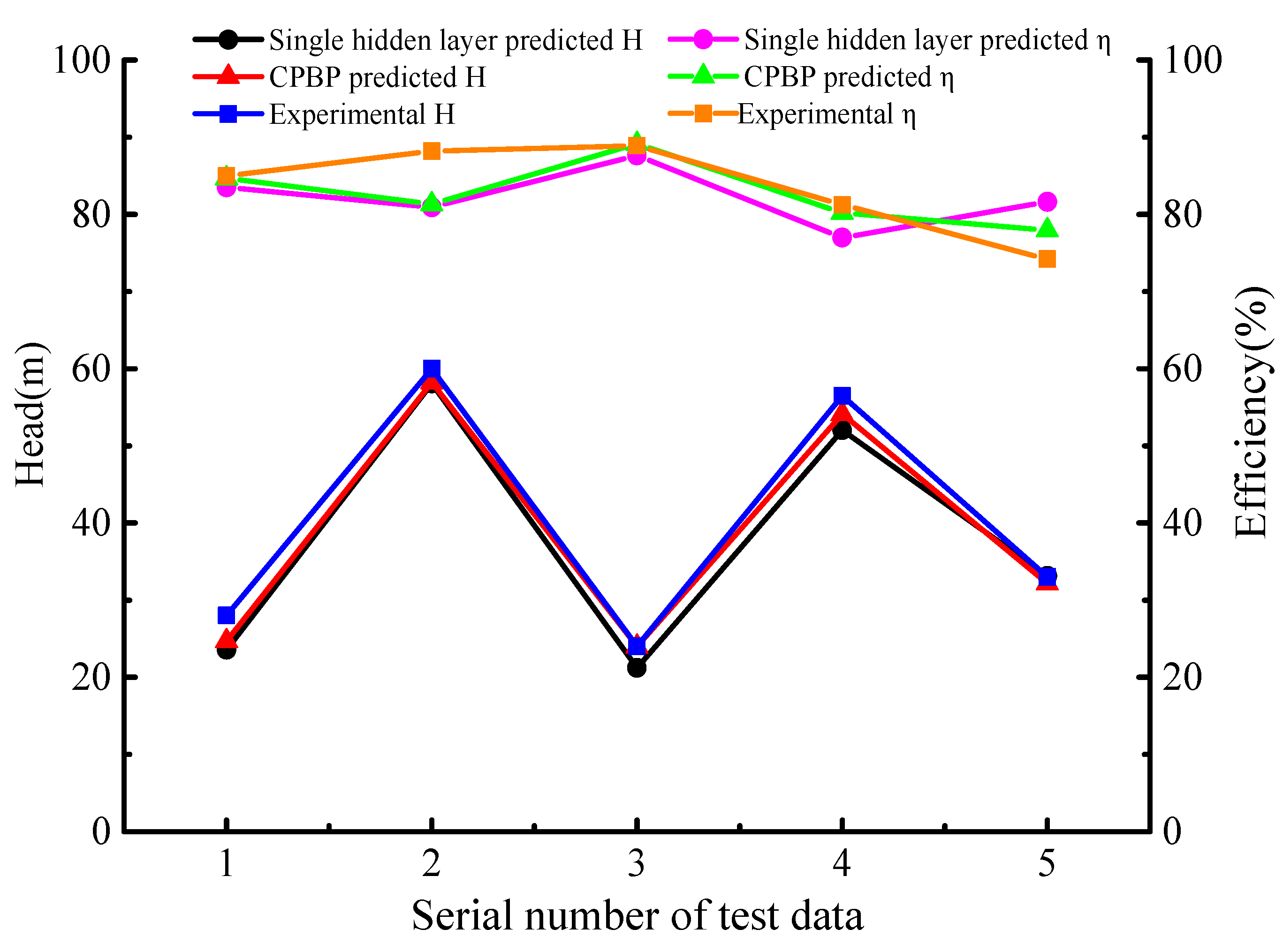
4.4. Comparison of Results

In order to compare the prediction accuracy of the CPBP network with the traditional single hidden layer BP neural network, the traditional single hidden layer BP neural network with the best prediction effect was constructed to predict the performance of the centrifugal pump. Firstly, Equation (14) was used to determine the value range of the number of hidden layer neurons when the number of input neurons was eight and the number of output neurons was two. After calculation, the value range of hidden layer neurons was also 4 to 13. Then, the single hidden layer BP networks corresponding to 4 to 13 hidden layer neurons were set up in MATLAB and trained. The MSE values corresponding to different networks are shown in Figure 5, where the abscissa is the ratio (n2/n1) of the number of neurons (n2) in the hidden layer to the number of neurons (n1) in the input layer and the ordinate is the training MSE corresponding to each network.
As can be seen from Figure 5, when the number of neurons in the hidden layer was six, the corresponding MSE was the smallest. That is, the single hidden layer BP neural network composed of six neurons in the hidden layer had the best prediction effect compared with other single hidden layer BP neural networks. Its structure is shown in Figure 6.
Five groups of identical test data with the CPBP were input into the centrifugal pump prediction model obtained by the single hidden layer BP neural network training to obtain the predicted results. The results of the prediction of centrifugal pump performance between the single hidden layer BP network and the double hidden layer BP network were compared, as is shown in Table 5 and Figure 7. Among them, H* and η* are the head and efficiency of the single hidden layer BP neural network prediction, respectively. Δη* and △H* are the relative errors of the efficiency and head of the single hidden layer BP neural network, respectively. Δη** and △H** are the relative errors of the efficiency and head of the CPBP model, respectively. Compared with the CPBP network, the maximum, the minimum, and the average relative error of the head value of the single hidden layer BP network increased by 11.41%, 0.23%, and 3.40%, respectively. Meanwhile, the maximum, the minimum, and the average relative error of the efficiency prediction value increased by 4.99%, 0.47%, and 2.37%, respectively. It can be concluded that the CPBP network has a higher prediction accuracy than the single hidden layer BP network for the performance prediction of centrifugal pumps.
As can be seen from Figure 7, the predicted and the experimental values exhibited the same change trend; the small deviation may be caused by the accuracy of the experimental data and the deficiencies of the training samples.
Figure 8 shows the variation of the MSE during the training of the BP network with a single hidden layer and the CPBP network. It can be seen that the traditional single hidden layer BP network had difficulty in achieving a high convergence accuracy quickly compared with the CPBP network. Therefore, the CPBP network is more effective in predicting the performance of centrifugal pumps compared to the traditional single hidden layer BP neural network.

5. Conclusions

(i) In this paper, a new CPBP model for the performance prediction of centrifugal pumps based on design and structure parameters was established. The LM algorithm was used to accelerate the convergence rate of the double hidden layer BP network. The proposed model improves the mapping ability of the complex relationship between the input and output of the nonlinear system, known as the centrifugal pump performance, with its structure and operation parameters.
(ii) The CPBP network could easily achieve a high convergence accuracy quickly compared with the traditional single hidden layer BP network.
(iii) Compared with the traditional single hidden layer BP network, the average relative error of the head and efficiency prediction values of the CPBP network decreased by 3.40% and 2.37%, respectively, and the training time of CPBP model was only 1/42 of that of the traditional BP network. This indicates that the CPBP network model is more suitable for the rapid and efficient determination of the optimum design of a centrifugal pump.

Author Contributions

W.H. conceived and designed the research, L.N. drafted the article, M.S. completed the neural network architecture and verification, Y.C. collected and collated the test sample data, R.L. is the leader of the research team. X.Z. completed the English check.

Funding

This study was supported by the National Key R&D Program Projects of China (Grant no. 2018YFB0606100) and the National Natural Science Foundation of China (Grant no. 51669012, 51579125).

Acknowledgments

The authors would like to acknowledge the support in the form of experimental data provided by Shanghai Kaiquan Pump Co., Ltd. China.

Conflicts of Interest

There are no known conflicts of interest.

References

  1. Kaewnai, S.; Chamaoot, M.; Wongwises, S. Predicting performance of radial flow type impeller of centrifugal pump using CFD. J. Mech. Sci. Technol. 2009, 23, 1620–1627. [Google Scholar] [CrossRef]
  2. Ran, J. Research and Implementation of Performance Prediction of Centrifugal Pump Based on Neural Network; University of Electronic Science and Technology of China: Chengdu, China, 2014. [Google Scholar]
  3. Li, D.J.; Li, Y.Y.; Li, J.X. Gesture Recognition Based on BP Neural Network Improved by Chaotic Genetic Algorithm. Int. J. Autom. Comput. 2018, 15, 21–30. [Google Scholar] [CrossRef]
  4. Peng, Z.Q.; Cao, C.; Huang, J.Y. Seismic signal recognition using improved BP neural network and combined feature extraction method. J. Cent. South Univ. 2014, 21, 1898–1906. [Google Scholar] [CrossRef]
  5. Nie, S.B.; Guan, X.F.; Liu, H.L. Exploration of Predicting the Performance of Centrifugal Pumps by Artificial Neural Network. Pump Technol. 2002, 5, 16–18. [Google Scholar]
  6. Yao, Y.F.; Jiang, Q.Y.; He, R.G. Performance Prediction of Centrifugal Pump Based on BP Neural Network. Mech. Des. Manuf. 2008, 10, 73–74. [Google Scholar]
  7. Cong, X.Q.; Yuan, S.Q.; Yuan, D.Q. Performance Prediction of Centrifugal Pump Based on Improved BP Neural Network. J. Agric. Mach. 2006, 37, 56–59. [Google Scholar]
  8. Jiang, W.Z.; Duan, S.Q.; Yang, C.M. Optimization design of centrifugal pump impeller based on CFD simulation and BP neural network. Mach. Tool Hydraul. 2016, 44, 67–70. [Google Scholar]
  9. Zayani, R.; Bouallegue, R.; Roviras, D. Adaptive Predistortions Based on Neural Networks Associated with Levenberg-Marquardt Algorithm for Satellite Down Links. EURASIP J. Wirel. Commun. Netw. 2008, 2008, 132729. [Google Scholar] [CrossRef] [Green Version]
  10. Camargo, A.; He, Q.; Palaniappan, K. Performance evaluation of optimization methods for super-resolution mosaicking on UAS surveillance videos. In Proceedings of the SPIE Defense, Security, and Sensing 2012, Baltimore, MD, USA, 24–26 April 2012; Volume 8355, p. 30. [Google Scholar]
  11. Jebur, A.A.; Atherton, W.; AlKhaddar, R.M. Settlement Prediction of Model Piles Embedded in Sandy Soil Using the Levenberg–Marquardt (LM) Training Algorithm. Geotech. Geol. Eng. 2018, 36, 2893–2906. [Google Scholar] [CrossRef]
  12. Comon, P.; Luciani, X.; De Almeida, A.L.F. Tensor decompositions, alternating least squares and other tales. J. Chemom. Soc. 2010, 23, 393–405. [Google Scholar] [CrossRef]
  13. Wang, T.Y. Research and Implementation of LM-BP Neural Network Intrusion Detection System; Hunan University: Changsha, China, 2007. [Google Scholar]
  14. Zhao, H.; Zhou, R.X. Neural Network Supervisory Control Based on Levenberg-Marquardt Algorithm. J. Xi’an Jiaotong Univ. 2002, 36, 523–527. [Google Scholar]
  15. Song, Z.J.; Wang, J. Fuzzy clustering and LM algorithm to improve BP neural network for transformer fault diagnosis. High. Volt. Electr. Appl. 2013, 5, 54–59. [Google Scholar]
  16. Cui, D.W. Comprehensive evaluation of water resources vulnerability in Wenshan Prefecture of Yunnan Province based on improved BP neural network model. J. Yangtze River Sci. Res. Inst. 2013, 30, 1–7. [Google Scholar]
  17. Ding, H.; Dong, W.Y.; Wu, D.M. Water Level Prediction of Double Hidden Layer BP Neural Network Based on LM Algorithm. Stat. Decis. 2014, 5, 16–19. [Google Scholar]
  18. Khayet, M.; Cojocaru, C. Artificial neural network model for desalination by sweeping gas membrane distillation. Desalination 2013, 308, 102–110. [Google Scholar] [CrossRef] [Green Version]
  19. Choi, H.K.Y.; Lin, W.; Loon, S.C. Facial Scanning with a Digital Camera: A Novel Way of Screening for Primary Angle Closure. J. Glaucoma 2015, 24, 522–526. [Google Scholar] [CrossRef] [PubMed]
  20. Cai, Z.L.; Chen, X.L.; Shi, W.R. Improvement of Comprehensive Evaluation Method of Learning Effect Based on BP Neural Network. J. Chongqing Univ. 2007, 30, 96–99. [Google Scholar]
  21. Gao, J.; Zhang, Y.; Du, Y. Optimization of the tire ice traction using combined Levenberg–Marquardt (LM) algorithm and neural network. J. Braz. Soc. Mech. Sci. Eng. 2019, 41, 40. [Google Scholar] [CrossRef]
  22. An, R.; Li, W.J.; Han, H.G. An improved Levenberg-Marquardt algorithm with adaptive learning rate for RBF neural network. In Proceedings of the 2016 35th Chinese Control Conference (CCC), Chengdu, China, 27–29 July 2016. [Google Scholar]
  23. Zhang, H.H.; Tao, Y.R.; Hu, J. Prediction model of photosynthetic rate of cucumber seedlings fused with chlorophyll content. J. Agric. Mach. 2015, 46, 259–263. [Google Scholar]
  24. Wilamowski, B.M.; Yu, H. Improved Computation for Levenberg–Marquardt Training. IEEE Trans. Neural Netw. 2010, 21, 930–937. [Google Scholar] [CrossRef] [PubMed]
  25. Wang, Y.Y. Effect of Blade Wrap Angle and Exit Angle on Impeller Performance; Lanzhou University of Technology: Lanzhou, China, 2017. [Google Scholar]
  26. Guan, X.F. Modern Pump Theory and Design; China Aerospace Publishing House: Beijing, China, 2010. [Google Scholar]
  27. Jiao, B.; Ye, M.X. Method for determining the number of hidden layer units in BP neural network. J. Shanghai Dianji Univ. 2013, 16, 113–116. [Google Scholar]
  28. Wang, R.B.; Xu, H.Y.; Li, B. Research on the Method of Determining the Number of Nodes in BP Neural Network. Comput. Technol. Dev. 2018, 28, 31–35. [Google Scholar]
Figure 1. Double hidden layer back propagation (BP) neural network structure.
Energies 12 02709 g001
Figure 2. Centrifugal pump performance prediction flow diagram with the centrifugal pump back propagation (CPBP) model.
Energies 12 02709 g002
Figure 3. Comparison of mean squared errors of back propagation (BP) networks with different double hidden layers.
Energies 12 02709 g003
Figure 4. Centrifugal pump back propagation (CPBP) neural network structure diagram.
Energies 12 02709 g004
Figure 5. Comparison of the mean squared errors of different single hidden layer back propagation (BP) networks.
Energies 12 02709 g005
Figure 6. Single hidden layer back propagation (BP) network structure diagram.
Energies 12 02709 g006
Figure 7. Comparison between the prediction results and experimental results of five test sets.
Energies 12 02709 g007
Figure 8. Change of the mean squared errors on the back propagation (BP) neural network with different hidden layers. (a) Back propagation (BP) network with a single hidden layer; (b) centrifugal pump back propagation (CPBP) network.
Energies 12 02709 g008
Table 1. Disc loss with different specific speeds of a centrifugal pump.
Specific Speed30405060708090100150200
Disc Loss/%28.520.415.712.710.69.17.97.04.43.1
Table 2. Centrifugal pump performance prediction model sample data.
Serial NumbernsQ (m3/h)N (r/min)Dj (mm)dh (mm)D2 (mm)b2 (mm)ZH (m) η (%)
123.112.529005202424480.7842.21
23021290060024510108041
33312.529004802006550.3451.09
447.212.529004401605.6531.2556.32
54830014501754554717710075
658752950100502901168070
7731482900110252781569080.5
8811401450138323171963079.7
9902002900110252551878480
101031301450140382622362182
11131400145019003453563283
121512431450162352623461986.8
132052600740450064012052588.9
142256300490700096518652388
1530266506606250775.518742485.8
Table 3. Training parameter settings.
ParameterEpochsLRMFMSE
Setting5500.040.950.001
Table 4. Comparison of prediction results and experimental results of five test sets.
Serial NumberInput ValueExperimental ValuePredictive Value
nsQ (m3/h)n (r/min) Dj (mm)dh (mm)D2 (mm)b2 (mm)ZH (m)H (%)H** (m)η** (%)
1180620145022550340545288524.675684.6602
21147751450240484404266088.258.223381.3399
32463500740500065013752488.923.967289.1542
485.6100290090021016656.581.2554.109580.2150
5128.1100290010001781763374.232.148477.9264
Table 5. Comparison of the results of centrifugal pump performance prediction between the single hidden layer back propagation (BP) network and the double hidden layer back propagation (BP) network.
Serial NumberExperimental ValuePredicted Value and Relative Error of BP Network with Single Hidden LayerPredicted Value and Relative Error of Double Hidden Layer (CPBP Model)
H/mη/%H*/mη*/%△η*/%△H*/%H**/mη**/%△η**%△H**/%
1288523.570083.51831.740015.820024.675684.66020.399011.8700
26088.258.087380.93518.24003.188058.223381.33997.77002.9600
32488.921.227587.64471.400011.550023.967289.15420.28600.1360
456.581.2552.017976.99555.24007.900054.109580.21501.27004.2300
53374.233.112781.61549.99000.340032.148477.92645.00002.5800

