Pressure Transient Performance for a Horizontal Well Intercepted by Multiple Reorientation Fractures in a Tight Reservoir

 ,
, 
Abstract
:
1. Introduction
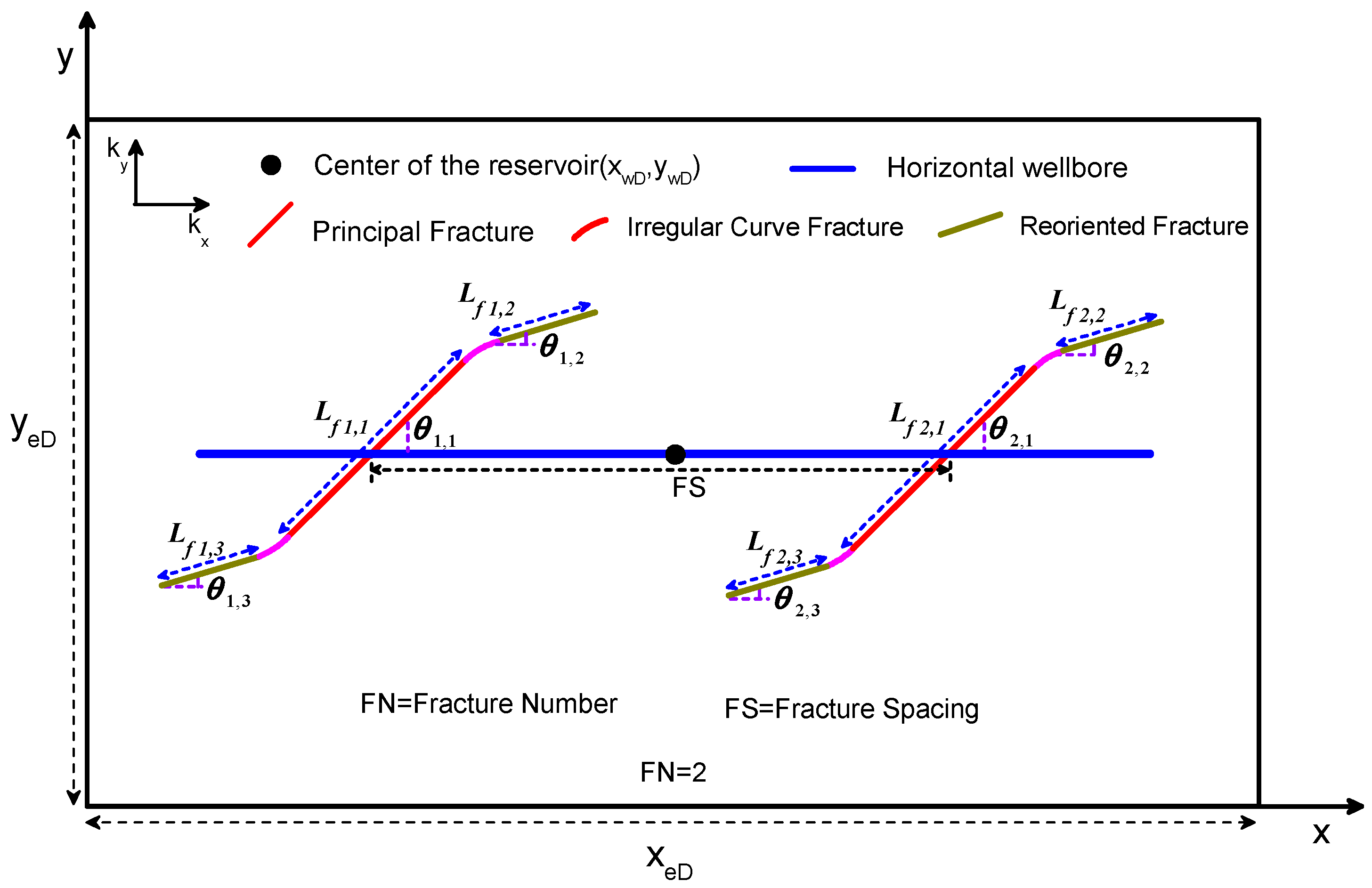
2. Physical Model
- (1)
- The tight reservoir is rectangular in shape. Single-phase Darcy flow occurs in the anisotropic tight reservoir. The permeability of the reservoir in the x- and y-direction is kx and ky, respectively.
- (2)
- The horizontal well is fully intercepted by arbitrary reorientation fractures with constant height and width. The horizontal wellbore is deployed parallel to the x-axis, and all fractures’ height is equal to the reservoir thickness.
- (3)
- Fluid in the horizontal wellbore and reservoir is constant viscosity and slightly compressible, and flow rates from each reorientation fracture contribute to the horizontal well total rate, although they may change over time. The horizontal wellbore is infinite-conductivity and no pressure loss occurs along the wellbore.
- (4)
- This reservoir is fully penetrated by all reorientation fractures. For the i-th reorientation fracture, its principal fracture angle is θi,1, and its reoriented fractures angles are θi,2 and θi,3, respectively. All reorientation fractures have a finite conductivity and their tips are assumed to be impermeable boundaries.
- (5)
- Gravity effect is negligible, as well as the influence of the temperature on different reservoir parameters.
3. Mathematical Models
3.1. Dimensionless Definitions
3.2. Reservoir Flow Model
3.3. Reorientation Fracture Flow Model
3.4. Semi-Analytical Solutions
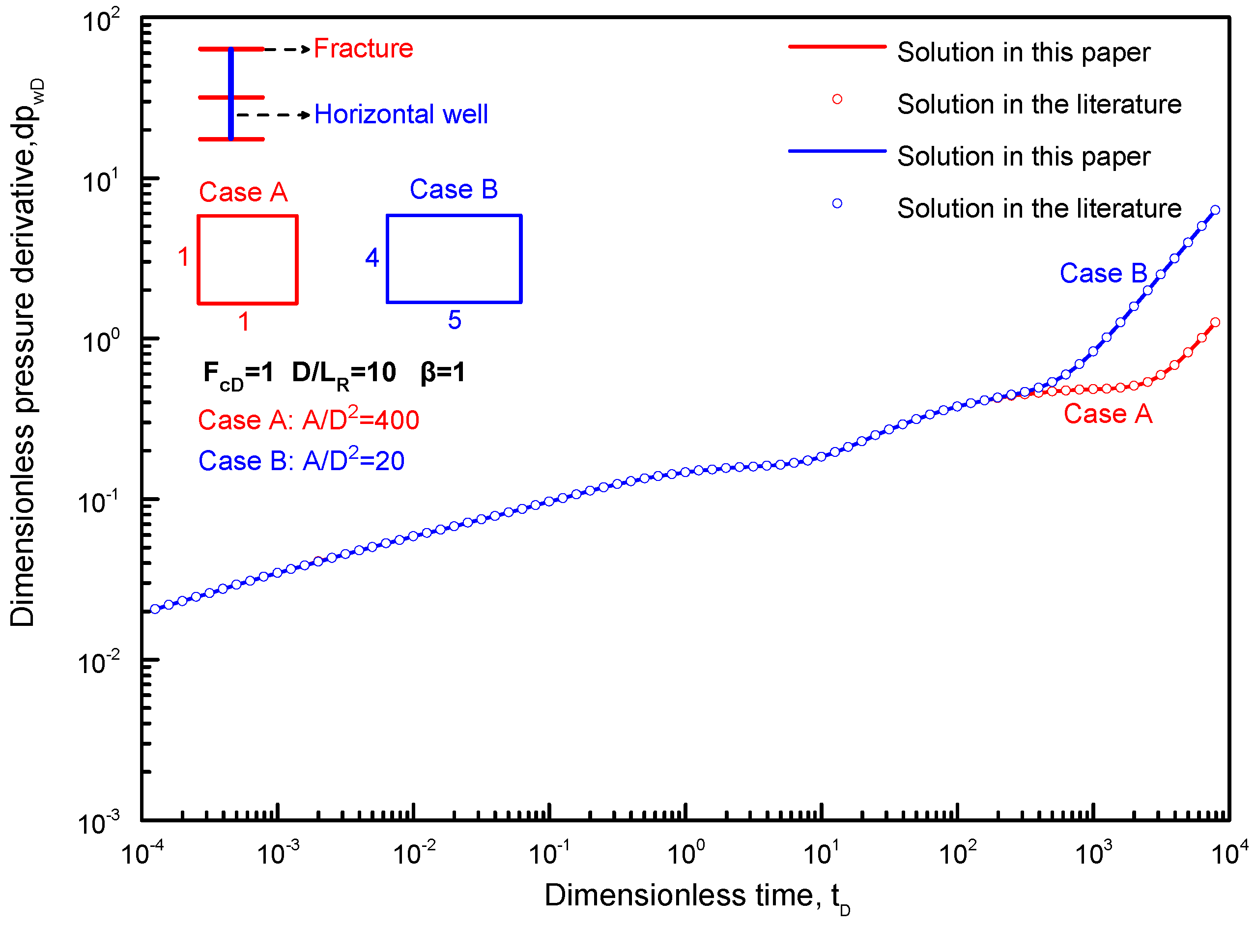
4. Verification and Comparison
5. Results and Discussion
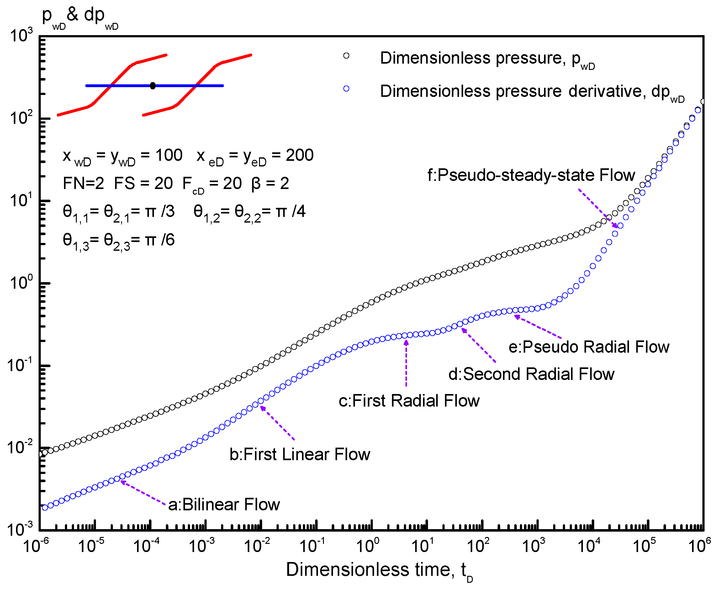
5.1. Transient Flow Characteristics
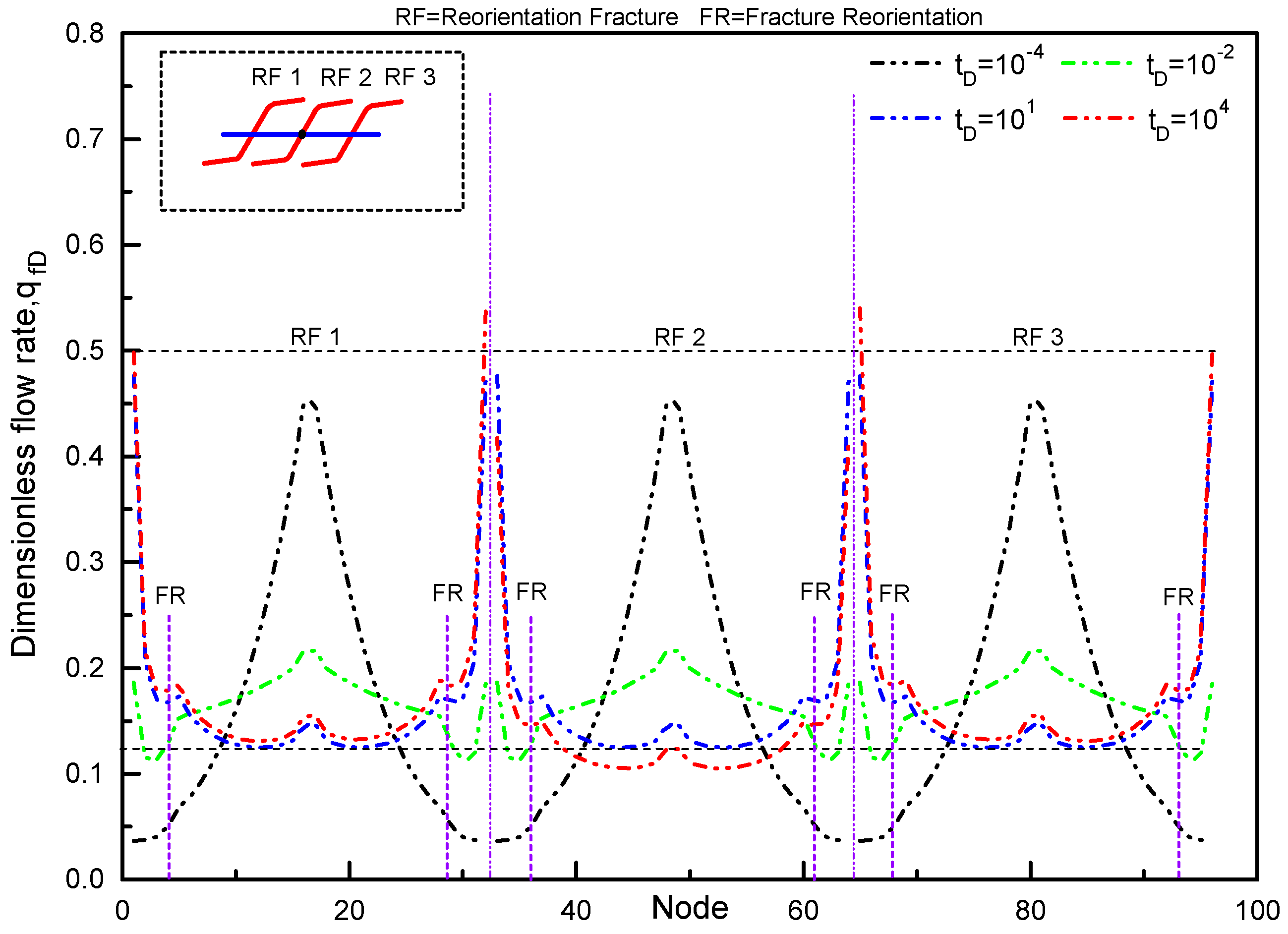
5.2. Production Rate Distribution
5.3. Parameter Influence on Transient Pressure Behavior
5.3.1. Effect of Principal Fracture Angle (PFA) on Type Curves
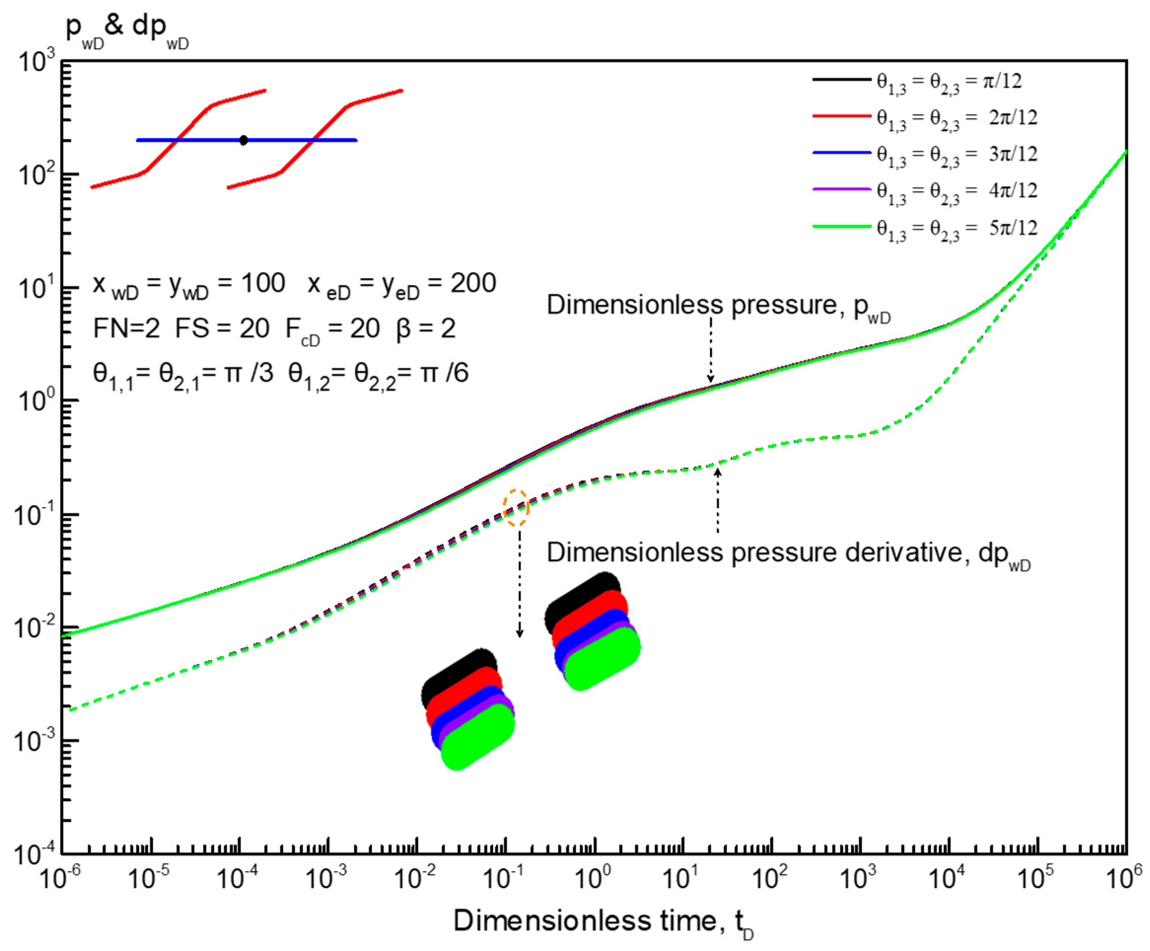
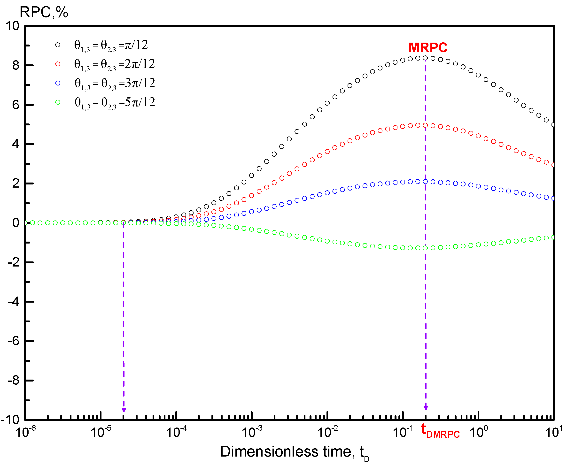
5.3.2. The effect of reoriented fracture angle (RFA) on type curves
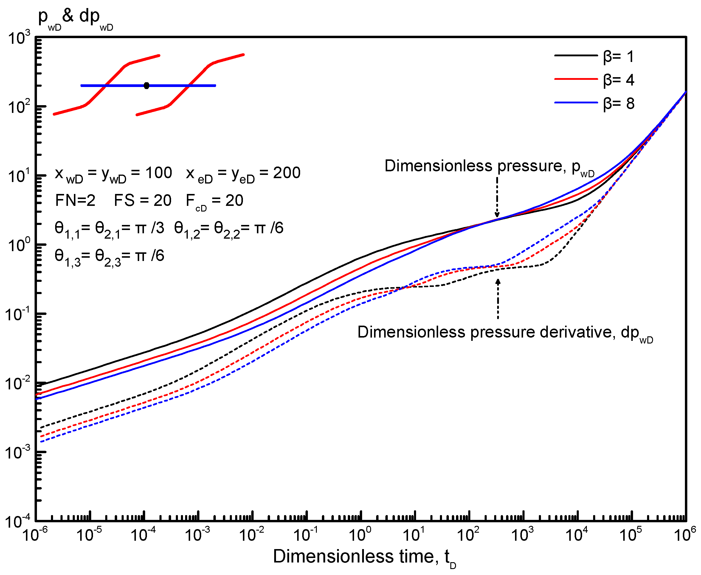
5.3.3. Effect of Permeability Anisotropy on Type Curves
5.3.4. Effect of Fracture Conductivity on Type Curves
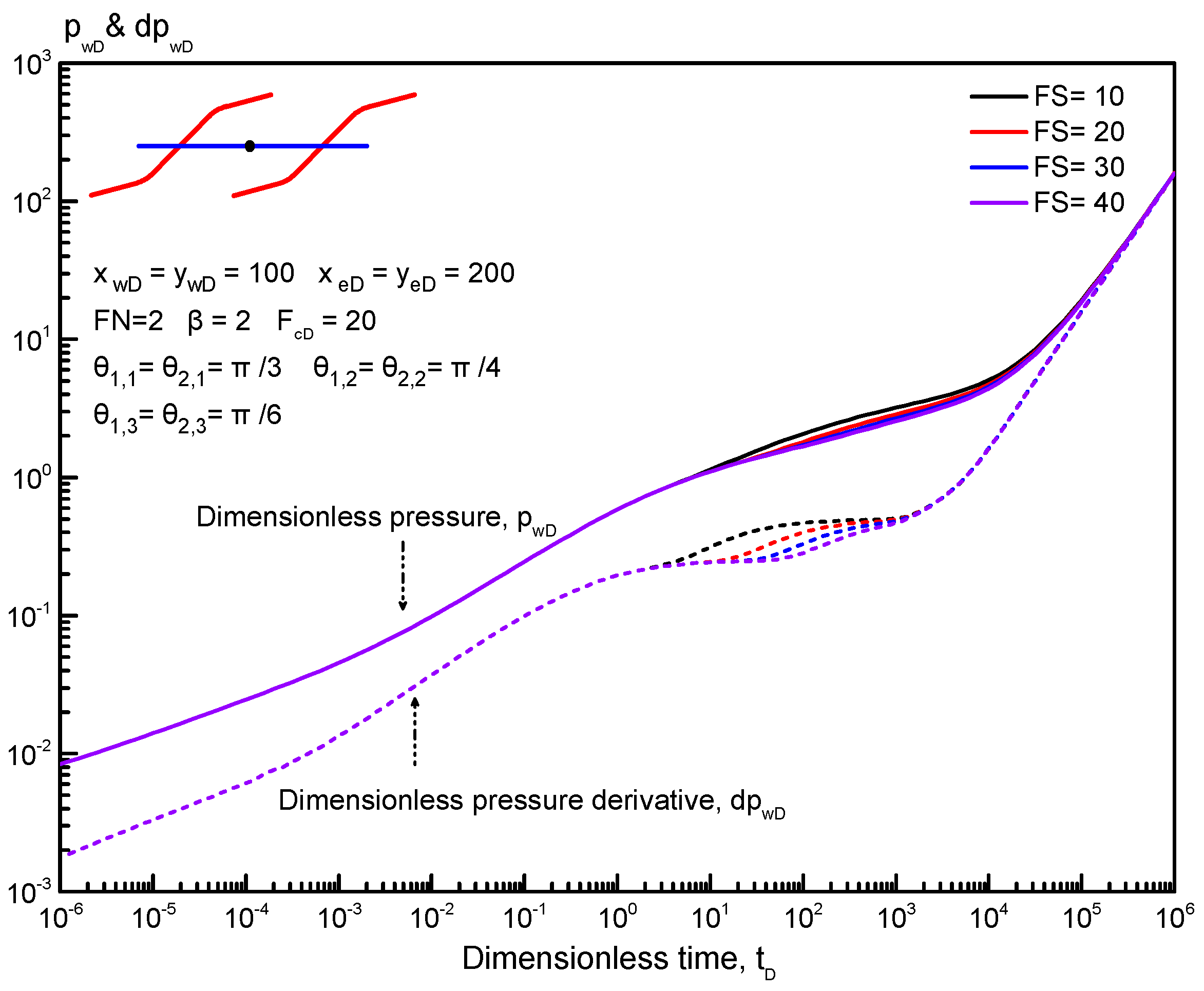
5.3.5. Effect of Dimensionless Fracture Spacing (FS) on Type Curves
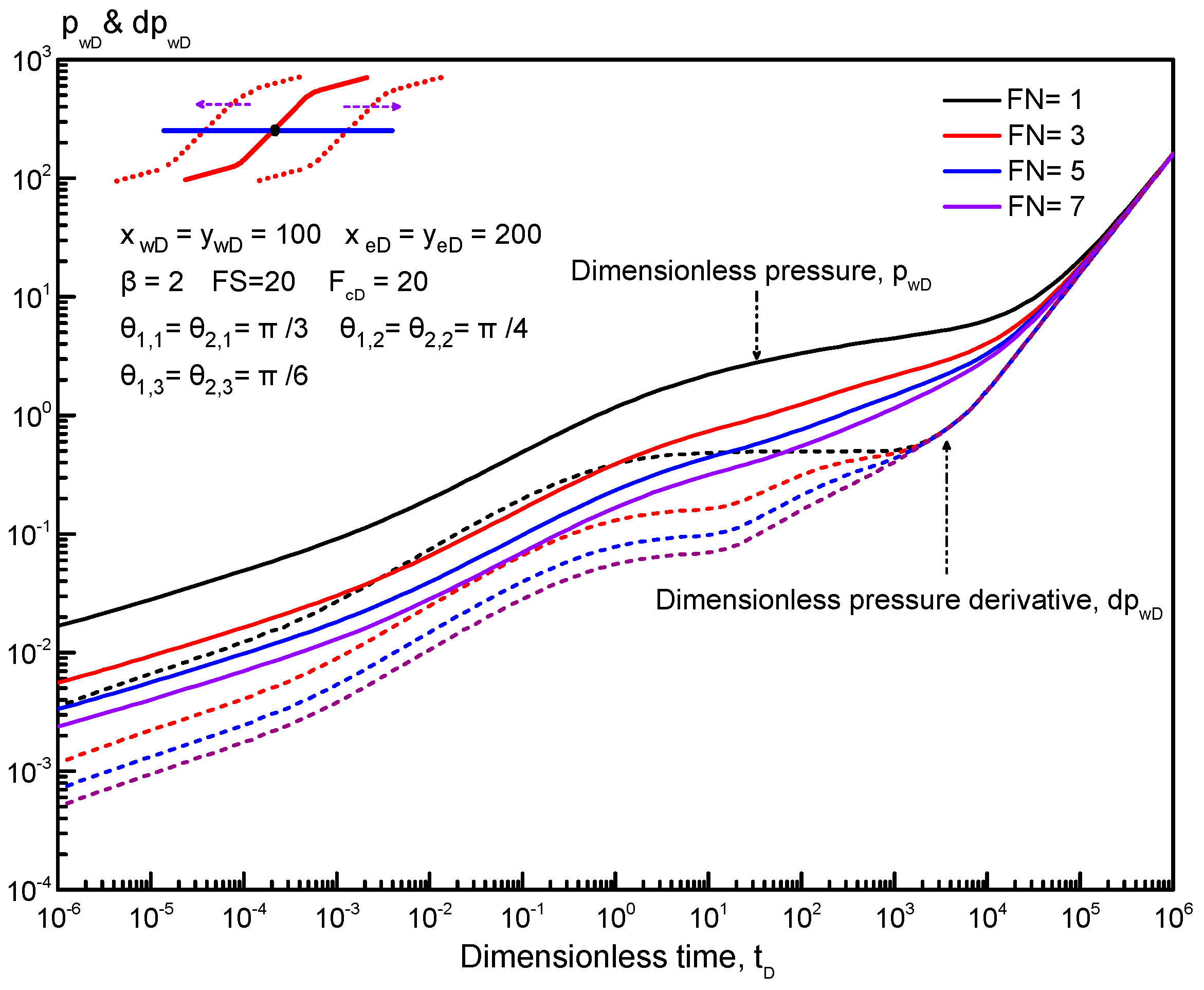
5.3.6. Effect of Fracture Number (FN) on Type Curves
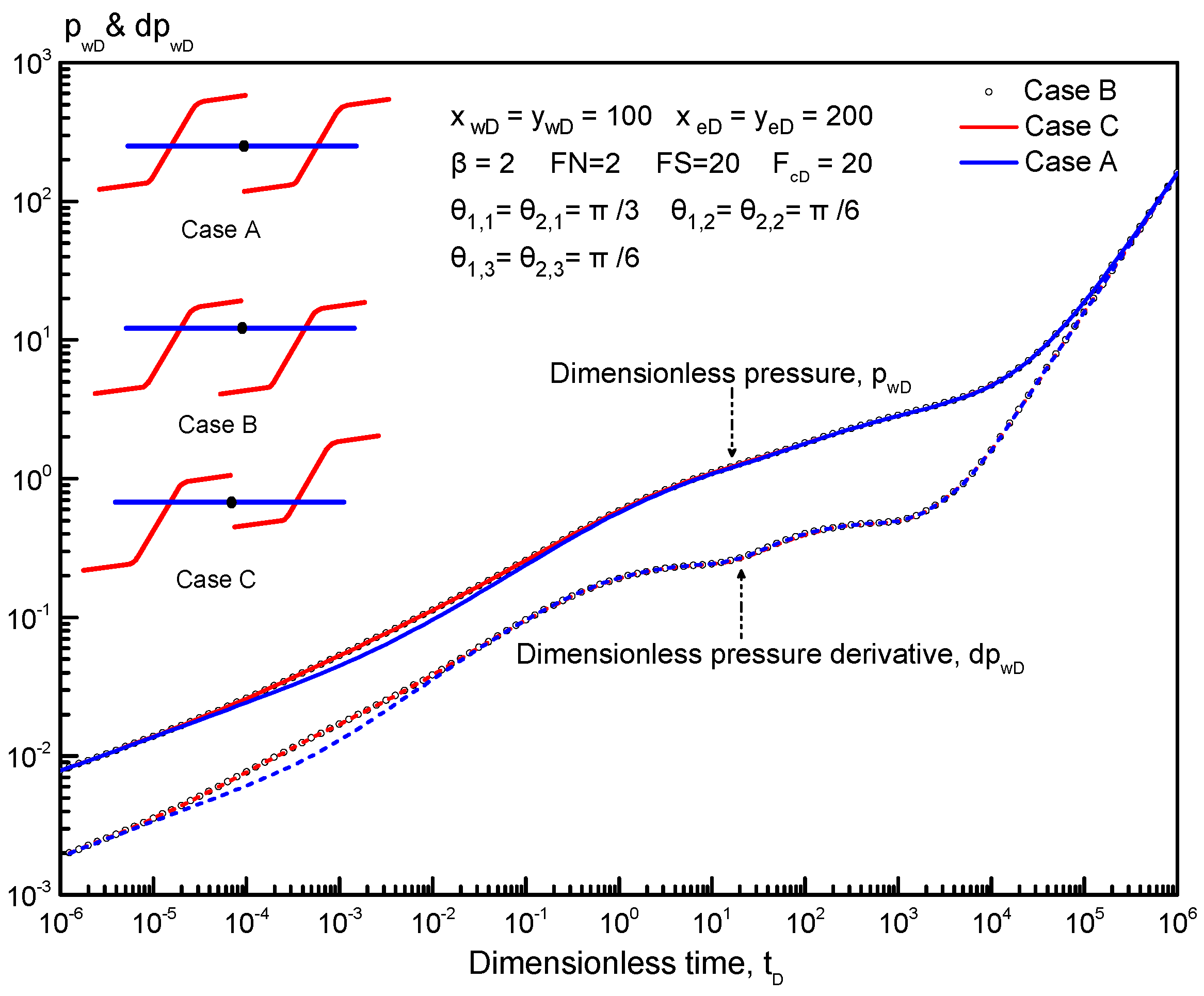
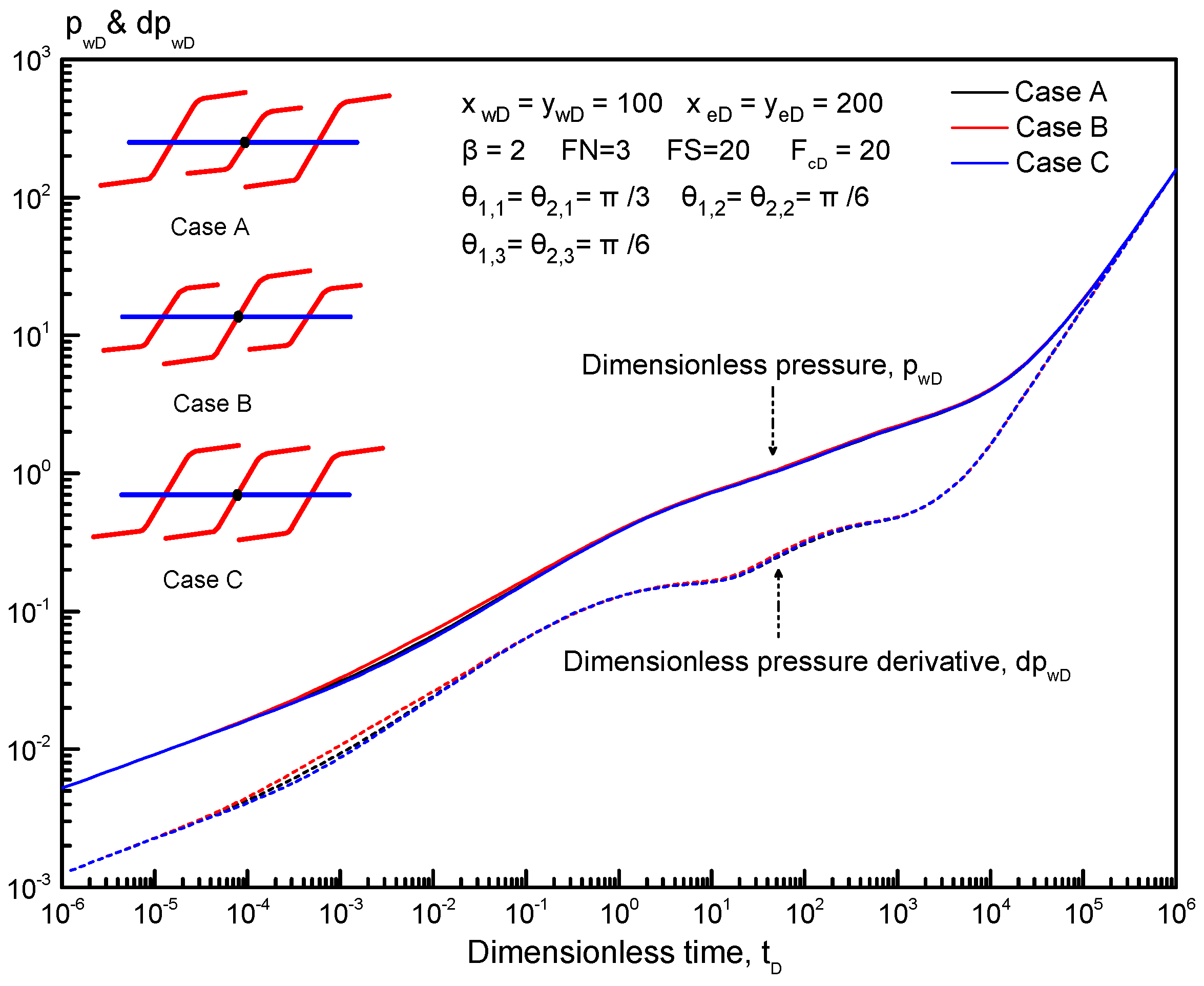
5.3.7. Effect of Complex Fracture Configuration on Type Curves
6. Conclusions
- (1)
- For a horizontal well perforated by multiple reorientation fractures with finite-conductivity in an anisotropic rectangular reservoir, six typical flow regimes can be found on type curves, including bilinear flow regime, first linear flow regime, first radial flow regime, second radial flow regime, pseudo-radial flow regime, and pseudo-steady-state flow regime. Meanwhile, the occurrence and duration of these typical regimes are determined by some significant parameters, such as the permeability anisotropic factor, fracture reorientation, fracture spacing, fracture number, and fracture configuration.
- (2)
- Fracture reorientation has an obvious effect on the production rate distribution along the fracture extension, particularly in the anisotropic tight reservoir. The production rate distribution curves for a horizontal well with three reorientation fractures in an anisotropic tight reservoir oscillate, and the outermost reorientation fracture has a larger production rate than the inner reorientation fracture due to a larger contact area with the reservoir.
- (3)
- Fracture reorientation is one of the highlights of this work. For an anisotropic tight reservoir, the horizontal well should be deployed parallel to the direction of the principal permeability axis, and all reoriented fractures should be perpendicular to the direction of the horizontal well.
- (4)
- The influence of permeability anisotropy on type curves is significant in all typical flow regimes except the late-time period. When horizontal wellbore is parallel to the principal permeability axis, first radial flow regime tends to disappear. However, when the horizontal wellbore is perpendicular to the principal permeability axis, the pseudo-radial flow regime changes into a compound linear flow regime.
- (5)
- During the fracturing treatment, it is necessary to make the adjacent fractures stagger over each other and make the fracture spacing large to reduce the flow interference, and the length of each fracture in multiple fractured horizontal wells should remain the same to maintain economic production.
Author Contributions
Funding
Acknowledgments
Conflicts of Interest
Nomenclature
| x = Distance in the x-axis, m |
| y = Distance in the y-axis, m |
| xe = Reservoir length in the x-axis, m |
| ye = Reservoir length in the y-axis, m |
| h = Reservoir thickness, m |
| A = Drainage area, m2 |
| D = Distance between outermost fractures, m |
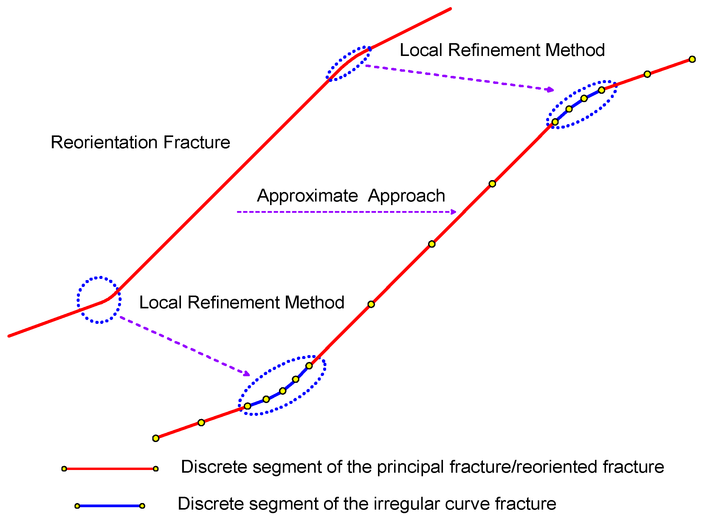
| mi =Total discrete number of all irregular curve fractures |
| Li = The length of the equivalent i-th planar fracture for the irregular curve fracture |
| Lfi,1 = Principal fracture length of the i-th reorientation fracture, m |
| Lfi,2, Lfi,3 = Reoriented fracture length of the i-th reorientation fracture, m |
| △li = length of the i-th fracture segment, i =1, 2…NI, m |
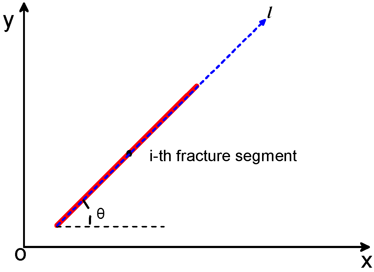
| l = Fracture segment length, m |
| LR = Reference length, m |
| wf = Fracture width, m |
| kx = Permeability in the x-axis, 10-3μm2 |
| ky = Permeability in the y-axis, 10-3μm2 |
| kf = Fracture permeability, 10-3μm2 |
| θi,1 = Principal fracture angle of the i-th reorientation fracture, rad |
| θi,2, θi,3 = Reoriented fracture angle of the i-th reorientation fracture, rad |
| pi = Initial reservoir pressure, MPa |
| ф = Reservoir porosity, fraction |
| u = Fluid viscosity, mPa•s |
| ct = Total compressibility, 1/MPa |
| qsc = Wellbore flow rate, m3/d |
| qfw = Flow rate of a reorientation fracture in the wellbore, m3/d |
| qf = Rate of per unit fracture length from reservoir, m2/d |
| pD = Dimensionless pressure in real time domain |
| = Dimensionless pressure in Laplace domain |
| = Dimensionless reoriented fracture pressure in Laplace domain |
| = Dimensionless flow rate of a reorientation fracture in the wellbore in the Laplace domain |
| = Dimensionless flow rate of per unit fracture length from reservoir in the Laplace domain |
| qfD = Dimensionless flow rate of per unit fracture length from reservoir in the real time domain |
| qD = Dimensionless point source flux |
| FcD = Dimensionless fracture conductivity |
| lD = Dimensionless fracture segment length |
| tD = Dimensionless time |
| xD = Dimensionless distance in the x-axis |
| yD = Dimensionless distance in the y-axis |
| dpwD = Dimensionless pressure derivative |
| xwD = Dimensionless distance in the x-axis of the center of the reservoir |
| ywD = Dimensionless distance in the y-axis of the center of the reservoir |
| RF = Reorientation fracture |
| FR = The location where the fracture reoriented |
| xeD = Dimensionless reservoir length in the x-axis |
| yeD = Dimensionless reservoir width in the y-axis |
| RDk = Dimensionless coefficient |
| s = Dimensionless time variable in Laplace domain |
| NI = Total fracture segment |
| N = Total fracture number |
| △lDi = Dimensionless length of the i-th fracture segment, i =1, 2…NI |
| xDmi = Dimensionless coordinate along the fracture extension |
| yDk = Dimensionless coordinate along the fracture extension |
| cosh = Hyperbolic cosine function |
| sinh = Hyperbolic sine function |
Appendix A. Simplified Algorithm for Discrete Equations of a Reorientation Fracture
References
- Siebrits, E.; Elbel, J.L.; Hoover, R.S.; Diyashev, I.R.; Griffin, L.G.; Demetrius, S.L.; Wright, C.A.; Davidson, B.M.; Steinsberger, N.P.; Hill, D.G. Refracture reorientation enhances gas production in Barnett shale tight gas wells. In Proceedings of the SPE Annual Technical Conference and Exhibition, Dallas, TX, USA, 1–4 October 2000. [Google Scholar]
- Benedict, D.S.; Miskimins, J.L. Analysis of reserve recovery potential from hydraulic fracture reorientation in tight gas Lenticular reservoirs. In Proceedings of the SPE Hydraulic Fracturing Technology Conference, The Woodlands, TX, USA, 19–21 January 2009. [Google Scholar]
- Tang, S.K.; Li, M.Z.; Qi, M.H.; Han, R.; Li, G. Study of fracture reorientation caused by induced stress before re-fracturing. Fault-Block Oil Gas Field 2017, 24, 557–560. [Google Scholar]
- Soliman, M.Y.; Hunt, J.L.; El Rabaa, A.M. Fracturing aspects of horizontal wells. J. Pet. Technol. 1990, 42, 966–973. [Google Scholar] [CrossRef]
- Ozkan, E. Performance of Horizontal Wells. Ph.D. Thesis, Tulsa University, Tulsa, OK, USA, 1988. [Google Scholar]
- Larsen, L.; Hegre, T.M. Pressure-transient behavior of horizontal wells with finite-conductivity vertical fractures. In Proceedings of the International Arctic Technology Conference, Anchorage, AK, USA, 29–31 May 1991. [Google Scholar]
- Larsen, L.; Hegre, T.M. Pressure transient analysis of multi-fractured horizontal wells. In Proceedings of the SPE Annual Technical Conference and Exhibition, New Orleans, LA, USA, 25–28 September 1994. [Google Scholar]
- Chen, C.C.; Raghavan, R. A multiply-fractured horizontal well in a rectangular drainage region. SPE J. 1997, 2, 455–465. [Google Scholar] [CrossRef]
- Zerzar, A.; Bettam, Y. Interpretation of multiple hydraulically-fractured horizontal wells in closed systems. In Proceedings of the SPE International Improved Oil Recovery Conference in Asia Pacific, Kuala Lumpur, Malaysia, 20–21 October 2003. [Google Scholar]
- Wang, J.; Jia, A.; Wei, Y.; Qi, Y. Approximate semi-analytical modeling of transient behavior of horizontal well intercepted by multiple pressure-dependent conductivity fractures in pressure-sensitive reservoir. J. Petrol. Sci. Eng. 2017, 153, 157–177. [Google Scholar] [CrossRef]
- Wright, C.A. Reorientation of propped refreacture treatments in the Lost Hills Field. In Proceedings of the SPE Western Regional Meeting, Long Beach, CA, USA, 23–25 March 1994. [Google Scholar]
- Wright, C.A.; Conant, R.A. Hydraulic fracture reorientation in primary and secondary recovery from low-permeability reservoirs. In Proceedings of the SPE Annual Technical Conference and Exhibition, Dallas, TX, USA, 22–25 October 1995. [Google Scholar]
- Fisher, M.K.; Wright, C.A.; Davison, B.M.; Goodwin, A.K.; Fielder, E.O.; Buckler, W.S.; Steinsberger, N.P. Integrating fracture mapping technologies to optimize stimulations in the Barnett shale. In Proceedings of the SPE Annual Technical Conference and Exhibition, San Antonio, TX, USA, 29 September–2 October 2002. [Google Scholar]
- Fisher, M.K.; Heinze, J.R.; Harris, C.D.; Davidson, B.M.; Wright, C.A.; Dunn, K.P. Optimizing horizontal completion techniques in the Barnett shale using miscoseismic fracture mapping. In Proceedings of the SPE Annual Technical Conference and Exhibition, Houston, TX, USA, 26–29 September 2004. [Google Scholar]
- Restrepo, D.P. Pressure Behavior of a System Containing Multiple Vertical Fractures. Ph.D. Thesis, The University of Oklahoma, Norman, OK, USA, 2008. [Google Scholar]
- Luo, W.J.; Tang, C.F. Pressure-transient analysis of multiwing fractures connected to a vertical wellbore. SPE J. 2015, 20, 360–367. [Google Scholar] [CrossRef]
- Luo, W.J.; Wang, X.; Tang, C.; Feng, C.; Shi, E. Productivity of multiple fractures in a closed rectangular reservoir. J. Petrol. Sci. Eng. 2017, 157, 232–247. [Google Scholar] [CrossRef]
- Tian, Q.; Liu, P.; Jiao, Y.; Bie, A.; Xia, J.; Li, B.; Liu, Y. Pressure transient analysis of non-planar asymmetric fractures connected to vertical wellbores in hydrocarbon reservoirs. Int. J. Hydrogen Energy 2017, 42, 18146–18155. [Google Scholar] [CrossRef]
- Zhou, W.; Banerjee, R.; Poe, B.D.; Spath, J.; Thambynayagam, M. Semianalytical production simulation of complex hydraulic-fracture networks. SPE J. 2012, 19, 6–18. [Google Scholar] [CrossRef]
- Yu, W.; Wu, K.; Sepernoori, K. A semianalytical model for production simulation from nonplanar hydraulic-fracture geometry in tight oil reservoirs. SPE J. 2016, 21, 1028–1040. [Google Scholar] [CrossRef]
- Chen, Z.; Liao, X.; Sepehrnoori, K.; Yu, W. A semi-analytical model for pressure transient analysis of fractured wells in unconventional plays with arbitrarily distributed fracture networks. In Proceedings of the SPE Annual Technical Conference and Exhibition, San Antonio, TX, USA, 9–11 October 2017. [Google Scholar]
- Wu, S.; Xing, G.; Cui, Y.; Wang, B.; Shi, M.; Wang, M. A semi-analytical model for pressure transient analysis of hydraulic reorientation fracture in an anisotropic reservoir. J. Petrol. Sci. Eng. 2019, 153, 157–177. [Google Scholar] [CrossRef]
- Wang, L.; Xue, L. A Laplace-transform boundary element model for pumping tests in irregularly shaped double-porosity aquifers. J. Hydrol. 2018, 567, 712–720. [Google Scholar] [CrossRef]
- Cinco, L.H.; Samaniego, V.F.; Dominguez, A.N. Transient pressure behavior for a well with a finite-conductivity vertical fracture. SPE J. 1978, 18, 253–264. [Google Scholar] [CrossRef]
- Stehfest, H. Algorithm 368: Numerical Inversion of Laplace Transform. Commun. ACM 1970, 13, 47–49. [Google Scholar] [CrossRef]


| Basic Model Parameters | Value |
|---|---|
| Drainage area (dimensionless) | 200 × 200 |
| Fracture conductivity (dimensionless) | 20 |
| Principal fracture angle (deg) | θ1x = θ1y =θ1z = 60° |
| Reoriented fracture angle (deg) | θ2x = θ2y = θ2z = 30° θ3x = θ3y = θ3z = 30° |
| Fracture spacing (dimensionless) | 20 |
| Inner fracture position (dimensionless) | xD = yD = 100 |
© 2019 by the authors. Licensee MDPI, Basel, Switzerland. This article is an open access article distributed under the terms and conditions of the Creative Commons Attribution (CC BY) license (http://creativecommons.org/licenses/by/4.0/).
Share and Cite
Xing, G.; Wu, S.; Wang, J.; Wang, M.; Wang, B.; Cao, J. Pressure Transient Performance for a Horizontal Well Intercepted by Multiple Reorientation Fractures in a Tight Reservoir. Energies 2019, 12, 4232. https://doi.org/10.3390/en12224232
Xing G, Wu S, Wang J, Wang M, Wang B, Cao J. Pressure Transient Performance for a Horizontal Well Intercepted by Multiple Reorientation Fractures in a Tight Reservoir. Energies. 2019; 12(22):4232. https://doi.org/10.3390/en12224232
Chicago/Turabian StyleXing, Guoqiang, Shuhong Wu, Jiahang Wang, Mingxian Wang, Baohua Wang, and Jinjian Cao. 2019. "Pressure Transient Performance for a Horizontal Well Intercepted by Multiple Reorientation Fractures in a Tight Reservoir" Energies 12, no. 22: 4232. https://doi.org/10.3390/en12224232
APA StyleXing, G., Wu, S., Wang, J., Wang, M., Wang, B., & Cao, J. (2019). Pressure Transient Performance for a Horizontal Well Intercepted by Multiple Reorientation Fractures in a Tight Reservoir. Energies, 12(22), 4232. https://doi.org/10.3390/en12224232