Model Predictive Control Tuning by Inverse Matching for a Wave Energy Converter

Abstract

This paper investigates the application of a method to find the cost function or the weight matrices to be used in model predictive control (MPC) such that the MPC has the same performance as a predesigned linear controller in state-feedback form when constraints are not active. This is potentially useful when a successful linear controller already exists and it is necessary to incorporate the constraint-handling capabilities of MPC. This is the case for a wave energy converter (WEC), where the maximum power transfer law is well-understood. In addition to solutions based on numerical optimization, a simple analytical solution is also derived for cases with a short prediction horizon. These methods are applied for the control of an empirically-based WEC model. The results show that the MPC can be successfully tuned to follow an existing linear control law and to comply with both input and state constraints, such as actuator force and actuator stroke.

1. Introduction

Control design for wave energy converters (WECs) is a critical component in the broader WEC design problem. A WEC is generally designed to achieve a desired performance goal, such as maximization of electrical power transferred to the grid while minimizing levelized cost of energy and should survive in extreme ocean environments, under various design constraints. This imposes numerous engineering challenges, comprising environmental characterization, modeling, failure detection, and fatigue analysis. Active control strategies are usually developed to achieve the desired goals, but they are significantly related to the WEC design process in that they alter the overall WEC dynamics in terms of system performance and development costs. Additionally, various types of constraints resulting from WEC design or environmental conditions must be considered when developing control systems.

A number of control design approaches and frameworks have been applied to WECs in the past. In regular waves, maximum energy is captured when the natural frequency of the WEC device is close to the dominant frequency of the incoming wave [1]. At resonance, the velocity of the WEC oscillator is in phase with the excitation force induced by the wave. Complex conjugate (CC) control or impedance matching described in the frequency domain enables this resonance and leads to the theoretically optimal device velocity guaranteeing maximum energy extraction [2]. In realizing this CC control strategy in practice, the main challenge to be overcome is that its general solution is noncausal and thus requires a good prediction for the upcoming wave force. Since the requirement under real irregular sea conditions is that the device should behave as if resonant over the wide range of frequencies, Budal and Falnes [3] proposed the so-called latching control in which the motion of the device is stalled at the extremes of its movement and released when its phase is in good agreement with the wave force. In Korde [4] an efficiency improvement using latching control was demonstrated by conducting an experimental study. In order to expand the efficiency range on either side of the resonant frequency, reactive control [5] was suggested by dynamically adjusting the WEC parameters for maximum energy absorption. Korde [4] showed that the damping coefficient could be adjusted by velocity feedback to maximize permissible energy absorption. In Scruggs et al. [6] the optimal controller was found by solving a nonstandard linear quadratic Guassian optimal control problem. Various other control algorithms have been also applied, including dynamic programming [7], pseudo-spectral methods [8], fuzzy logic control [9], shape-based control [10], moment matching [11], and model predictive control [12].

Among practical control considerations, model predictive control (MPC) possesses a unique feature, in that it takes into account constraints from the beginning of the controller design process [13]. Conversely, the analysis of the stability, robustness, and sensitivity of MPC is more intricate to handle in contrast to linear feedback controllers [14]; these factors often act as the main hurdles for implementation of MPC in real-life applications. Moreover, it is often difficult to find an appropriate cost function for MPC optimization. The vast experience gained from linear controller design can provide many benefits for MPC design and tuning the MPC such that it has the same behavior as a well-designed linear controller when constraints are not active is an attractive approach. Several researchers have attempted to link MPC to an existing linear control law to improve performance due to the constraint-handling capabilities of MPC. In Maciejowski [15] a procedure was presented to construct an observer-based MPC realization of an existing output-feedback controller such that the MPC is equivalent to the given controller when all constraints are inactive. This methodology was extended in Foo and Weyer [16] using a reduced-order observer and state augmentation. Cairano and Bemporad [17] presented approximate solutions for the weight matrices of MPC that behaves as a given linear controller in state-feedback or linear quadratic regulator form in case constraints are inactive by recasting the problem as a convex optimization problem with linear matrix inequality constraints. The global stability of the closed-loop system in the presence of constraints is also guaranteed. Kong et al. [18] further generalized this kind of inverse matching by regarding MPC as a desirable upgrade of an existing control law for performance improvement. Introducing a confidence parameter $\lambda \in [0,1]$, Kong et al. [18] sought how to move smoothly from the existing controller $(\lambda =0)$ to the full MPC strategy $(\lambda =1)$.

In a wave energy perspective, CC control guarantees maximum power absorption with the limitation of noncausality such that a prediction for the wave elevation or the excitation force must be known or sufficiently accurately estimated in advance. In practice, CC control based on prediction is often accomplished via a velocity tracking MPC–this has the added benefit of handling constraints. On the other hand, a feedback controller such as a proportional-integral (PI) controller circumvents this issue and requires only signals/sensors which are readily available, but with the lack of constraint-handling capabilities. Hence, in this paper, we incorporate the linear feedback control designs within MPC frameworks to take into account constraints in an optimal manner by revisiting the inverse matching method in Cairano and Bemporad [17]. A new analytical solution is also proposed that immediately generates optimal weight matrices in MPC for a short prediction horizon case. This approach has a number of advantages compared to the current WEC control strategies. First, predictions of future wave elevation or excitation force are not required for power maximization. The MPC behaves exactly as the predesigned linear controller when constraints are inactive, while satisfying the constraints in an optimal manner when they are active. When constraints are active, MPC acts as a supervisory controller to prevent constraint violations. For a WEC, these constraints can be torque limits of the generator or displacement limits of a linear piston or stage. Second, this approach, differently from all the previous approaches for MPC for WECs (see, e.g., [19]), is in a standard MPC form and thus can be implemented by the software already available (e.g., the Model Predictive Control Toolbox from MathWorks). These are significant practical advantages, as the structure of the controller is simpler and implementing such a solver for real-time control is far from trivial.

To investigate the potential of this approach, we consider a single body one degree-of-freedom (1DOF) WEC. The WEC plant model was estimated from real experimental data including power take-off system dynamics and was described in a linear transfer function form with the control force as the input and the velocity of the buoy as the output [20]. Based on this model, an MPC matching problem is solved to yield proper weight matrices. The MPC designed via the proposed approach behaves exactly as a given PI controller when the control system is unconstrained. When constraints are applied, the MPC retains the general impedance matching dynamics, but also avoids constraint violation.

2. Methods

2.1. Controller Matching Problem

In this section, an MPC algorithm is derived that will behave exactly as the predesigned state-feedback controller when constraints are inactive. In Cairano and Bemporad [17], it was shown that a linear state-feedback controller can be realized via MPC with specially tuned weight matrices—this approach is referred to as MPC inverse matching. For example, a PI controller is a simple example of state feedback control, so we can apply the inverse matching method to obtain an MPC that exactly behaves as the PI controller when constraints are inactive.

In MPC formulation, the following finite-horizon optimal control problem is solved at each sampling time [13,17]

$$\begin{array}{c}\hfill \mathcal{V}(\mathit{x}\left(k\right),\mathit{u}\left(k\right))=\underset{\mathit{U}\left(k\right)}{min}{\mathit{x}}^{\prime }\left(N\right|k)\mathbf{P}\mathit{x}\left(N\right|k)+\\ \hfill \sum _{i=0}^{N-1}{\mathit{x}}^{\prime }\left(i\right|k)\mathbf{Q}\mathit{x}\left(i\right|k)+{\mathit{u}}^{\prime }\left(i\right|k)\mathbf{R}\mathit{u}\left(i\right|k),\end{array}$$

(1)

where the notation ${}^{\prime }$ denotes the transpose of a vector, such that

$$\mathit{x}(i+1|k)=\mathbf{A}\mathit{x}(i\left|k\right)+\mathbf{B}\mathit{u}\left(i\right|k),i=0,\dots ,N-1,$$

(2)

$$x_{min}\le \parallel \mathit{x}\left(i\right|k)\parallel \le x_{max},i=0,\dots ,N,$$

(3)

$$u_{min}\le \parallel \mathit{u}\left(i\right|k)\parallel \le u_{max},i=0,\dots ,N-1,$$

(4)

$$\mathit{x}\left(0\right|k)=\mathit{x}(k),$$

(5)

where Equation (2) is the discrete-time state space equation of the plant model, $\mathit{x}\in {\mathbb{R}}^n$ is the state vector, $\mathit{u}\in {\mathbb{R}}^m$ is the control input vector, $\mathbf{A}$ and $\mathbf{B}$ are the state matrix and the input matrix, respectively, N is the prediction horizon, $\mathit{U}\left(k\right)=[{\mathit{u}}^{\prime }\left(0\right|k)...{\mathit{u}}^{\prime }(N-1|k)]\in {\mathbb{R}}^{Nm}$ is the vector to be optimized, and $\mathcal{V}:{\mathbb{R}}^n\to {\mathbb{R}}_{0+}$ is the value function. The matrices $\mathbf{P}\in {\mathbb{R}}^{n\times n}$, $\mathbf{Q}\in {\mathbb{R}}^{n\times n}$, and $\mathbf{R}\in {\mathbb{R}}^{m\times m}$ are the weight matrices that should be tuned. Assuming that the current state $\mathit{x}\left(k\right)$ is given, the finite horizon optimal control problem Equation (1) can be recast to the following quadratic program (QP) with respect to $\mathit{U}\left(k\right)$

$$\underset{\mathit{U}\left(k\right)}{min}{\mathit{U}}^{\prime }\left(k\right)\mathbf{H}\mathit{U}\left(k\right)+2{\mathit{x}}^{\prime }\left(k\right)\mathbf{F}\mathit{U}\left(k\right)$$

(6)

such that

$$\mathbf{G}\mathit{U}\left(k\right)\le \mathbf{\lambda }+\mathbf{\Lambda }\mathit{x}\left(k\right),$$

(7)

where $\mathbf{G}\in {\mathbb{R}}^{q\times Nm}$, $\mathit{\lambda }\in {\mathbb{R}}^q$, and $\mathbf{\Lambda }\in {\mathbb{R}}^{q\times n}$ are the problem constraints. Also, the following new matrices are defined in Equation (6)

$$\mathbf{H}=\mathcal{R}+{\mathcal{S}}^{\prime }\mathcal{Q}\mathcal{S},\mathbf{F}={\mathcal{T}}^{\prime }\mathcal{Q}\mathcal{S},$$

(8)

where $\mathcal{S}$ is the N-steps state reachability matrix, $\mathcal{T}$ is the N-steps free evolution matrix

$$\mathcal{S}=\left[\begin{array}{cccc}\mathbf{B}& \mathbf{0}& \cdots & \mathbf{0}\\ \mathbf{A}\mathbf{B}& \mathbf{B}& \cdots & \mathbf{0}\\ ⋮& ⋮& \ddots & ⋮\\ {\mathbf{A}}^{N-1}\mathbf{B}& {\mathbf{A}}^{N-2}\mathbf{B}& \cdots & \mathbf{B}\end{array}\right],\mathcal{T}=\left[\begin{array}{c}\mathbf{A}\\ {\mathbf{A}}^2\\ ⋮\\ {\mathbf{A}}^N,\end{array}\right],$$

(9)

and $\mathcal{Q}\in {\mathbb{R}}^{Nn\times Nn}$, $\mathcal{R}\in {\mathbb{R}}^{Nm\times Nm}$ are block-diagonal matrices

$$\mathcal{Q}=\left[\begin{array}{ccccc}\mathbf{Q}& \mathbf{0}& \mathbf{0}& \cdots & \mathbf{0}\\ \mathbf{0}& \mathbf{Q}& \mathbf{0}& \cdots & \mathbf{0}\\ ⋮& ⋮& \ddots & ⋮& ⋮\\ \mathbf{0}& \mathbf{0}& \cdots & \mathbf{Q}& \mathbf{0}\\ \mathbf{0}& \mathbf{0}& \cdots & \mathbf{0}& \mathbf{P}\end{array}\right],\mathcal{R}=\left[\begin{array}{cccc}\mathbf{R}& \mathbf{0}& \cdots & \mathbf{0}\\ \mathbf{0}& \mathbf{R}& \cdots & \mathbf{0}\\ ⋮& ⋮& \ddots & ⋮\\ \mathbf{0}& \cdots & \mathbf{0}& \mathbf{R}\end{array}\right].$$

(10)

When constraints are not active, the QP Eqaution (6) has the unconstrained optimal solution ${\mathit{U}}^{*}\left(k\right)$ which is obtained by solving the Karush–Kuhn–Tucker optimality conditions [21]:

$${\mathit{U}}^{*}\left(k\right)=\left[\begin{array}{c}{\mathit{u}}^{*}\left(0\right|k)\\ ⋮\\ {\mathit{u}}^{*}(N-1|k)\end{array}\right]=-{\mathbf{H}}^{-1}{\mathbf{F}}^{\prime }\mathit{x}\left(k\right),$$

(11)

where the superscript * denotes the optimal values. The MPC command at step k then picks up only the first move such that

$${\mathit{u}}_{\mathrm{MPC}}\left(\mathit{x}\left(k\right)\right)={\mathit{u}}^{*}\left(0\right|k)=-\mathbf{\Gamma }{\mathbf{H}}^{-1}{\mathbf{F}}^{\prime }\mathit{x}\left(k\right),$$

(12)

where $\mathbf{\Gamma }=[{\mathbf{I}}_m\mathbf{0}\cdots \mathbf{0}]$ with the m by m identity matrix ${\mathbf{I}}_m$.

Now, we consider a predesigned linear controller in a state feedback form

$${\mathit{u}}_{\mathrm{LN}}\left(k\right)=\mathbf{K}\mathit{x}\left(k\right),\mathbf{K}\in {\mathbb{R}}^{m\times n}.$$

(13)

Then, the objective is to find weight matrices $\mathbf{P}$, $\mathbf{Q}$, and $\mathbf{R}$ in Equation (1) such that

$$-\mathbf{\Gamma }{\mathbf{H}}^{-1}{\mathbf{F}}^{\prime }=\mathbf{K}$$

(14)

holds, where $\mathbf{K}$ is given.

In brief, once the weight matrices $\mathbf{P}$, $\mathbf{Q}$, and $\mathbf{R}$ are found that satisfy Equation (14) given $\mathbf{K}$, then the MPC with the cost function Equation (1) behaves as the linear controller of the form Equation (13), when the constraints are not active. The weight matrices $\mathbf{P}$, $\mathbf{Q}$, and $\mathbf{R}$ used in $\mathbf{H}$ and $\mathbf{F}$ in Equations (8)–(10) can be calculated using a numerical optimizer such that the error norm of the matrix $\mathbf{\Gamma }{\mathbf{H}}^{-1}{\mathbf{F}}^{\prime }+\mathbf{K}$ is minimized from Equation (14). Cairano and Bemporad [17] reformulated Equation (14) into the following convex problem:

$$\underset{\mathcal{Q},\mathcal{R}}{min}∥(\mathcal{R}+{\mathcal{S}}^{\prime }\mathcal{Q}\mathcal{S})\mathcal{K}+{\mathcal{S}}^{\prime }\mathcal{Q}\mathcal{T}∥,$$

(15)

where

$$\mathcal{K}=\left[\begin{array}{c}\mathbf{K}\\ \mathbf{K}(\mathbf{A}+\mathbf{BK})\\ ⋮\\ \mathbf{K}{(\mathbf{A}+\mathbf{BK})}^{N-1}\end{array}\right].$$

(16)

with a constraint that the Hessian matrix $\mathbf{H}=\mathcal{R}+{\mathcal{S}}^{\prime }\mathcal{Q}\mathcal{S}$ is positive definite. It is noted that in  Equation (16) the elements of $\mathcal{K}$ are arbitrary except for the first one because only the first element is picked up for the MPC command, which was not explicitly stated in Cairano and Bemporad [17]. In this paper, the optimization problem Equation (14) is tackled by solving it using a numerical optimizer YALMIP [22] to obtain optimal weight matrices $\mathbf{P}$, $\mathbf{Q}$, and $\mathbf{R}$. Also, the MPC signal is easily generated using the standard MPC block available in the Model Predictive Control Toolbox of MathWorks [23], and hence, there is no need to implement a custom optimizer to solve the MPC problems in real time. In the MPC Toolbox the KWIK algorithm [24] is used to solve the QP problem and a prediction model is given by a linear function of the current state and the control/excitation input increments [23]. In the next section, as a special case when $N=2$ we derive an analytical solution for $\mathbf{P}$, $\mathbf{Q}$, and $\mathbf{R}$.

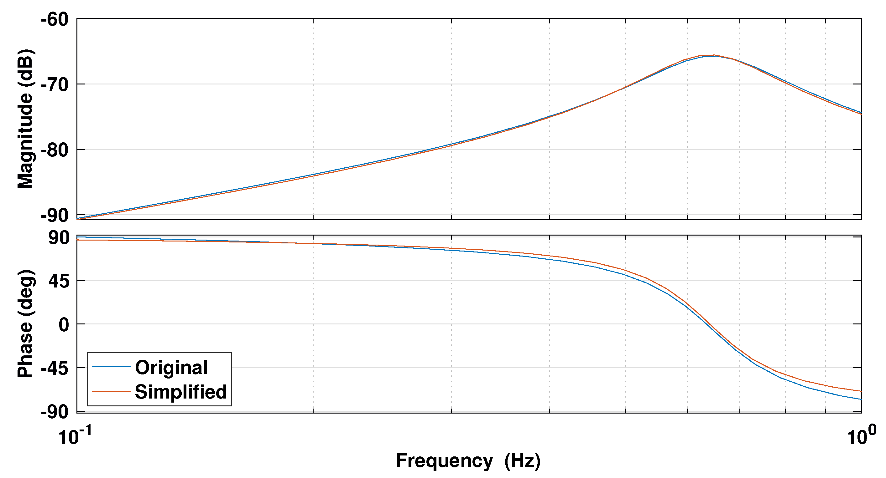
2.2. An Analytical Solution When $N=2$

The optimization problem Eqaution (14) is not trivial to solve because of the existence of the inverse matrix ${\mathbf{H}}^{-1}$ and the non-invertibility of the matrix $\mathbf{\Gamma }$. However, for systems with a one-step prediction ($N=2$) and a single control input ($m=1$), it is possible to derive an analytical solution that immediately generates optimal weight matrices $\mathbf{P}$, $\mathbf{Q}$, and $\mathbf{R}$. A short prediction horizon is sometimes useful because it requires less computational loads and the control performance is independent of the prediction horizon in an unconstrained application. Furthermore, in the area of power electronics and drive, almost all applications use a very short horizon due to the requirement for high speed [25,26]. Since this analytical solution enables immediate calculations for the weight matrices, it is extremely useful in applications in which the weight matrices need to be updated in real time.

When $N=2$, the matrices $\mathcal{S}$, $\mathcal{T}$, $\mathcal{Q}$, and $\mathcal{R}$ in Equations (9) and (10) are simplified as

$$\mathcal{S}=\left[\begin{array}{cc}\mathbf{B}& \mathbf{0}\\ \mathbf{A}\mathbf{B}& \mathbf{B}\end{array}\right],\mathcal{T}=\left[\begin{array}{c}\mathbf{A}\\ {\mathbf{A}}^2\end{array}\right],\mathcal{Q}=\left[\begin{array}{cc}\mathbf{Q}& \mathbf{0}\\ \mathbf{0}& \mathbf{P}\end{array}\right],\mathcal{R}=\left[\begin{array}{cc}\mathbf{R}& \mathbf{0}\\ \mathbf{0}& \mathbf{R}\end{array}\right].$$

(17)

Here, $\mathbf{R}$ is a scalar if a single control input (i.e., $m=1$) is considered. Accordingly, the matrices $\mathbf{H}$ and ${\mathbf{F}}^{\prime }$ in Equation (8) become

$$\begin{array}{c}\hfill \mathbf{H}=\left[\begin{array}{cc}\mathbf{R}+{\mathbf{B}}^{\prime }\mathbf{Q}\mathbf{B}+{\mathbf{B}}^{\prime }{\mathbf{A}}^{\prime }\mathbf{P}\mathbf{A}\mathbf{B}& {\mathbf{B}}^{\prime }{\mathbf{A}}^{\prime }\mathbf{P}\mathbf{B}\\ {\mathbf{B}}^{\prime }\mathbf{P}\mathbf{A}\mathbf{B}& \mathbf{R}+{\mathbf{B}}^{\prime }\mathbf{P}\mathbf{B}\end{array}\right],\\ \hfill {\mathbf{F}}^{\prime }=\left[\begin{array}{c}{\mathbf{B}}^{\prime }\mathbf{Q}\mathbf{A}+{\mathbf{B}}^{\prime }{\mathbf{A}}^{\prime }\mathbf{P}{\mathbf{A}}^2\\ {\mathbf{B}}^{\prime }\mathbf{P}{\mathbf{A}}^2\end{array}\right].\end{array}$$

(18)

Then, the inverse of the $2\times 2$ matrix $\mathbf{H}$ is directly calculated as

$${\mathbf{H}}^{-1}=\frac{1}{\mathbf{D}}\left[\begin{array}{cc}\mathbf{R}+{\mathbf{B}}^{\prime }\mathbf{P}\mathbf{B}& -{\mathbf{B}}^{\prime }{\mathbf{A}}^{\prime }\mathbf{P}\mathbf{B}\\ -{\mathbf{B}}^{\prime }\mathbf{P}\mathbf{A}\mathbf{B}& \mathbf{R}+{\mathbf{B}}^{\prime }\mathbf{Q}\mathbf{B}+{\mathbf{B}}^{\prime }{\mathbf{A}}^{\prime }\mathbf{P}\mathbf{A}\mathbf{B}\end{array}\right],$$

(19)

where the determinant $\mathbf{D}$ is given by

$$\mathbf{D}=(\mathbf{R}+{\mathbf{B}}^{\prime }\mathbf{Q}\mathbf{B}+{\mathbf{B}}^{\prime }{\mathbf{A}}^{\prime }\mathbf{P}\mathbf{A}\mathbf{B})(\mathbf{R}+{\mathbf{B}}^{\prime }\mathbf{P}\mathbf{B})-{\mathbf{B}}^{\prime }{\mathbf{A}}^{\prime }\mathbf{P}\mathbf{B}{\mathbf{B}}^{\prime }\mathbf{P}\mathbf{A}\mathbf{B}.$$

(20)

When $m=1$, we have $\mathbf{\Gamma }=\left[10\right]$ in Equation (12) and should find the matrices $\mathbf{Q}$, $\mathbf{R}$, and $\mathbf{P}$ for given $\mathbf{A}$, $\mathbf{B}$, and $\mathbf{K}$ that satisfy the following equation:

$$\begin{array}{c}\hfill -\mathbf{\Gamma }{\mathbf{H}}^{-1}{\mathbf{F}}^{\prime }=\mathbf{K}=\\ \hfill -\frac{1}{\mathbf{D}}[(\mathbf{R}+{\mathbf{B}}^{\prime }\mathbf{P}\mathbf{B})({\mathbf{B}}^{\prime }\mathbf{Q}\mathbf{A}+{\mathbf{B}}^{\prime }{\mathbf{A}}^{\prime }\mathbf{P}{\mathbf{A}}^2)-{\mathbf{B}}^{\prime }{\mathbf{A}}^{\prime }\mathbf{P}\mathbf{B}{\mathbf{B}}^{\prime }\mathbf{P}{\mathbf{A}}^2].\end{array}$$

(21)

For brevity, consider the following $1\times 2$ gain matrix $\mathbf{K}$ (which can be easily extended to general $1\times n$ cases):

$$\mathbf{K}=\left[K_1{K}_2\right].$$

(22)

Then, since any matrices $\mathbf{Q}$, $\mathbf{R}$, and $\mathbf{P}$ satisfying Equation (21) can be solutions, let us first simplify Equation (21) by choosing $\mathbf{P}$ such that ${\mathbf{B}}^{\prime }\mathbf{P}=\mathbf{0}$. General solutions to ${\mathbf{B}}^{\prime }\mathbf{P}=\mathbf{0}$ are given by

$$\mathbf{P}=(\mathbf{I}-{\left({\mathbf{B}}^{\prime }\right)}^{+}{\mathbf{B}}^{\prime })\mathbf{\Xi },$$

(23)

where ${\left({\mathbf{B}}^{\prime }\right)}^{+}$ is the Moore-Penrose generalized inverse of ${\mathbf{B}}^{\prime }$ and $\mathbf{\Xi }$ is an arbitrary $2\times 2$ matrix. However, for the use of MPC formulation, $\mathbf{P}$ must be positive definite so we select the matrix $\mathbf{\Xi }$ as $\mathbf{\Xi }=\gamma (\mathbf{I}-{\left({\mathbf{B}}^{\prime }\right)}^{+}{\mathbf{B}}^{\prime })$ with a positive constant $\gamma$ such that

$$\mathbf{P}=\gamma {(\mathbf{I}-{\left({\mathbf{B}}^{\prime }\right)}^{+}{\mathbf{B}}^{\prime })}^2=\gamma (\mathbf{I}-{\left({\mathbf{B}}^{\prime }\right)}^{+}{\mathbf{B}}^{\prime }).$$

(24)

Although Equation (24) provides an exact solution to ${\mathbf{B}}^{\prime }\mathbf{P}=\mathbf{0}$, the matrix $(\mathbf{I}-{\left({\mathbf{B}}^{\prime }\right)}^{+}{\mathbf{B}}^{\prime })$ is always rank deficient and $\mathbf{P}$ in Equation (24) is always positive semi-definite, not positive definite. It is for this reason that one additional term is added to Equation (24):

$$\mathbf{P}=\gamma (\mathbf{I}-{\left({\mathbf{B}}^{\prime }\right)}^{+}{\mathbf{B}}^{\prime })+\rho \mathbf{I},$$

(25)

where $\rho$ is a small positive number such that ${\mathbf{B}}^{\prime }\mathbf{P}$ is sufficiently close to the zero matrix.

Once the matrix $\mathbf{P}$ is obtained by Equation (25), ${\mathbf{B}}^{\prime }\mathbf{P}=\mathbf{0}$ (approximately) holds and the determinant $\mathbf{D}$ becomes

$$\mathbf{D}=\mathbf{R}(\mathbf{R}+{\mathbf{B}}^{\prime }\mathbf{Q}\mathbf{B}+{\mathbf{B}}^{\prime }{\mathbf{A}}^{\prime }\mathbf{P}\mathbf{A}\mathbf{B}).$$

(26)

Then, the main Equation (21) to be solved for $\mathbf{Q}$ and $\mathbf{R}$ is simplified as

$$\mathbf{R}\mathbf{K}+{\mathbf{B}}^{\prime }\mathbf{Q}\mathbf{\Phi }+\mathbf{\Psi }=\mathbf{0},$$

(27)

where $\mathbf{\Phi }\triangleq \mathbf{A}+\mathbf{B}\mathbf{K}$ and $\mathbf{\Psi }\triangleq {\mathbf{B}}^{\prime }{\mathbf{A}}^{\prime }\mathbf{P}\mathbf{A}(\mathbf{A}+\mathbf{B}\mathbf{K})$. For the sake of simplicity, let us assume $\mathbf{Q}$ to be diagonal and decompose each matrix as

$$\begin{array}{c}\hfill \mathbf{Q}=\left[\begin{array}{cc}{Q}_1& 0\\ 0& Q_2\end{array}\right],\mathbf{K}=\left[K_1{K}_2\right],\mathbf{A}=\left[\begin{array}{cc}{A}_{11}& A_{12}\\ A_{21}& A_{22}\end{array}\right],\\ \hfill \mathbf{B}=\left[\begin{array}{c}{B}_1\\ B_2\end{array}\right],\mathbf{\Phi }=\left[\begin{array}{cc}{\mathrm{\Phi }}_{11}& {\mathrm{\Phi }}_{12}\\ {\mathrm{\Phi }}_{21}& {\mathrm{\Phi }}_{22}\end{array}\right],\mathbf{\Psi }=\left[{\mathrm{\Psi }}_1{\mathrm{\Psi }}_2\right],\end{array}$$

(28)

and R is a scalar because only one control input is considered. Substituting Equation (28) into Equation (27) yields the following equation:

$$\left[\begin{array}{ccc}{K}_1& B_1{\mathrm{\Phi }}_{11}& B_2{\mathrm{\Phi }}_{21}\\ K_2& B_1{\mathrm{\Phi }}_{12}& B_2{\mathrm{\Phi }}_{22}\end{array}\right]\left[\begin{array}{c}R\\ Q_1\\ Q_2\end{array}\right]=-\left[\begin{array}{c}{\mathrm{\Psi }}_1\\ {\mathrm{\Psi }}_2\end{array}\right].$$

(29)

There are three unknowns (R, $Q_1$, $Q_2$) and two equations, and hence, there exist infinite number of solutions. For brevity, let us assume $Q_2=\eta Q_1$ with some constant $\eta$ and Equation (29) becomes

$$\left[\begin{array}{cc}{K}_1& B_1{\mathrm{\Phi }}_{11}+\eta B_2{\mathrm{\Phi }}_{21}\\ K_2& B_1{\mathrm{\Phi }}_{12}+\eta B_2{\mathrm{\Phi }}_{22}\end{array}\right]\left[\begin{array}{c}R\\ Q_1\end{array}\right]=-\left[\begin{array}{c}{\mathrm{\Psi }}_1\\ {\mathrm{\Psi }}_2\end{array}\right].$$

(30)

Then, the solution to Equation (30) is easily found as

$$\left[\begin{array}{c}R\\ Q_1\end{array}\right]=-{\left[\begin{array}{cc}{K}_1& B_1{\mathrm{\Phi }}_{11}+\eta B_2{\mathrm{\Phi }}_{21}\\ K_2& B_1{\mathrm{\Phi }}_{12}+\eta B_2{\mathrm{\Phi }}_{22}\end{array}\right]}^{-1}\left[\begin{array}{c}{\mathrm{\Psi }}_1\\ {\mathrm{\Psi }}_2\end{array}\right].$$

(31)

There are two requirements that must be satisfied such that the obtained matrices $\mathbf{P}$, $\mathbf{Q}$, and $\mathbf{R}$ are valid solutions to Equation (14): the invertibility of the coefficient matrix in Equation (30) and the positive definiteness of the Hessian matrix $\mathbf{H}=\mathcal{R}+{\mathcal{S}}^{\prime }\mathcal{Q}\mathcal{S}$. First, the invertibility of the coefficient matrix in Equation (30) is guaranteed when its determinant is nonzero such that

$$\eta \ne \frac{B_1(K_1{\mathrm{\Phi }}_{12}-K_2{\mathrm{\Phi }}_{11})}{B_2(K_2{\mathrm{\Phi }}_{21}-K_1{\mathrm{\Phi }}_{22})}$$

(32)

or

$$\eta \ne \frac{B_1(A_{12}{K}_1-A_{11}{K}_2)}{B_2(A_{21}{K}_2-A_{22}{K}_1)}$$

(33)

with the definition $\mathbf{\Phi }\triangleq \mathbf{A}+\mathbf{B}\mathbf{K}$. Here, it is assumed $B_2(A_{21}{K}_2-A_{22}{K}_1)\ne 0$. If $B_2(A_{21}{K}_2-A_{22}{K}_1)=0$, we assume $Q_1=\eta Q_2$ instead and follow the same procedure with the assumption $B_1(A_{12}{K}_1-A_{11}{K}_2)\ne 0$. If $B_2(A_{21}{K}_2-A_{22}{K}_1)=0$ and $B_1(A_{12}{K}_1-A_{11}{K}_2)=0$ are satisfied simultaneously, there is generally no solution to Equation (30). Next, for the positive definiteness of the Hessian matrix $\mathbf{H}=\mathcal{R}+{\mathcal{S}}^{\prime }\mathcal{Q}\mathcal{S}$ we simplify the matrix $\mathbf{H}$ in Equation (18) with the condition ${\mathbf{B}}^{\prime }\mathbf{P}=\mathbf{0}$ by

$$\begin{array}{c}\hfill \mathbf{H}=\left[\begin{array}{cc}R+{\mathbf{B}}^{\prime }\mathbf{Q}\mathbf{B}+{\mathbf{B}}^{\prime }{\mathbf{A}}^{\prime }\mathbf{P}\mathbf{A}\mathbf{B}& 0\\ 0& R\end{array}\right].\end{array}$$

(34)

Hence, we obtain two conditions for the requirement $\mathbf{H}>\mathbf{0}$ as

$$R>0,R+{\mathbf{B}}^{\prime }\mathbf{Q}\mathbf{B}=R+B_1^2{Q}_1+B_2^2{Q}_2>-{\mathbf{B}}^{\prime }{\mathbf{A}}^{\prime }\mathbf{P}\mathbf{A}\mathbf{B}.$$

(35)

It is noted that $-{\mathbf{B}}^{\prime }{\mathbf{A}}^{\prime }\mathbf{P}\mathbf{A}\mathbf{B}$ is a negative constant since $\mathbf{P}$ is positive definite. Then, two free parameters $\eta$ and $\gamma$ can be determined that satisfy the two requirements Equations (33) and (35). In general, by picking up a large $\gamma$ and making $-{\mathbf{B}}^{\prime }{\mathbf{A}}^{\prime }\mathbf{P}\mathbf{A}\mathbf{B}$ negative with a large magnitude, we can easily find $\eta$. Hence, we have obtained the explicit solutions for $\mathbf{P}$, $\mathbf{Q}$, and $\mathbf{R}$ that are given in Equations (25) and (31), respectively.

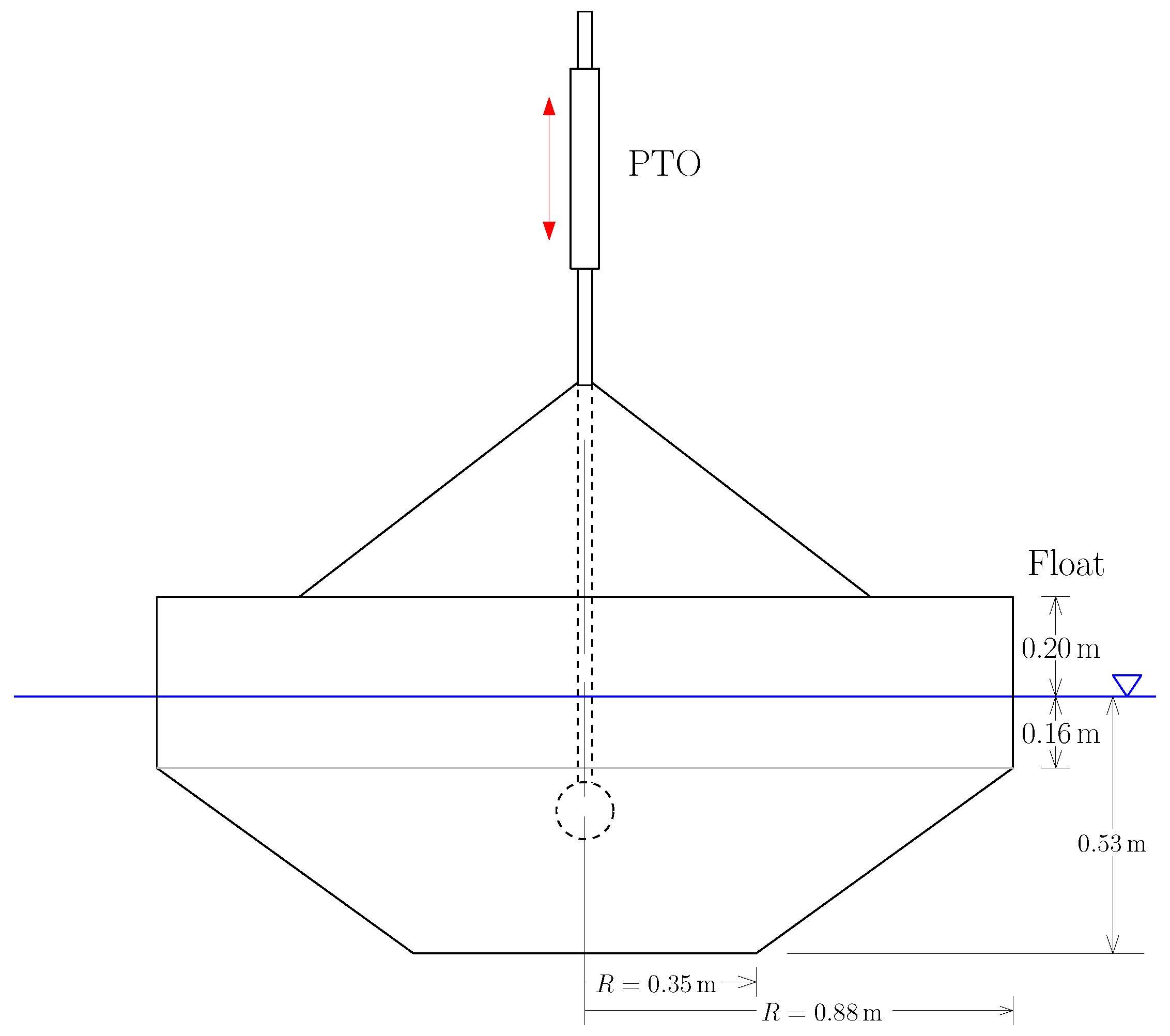
3. Results: Application to a WEC

The MPC matching problem handled in the previous sections can be applied to a WEC control problem, assuming that a successful feedback controller is already in hand. First, we solve the MPC matching problem and verify the solutions via numerical simulations with the estimated WEC model. Next, constraints on the actuator force and the output are considered.

A model-scale heaving point absorber designed at Sandia National Laboratories (for details see [27]) was considered for the case study discussed herein. This device was designed to be 1/17th a full-scale equivalent WEC.  Figure 1 and

Table 1. Model-scale wave energy converter (WEC) physical parameters.

Parameter	Value
Rigid-body mass (float & slider), M (kg)	858
Displaced volume, ∀ (m${}^3$)	0.858
Float radius, r (m)	0.88
Float draft, T (m)	0.53
Water density, $\rho$ (kg/m${}^3$)	1000
Water depth, h (m)	6.1
Linear hydrostatic stiffness, S (kN/m)	23.9
Infinite-frequency added mass, $m_{\infty }$ (kg)	782
Max vertical travel, $\left|z_{\max }\right|$ (m)	0.6

show a diagram of the WEC device and its relevant physical parameters.

The WEC device is modeled in a transfer function form as follows:

$$G_o\left(s\right)=\frac{0.0002371s^3+0.01783s^2-0.002049s}{s^4+24.7s^3+54.53s^2+389.2s+62.92},$$

(36)

which relates the applied actuator control force (input) and the resulting velocity of the WEC device in vertical motion (output). Note that this model does not include the excitation dynamics, which are not necessary for the control approach consider here. (The excitation force model is used only in the simulation of the controller.) To simplify the problem, let us replace the fourth-order model (36) with the following second-order approximation:

$$G_s\left(s\right)=\frac{0.0007293s}{s^2+1.38s+16.2}.$$

(37)

The simplified model (37) was obtained by the MATLAB command tfest over the frequency range of interest $f\in [0.11.0]$ (Hz) assuming that the energy in ocean waves lies within a relatively narrow frequency band (periods of $1\le T\le 10$ s). Note that, as previously stated, the WEC considered here is a model scale device, which is tested in a wave basin. As such, the frequency range of interest is higher than that of an open ocean device. From the second-order model (37), the natural frequency and the damping ratio are found by ${\omega }_n=\sqrt{16.2}$ = 4.025 (rad/s) = 0.641 (Hz) and $\zeta =1.38/\left(2{\omega }_n\right)=0.171$, respectively. Hence, the resonant frequency is located at ${\omega }_n\sqrt{1-2{\zeta }^2}$ = 3.905 (rad/s) = 0.622 (Hz), which is an approximate value because of the existence of the zero in the transfer function. At the resonant frequency, the output is in phase with the input, and for small input frequencies, 90 degrees phase lead occurs while 90 degrees phase lag occurs for large input frequencies.  Figure 2 shows the Bode diagram of the original model (36) and the simplified model (37), which shows a good agreement between the two models. Hence, we proceed to MPC design based on the simplified model (37).

First, we transform Equation (37) to a state-space equation:

$$\dot{\mathit{x}}\left(t\right)={\mathbf{A}}_{\mathbf{c}}\mathit{x}\left(t\right)+{\mathbf{B}}_{\mathbf{c}}\mathbf{u}\left(t\right),\mathbf{y}\left(t\right)={\mathbf{C}}_{\mathbf{c}}\mathit{x}\left(t\right),$$

(38)

where $\mathit{x}\left(t\right)={\left[z\left(t\right)v\left(t\right)\right]}^{\prime }$ is the state vector, $z\left(t\right)$ and $v\left(t\right)$ are the vertical position and velocity of the WEC device, respectively. The coefficient matrices of this system are

$${\mathbf{A}}_{\mathbf{c}}=\left[\begin{array}{cc}0& 1\\ -16.2& -1.38\end{array}\right],{\mathbf{B}}_{\mathbf{c}}=\left[\begin{array}{c}0\\ 0.0007293\end{array}\right],{\mathbf{C}}_{\mathbf{c}}=\left[01\right].$$

(39)

The state Equation (38) is described in continuous time but it must be converted to a discrete-time equation for MPC formulation:

$$\mathit{x}(k+1)=\mathbf{A}\mathit{x}\left(k\right)+\mathbf{B}\mathit{u}\left(k\right),\mathit{y}\left(k\right)=\mathbf{C}\mathit{x}\left(k\right),$$

(40)

where $·\left(k\right)$ is a quantity at the time step k and $\mathit{x}\left(k\right)={\left[z\left(k\right)v\left(k\right)\right]}^{\prime }$, and

$$\mathbf{A}=\left[\begin{array}{cc}0.9968& 0.01971\\ -0.3193& 0.9696\end{array}\right],\mathbf{B}=\left[\begin{array}{c}1.444\times {10}^{-7}\\ 1.437\times {10}^{-5}\end{array}\right],\mathbf{C}=\left[01\right].$$

(41)

where the sampling interval $T_s=0.02$ s is assumed.

Let us assume that the incoming wave is of JONSWAP type spectrum with a peak period of 3.5 s, a significant wave height of 0.254 m, and a peak enhancement factor of 1. Then, with the plant model Equation (37) or Equation (40), the optimal PI controller that maximizes the energy extraction from the wave is given by

$${\mathit{u}}_{PI}\left(k\right)=\mathbf{K}\mathit{x}\left(k\right)=\left[K_1{K}_2\right]\left[\begin{array}{c}z\left(k\right)\\ v\left(k\right),\end{array}\right]$$

(42)

where the gain matrix is calculated as

$$\mathbf{K}=\left[K_1{K}_2\right]=\left[2389-3213\right],$$

(43)

which extracts maximum energy from the incoming wave. The tuning of the PI controller is suboptimal but very close to optimum [27].

3.1. Numerical Simulations

To examine the performance of this controller, we design an MPC that behaves exactly as the PI controller Equation (42) for three different scenarios (see

Table 2. Constraints and prediction horizons (N) of three scenarios.

Scenario	Constraint	ECR Values	N
1	No constraint	N/A	2
2	Nearly hard constraint on position $\in [-0.10.1]$	OV.minECR = OV.maxECR = $2\times {10}^{-4}$	50
3	Hard constraint on control input $\in [-15001500]$ Soft constraint on position $\in [-0.10.1]$	MV.minECR = MV.maxECR = 0 OV.minECR = OV.maxECR = 0.01	50

for a summary of the scenarios) and evaluate that controller in numerical simulations.

• The system has no constraints.
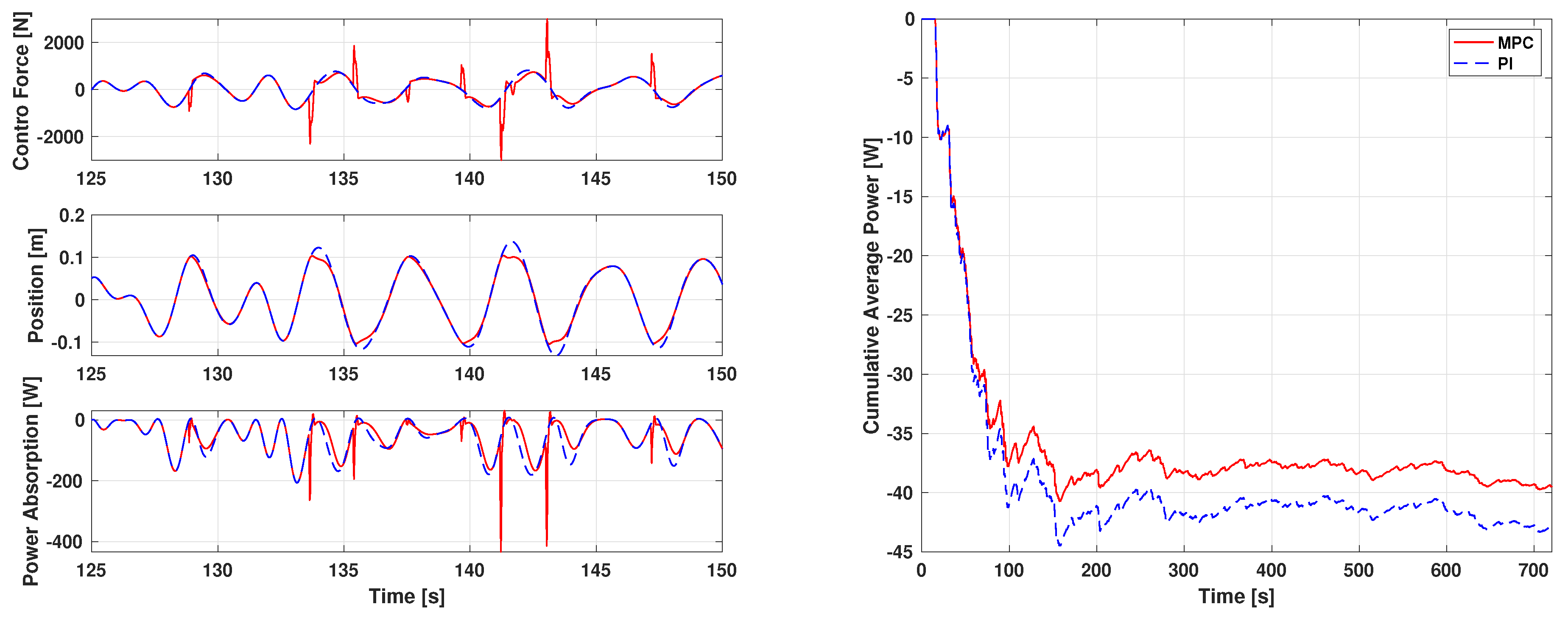
• The system has a nearly hard constraint on its position.
• The system has a hard constraint on its control input and a soft constraint on its position.

More specifically, in Scenario 2 both OV.minECR and OV.maxECR values (OV denotes the output variable) for the position used in the MPC Toolbox are set as $2\times {10}^{-4}$, where an equal concern for the relaxation (ECR) value is zero for a completely hard constraint and a larger ECR value means a softer constraint. When constraints are imposed, the value function Equation (1) is rewritten as

$$\begin{array}{c}\hfill \mathcal{V}(\mathit{x}\left(k\right),\mathit{u}\left(k\right))=\underset{\mathit{U}\left(k\right)}{min}{\mathit{x}}^{\prime }\left(N\right|k)\mathbf{P}\mathit{x}\left(N\right|k)+\\ \hfill \sum _{i=0}^{N-1}{\mathit{x}}^{\prime }\left(i\right|k)\mathbf{Q}\mathit{x}\left(i\right|k)+{\mathit{u}}^{\prime }\left(i\right|k)\mathbf{R}\mathit{u}\left(i\right|k)+\mu {ϵ}_k^2,\end{array}$$

(44)

where $\mu$ is the weight for constraints and ${ϵ}_k(\ge 0)$ is another free optimization variable to be determined. By default,

$$\mu ={10}^{5}max\left\{P_{i,j},Q_{i,j},R_{i,j}\right\},$$

(45)

where $W_{i,j}$ ($\mathbf{W}=\mathbf{P},\mathbf{Q},\mathbf{R}$) is the ($i,j$) component of the matrix $\mathbf{W}$ [23]. The constraints Equations (3) and (4) change to

$$x_{min}+{ϵ}_k{V}_{min}^x\le \parallel \mathit{x}\left(i\right|k)\parallel \le x_{max}+{ϵ}_k{V}_{max}^x,i=0,\dots ,N,$$

(46)

$$u_{min}+{ϵ}_k{V}_{min}^u\le \parallel \mathit{u}\left(i\right|k)\parallel \le u_{max}+{ϵ}_k{V}_{max}^u,i=0,\dots ,N-1,$$

(47)

where $V_{min}^x$, $V_{max}^x$, $V_{min}^u$, and $V_{max}^u$ are the ECR parameters, each of which has the command OV.minECR, OV.maxECR, MV.minECR, and MV.maxECR, respectively in the MPC Toolbox. It is easy to see that when an ECR value is zero, the constraint is a hard one that cannot be violated. The larger ECR value is, the softer the constraint is.

In Scenario 3 both MV.minECR and MV.maxECR values (MV denotes the manipulated variable) are set as 0 for the control input and OV.minECR = OV.maxECR = 0.01 are selected for the position. For all scenarios, the control horizon is equal to the prediction horizon N. It should be mentioned that the parameters are scaled to improve numerical accuracy.

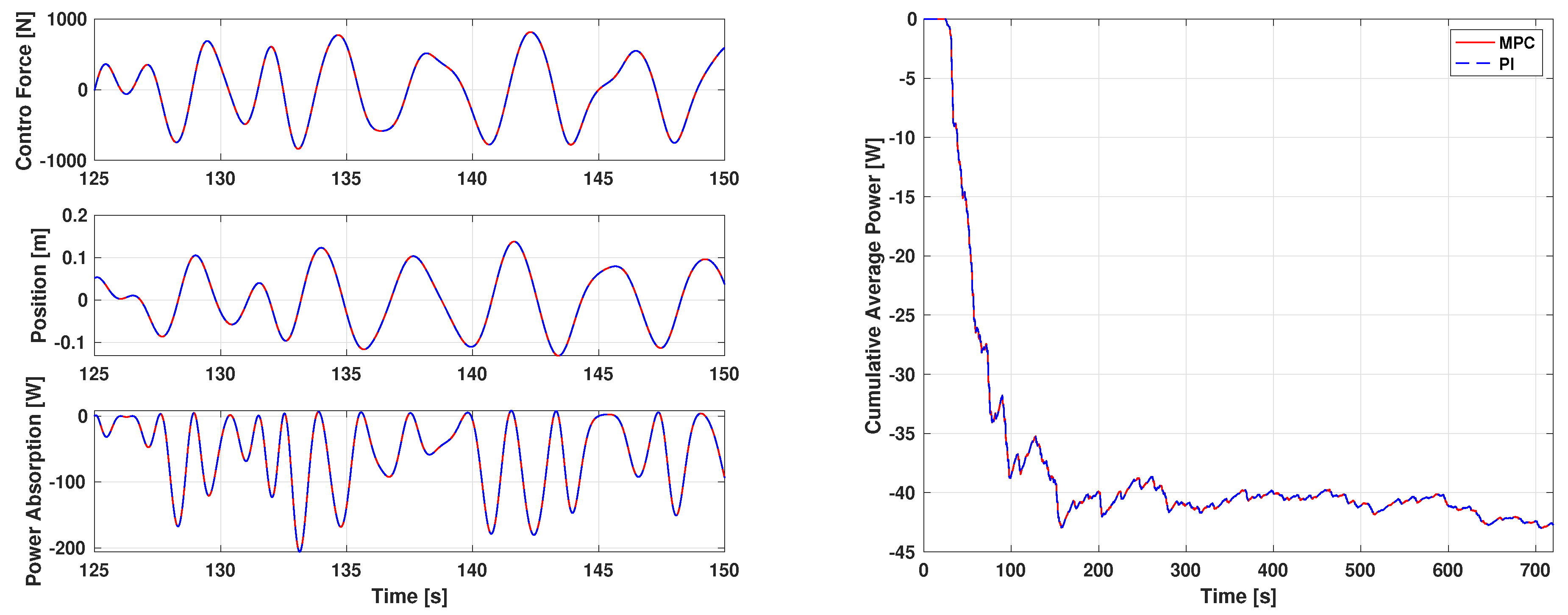
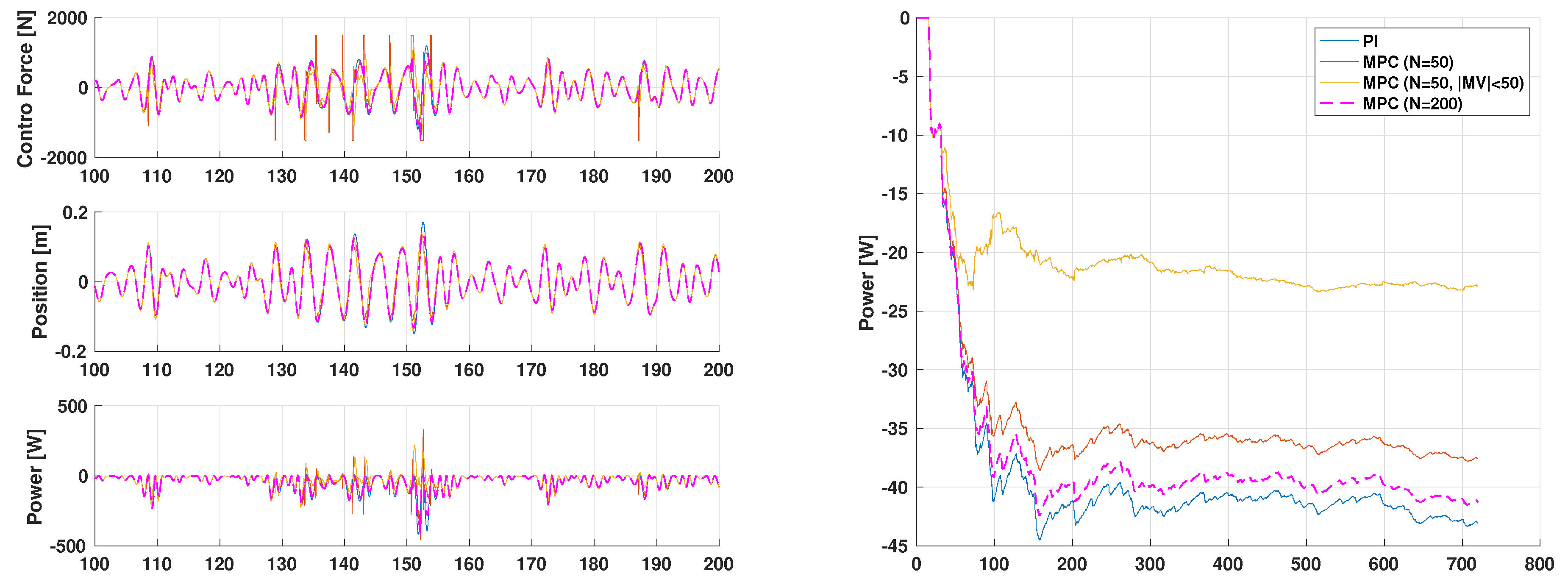
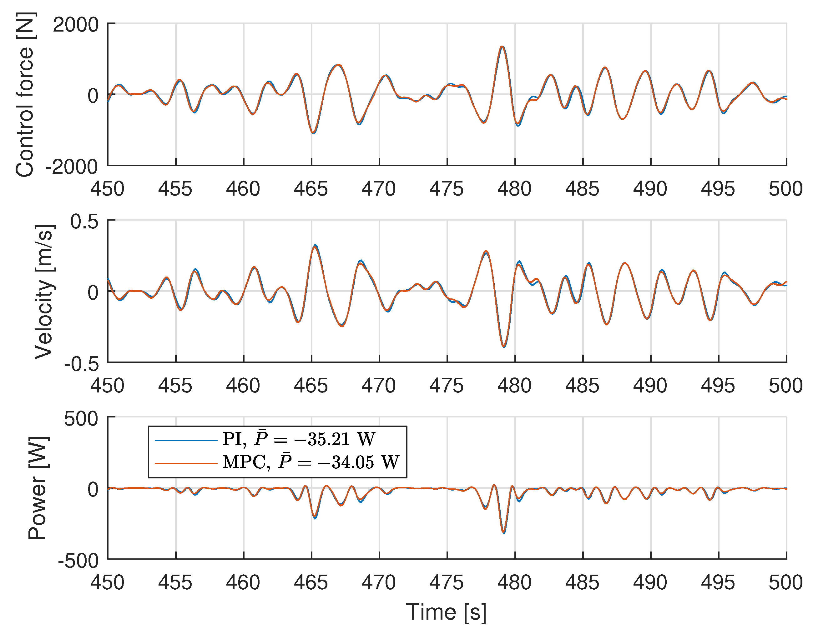
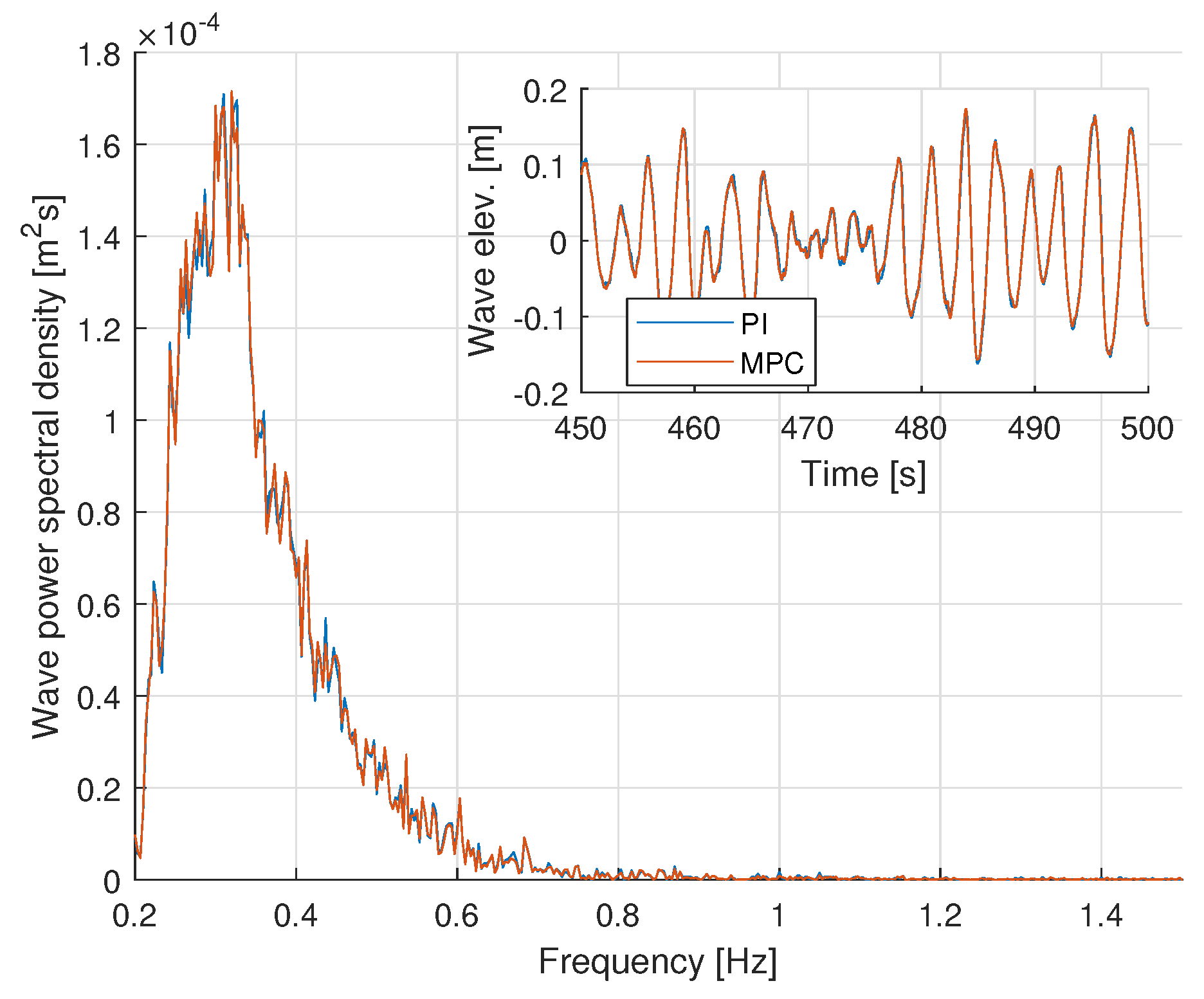
3.1.1. Scenario 1: System with No Constraint

First, we consider an unconstrained case and apply the analytical solution with $N=2$. Since there is no constraint in the system, the performance will be independent of the selection of N [23]. The matrix $\mathbf{P}$ is calculated by (25) with $\gamma ={10}^6$ and $\rho ={10}^{-6}$:

$$\mathbf{P}=\left[\begin{array}{cc}999,899& -10,050\\ -10,050& 101\end{array}\right].$$

(48)

Next, the matrices $\mathbf{Q}$ and $\mathbf{R}$ are calculated by (31) with $\eta =1$:

$$\mathbf{Q}=\left[\begin{array}{cc}-49,339& 0\\ 0& -49,339\end{array}\right],\mathbf{R}=22,149.$$

(49)

Then, the resulting gain matrix $-\mathbf{\Gamma }{\mathbf{H}}^{-1}{\mathbf{F}}^{\prime }$ is calculated as

$$-\mathbf{\Gamma }{\mathbf{H}}^{-1}{\mathbf{F}}^{\prime }=[2388.9999-3012.9999],$$

(50)

which is very close to the original gain $\mathbf{K}$. Also, it is easily checked that the product of $\mathbf{P}$ and the matrix $\mathbf{B}$ in Equation (41) has the norm of the order of ${10}^{-7}$, which validates the accuracy of the analytical solution.

 Figure 3 compares the time histories of the control forces, positions, power absorptions, and cumulative average power obtained by the PI controller and the MPC. The power absorption was defined as the product of the control force and the velocity of the device at each time. Note that the convention of this paper is to show absorbed power as negative power. Because the obtained gain is very similar to the original one, there are only minor differences between the two controllers. For the control forces, positions, and power absorptions (shown in the left-hand pane of  Figure 3), only the time window [125,150] (s) is displayed for a clear view. The average power capture is −42.74 W for both controllers. The right-hand pane in  Figure 3 shows the cumulative average power. Again, we can see that the two controllers perform quite similarly.

3.1.2. Scenario 2: System with Nearly Hard Constraint on the Position

In this scenario, a nearly hard constraint (OV.minECR = OV.maxECR = $2\times {10}^{-4}$) is imposed on the position of the WEC device and the prediction horizon $N=50$ is assumed to anticipate constraint violation early enough to allow corrective action. A ‘nearly’ hard constraint means that the constraint is quite well satisfied on the whole but a small constraint violation is allowed. In practice, a completely hard constraint should not be imposed on the output because the plant is always subject to disturbance and QP infeasibility is inevitable. We apply the numerical solver ‘YALMIP’ to yield the following weight matrices:

$$\begin{array}{c}\hfill \mathbf{P}=\left[\begin{array}{cc}0.44& -28\\ -28& 1788\end{array}\right],\\ \hfill \mathbf{Q}=\left[\begin{array}{cc}-10,160,795& 0\\ 0& 3,338,885\end{array}\right],\mathbf{R}=1.67.\end{array}$$

(51)

Then, the resulting gain matrix $-\mathbf{\Gamma }{\mathbf{H}}^{-1}{\mathbf{F}}^{\prime }$ is calculated as

$$-\mathbf{\Gamma }{\mathbf{H}}^{-1}{\mathbf{F}}^{\prime }=[2389.05-3212.99],$$

(52)

which is very close to the original gain $\mathbf{K}$. More explicitly, the norm of the matrix difference $\mathbf{\Gamma }{\mathbf{H}}^{-1}{\mathbf{F}}^{\prime }+\mathbf{K}$ is calculated as 0.052.

Now, we impose a nearly hard output constraint such that the position should not exceed 0.1 m in both directions.  Figure 4 compares the time histories of the control forces, positions, power absorptions, and cumulative average power obtained by the unconstrained PI controller and the MPC with the output (position) constraint. When the constraint becomes active, the control force has a sudden rise to satisfy the constraint and is released immediately after the constraint turns to inactive. As with almost any system, such behavior is undesirable in a WEC, as it may excite high frequency structural responses and create unnecessary loading. This sudden rise can be relaxed by allowing soft constraints or introducing a longer prediction horizon as will be shown in the next subsection. It is shown that the constraint on the position is satisfied quite accurately. Also, as expected, a constrained system extracts less energy due to the limited motion. However, the reduction in power to satisfy the constraint is quite small: the unconstrained PI controller captures the power of −42.74 W on average for one period of the incoming wave while the constrained MPC captures the power of −39.51 W.

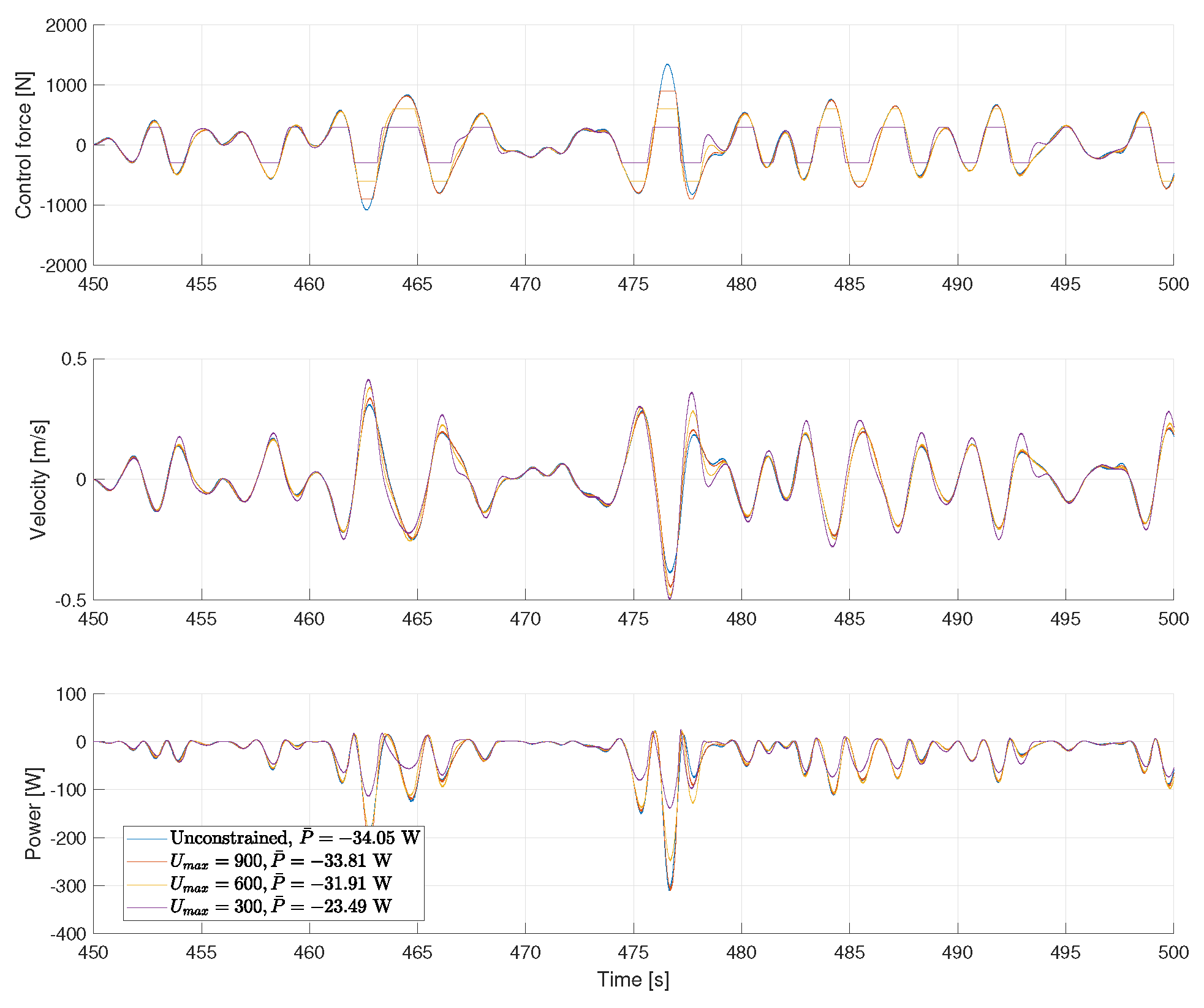
3.1.3. Scenario 3: System with Hard Constraint on the Control Force and Soft Constraint on the Position

As the final scenario, we apply a hard constraint (MV.minECR = MV.maxECR = 0) on the control force and a soft constraint (OV.minECR = OV.maxECR = 0.01) on the position. In general, control force and position constraints cannot always be simultaneously satisfied, and so the position constraint is usually softened for QP feasibility [23]. Bacelli and Ringwood [28] extended the discussion of the force and position constraints for WECs and proposed sufficient conditions for the satisfaction of both constraints for a given hydrodynamic model and set of sea conditions.

Figure 5 compares the time histories of the control forces, positions, power absorptions, and cumulative average power obtained by the unconstrained PI controller and the MPC with the hard and soft constraints. Three different MPCs with these constraints are shown; these controllers are summarized in

Table 3. Comparison of results for Scenario 3.

Name	Prediction Steps	Slew Rate Limit	Power Absorbed [W]
PI	N/A	N/A	−42.7
MPC ($N=50$)	50	(None)	−37.6
MPC ($N=50$, $\left|\mathrm{MV}\right|<50$)	50	$\left|\mathrm{MV}\right|<50$	−22.8
MPC ($N=200$)	200	(None)	−41.2

. In addition to the basic MPC (“MPC ($N=50$)”), there are two additional MPCs that attempt to reduce the large spikes observed in the control force. The first of these (“MPC ($N=50$, $\left|\mathrm{MV}\right|<50$)”) limits the slew rate, that is the rate change of the control force. We can see from Figure 5 that this controller partially reduces the peaks in controller force, but has a rather large effect on power absorption. A third MPC (“MPC ($N=200$)”) uses 200 prediction steps instead of 50. This controller avoids the large spikes in control force with only a small effect on power. In fact, the “MPC ($N=200$)” controller has better power absorption than “MPC ($N=50$).”

3.2. Experimental Tests

The obtained MPC algorithms are now applied to real experiments. The experiments were conducted in the US Navy’s Maneuvering and Sea Keeping (MASK) basin, operated by the Naval Surface Warfare Center, Carderock Division (NSWCCD) in Bethesda, Maryland. The data collected are publicly available at https://mhkdr.openei.org. For the details about the test device, hardware setup, and the wave basin, refer to Coe et al. [27]. As before, two controllers are considered: PI controller and MPC that approximates the PI controller. The WEC system is disturbed by the same JONSWAP type wave used for the numerical simulations. Two identical wave trains were run: one in which the PI controller was used and one in which the MPC was used. A sampling interval $T_s=0.001$ s and a prediction horizon $N=2$ are used for the controllers and the commanded gains for the PI controller are selected as

$$\mathbf{K}=\left[K_I{K}_P\right]=\left[2400-3200\right].$$

(53)

In order to check the control performance a metric $K_{FIT}$ was calculated by estimating the $K_I$ and $K_P$ gains back from the data and comparing them with the actual gains of the PI controller used for the test. This metric is defined by

$$K_{FIT}\triangleq \left(1-\sqrt{{\left(\frac{{\tilde{K}}_I-K_I}{K_I}\right)}^2+{\left(\frac{{\tilde{K}}_P-K_P}{K_P}\right)}^2}\right)\times 100,$$

(54)

where ${\tilde{K}}_I$ and ${\tilde{K}}_P$ are the integral and proportional gains, respectively, estimated from the data and $K_I$ and $K_P$ are the commanded gains shown in Equation (53). The gains were estimated by dividing the measured control force by the measured position and velocity and then picking up the constant optimal values that minimize the fitting error. The estimated gains are

$$\tilde{\mathbf{K}}=[{\tilde{K}}_I{\tilde{K}}_P]=\left[2388-3213\right].$$

(55)

The error norm between Equations (55) and (53) is calculated as $∥\tilde{K}-K∥/∥K∥=0.0044$. Also, the metric (54) is calculated as 99.36%, which shows good agreement between the two controllers.

The top-most plot in Figure 6 displays the time history of the control signals generated by the PI controller and the MPC, which verifies that the MPC behaves as the PI controller on the whole. In order to ensure that the two controllers (PI and MPC) were influenced by the same external wave, the wave elevation data collected from the PI controller and MPC experiments are plotted in the frequency domain and compared in Figure 7. In the inset, the wave elevation data in time domain are plotted for reference. The wave elevation was measured by a sensor that was located far enough from the buoy so that any radiation effect from the buoy could be ignored. Figure 7 shows that the two controllers were indeed under the quite similar wave forces. In the middle plot in Figure 6, the time history of the velocities of the WEC device obtained by the PI controller and the MPC is depicted. Since the control signal of the MPC closely emulates the PI control signal and the two controllers were influenced by the same wave force, the two velocities are also similar. The lower plot in Figure 6 displays the time history of the power captured by using the PI controller and the MPC. The average power ($\overline{P}$) captured by the PI controller and the MPC is −35.21 W and −34.05 W, respectively, which also shows the performance difference of the two controllers is small (3%).

Now, we consider constrained MPCs such that the control signal is saturated with given upper/lower limits (assuming hard constraints). It will also be shown that the power captured by the constrained MPC is reduced only by a small amount when compared with the unconstrained MPC even though a very short prediction horizon $N=2$ is used. Let us say that $U_{max}$ is the maximum control magnitude that can be reached by the actuator. Since the maximum control magnitude is found to be about 1200 N from the top-most plot in Figure 6, let us constrain the system by forcing $U_{max}$ to be 900, 600, and 300 N.

As with the previous example, experiments were run with the same wave input; in each of the four cases, the maximum control input was set to $U_{max}=\left[1200900600300\right]$ (N). The top-most plot in Figure 8 shows the control forces obtained by these unconstrained and constrained MPCs. It is clear that the control forces successfully stay within the desired range. In the middle plot in Figure 8, the resulting velocities are plotted for the unconstrained and constrained MPCs. With the constrained MPCs, the magnitude of the resulting velocity is greater than the unconstrained case because the saturated control force cannot fully regulate the velocity. The lower plot in Figure 8 displays the time history of the power captured by using the unconstrained and constrained MPCs. As expected, when the constraint is active, less power is captured.

However,

Table 4. Power captured (W and % change from unconstrained) by using unconstrained and constrained MPCs.

Controller	Power Capture [W]	% Reduction
Unconstrained	−34.1	0
$U_{max}=900$ N (75%)	−33.8	0.7
$U_{max}=600$ N (50%)	−31.9	6.3
$U_{max}=300$ N (25%)	−23.5	31.0

indicates that the power captured by the constrained MPCs is worse only by a small percentage when compared with the unconstrained MPC. In the Table 4, the average power capture obtained using the unconstrained and constrained MPCs is listed and the power loss in percentage is also presented in the parenthesis compared with the unconstrained case. For example, when the control force is constrained with $U_{max}=600$ which corresponds to 50% of the maximum control magnitude obtained when the unconstrained MPC is applied, the power capture is −31.91 W, which is worse only by 6.28% compared with the unconstrained case (−34.05 W) despite the fact that a very short horizon $N=2$ is employed.

4. Conclusions

This paper studies the application of MPC tuning methods via inverse matching to a WEC, such that the MPC behaves exactly like a predesigned linear controller when constraints are inactive. With the PI controller and device model obtained from real experimental data, the MPC behaved exactly as the PI controller when constraints are not active. When constraints are active, the MPC can be designed to follow them to the desired degree. A predesigned causal predictionless controller was easily realized via MPC technique with specially tuned weight matrices. This controller requires only signals/sensors that are readily available such as position/velocity. By incorporating it within MPC frameworks, the ability to incorporate constraints is successfully maintained. In addition to numerical simulations, experimental results show both accuracy and feasibility of this method. Also, all the results were readily implemented by the commercial software package (Model Predictive Control Toolbox of MATLAB).

This approach provides an attractive solution for WEC control, as it exploits the advantages of both a feedback-based controller for impedance matching and MPC for constraint handling. Practically speaking, such a controller can be implemented for a WEC within a gain-scheduling regime in order to deal with nonlinearities (i.e., by designing linear controllers and subsequent MPCs for specific sea states). Future work should include MPC matching for a multi-input, multi-output (MIMO) system and application to a MIMO WEC system where multiple devices in an array are coupled electrically with one another.

References

1. Korde, U. Efficient primary energy conversion in irregular waves. Ocean Eng. 1999, 26, 625–651. [Google Scholar] [CrossRef]
2. Falnes, J. Ocean Waves and Oscillating Systems; Cambridge University Press: Cambridge, UK; New York, NY, USA, 2002. [Google Scholar]
3. Budal, K.; Falnes, J. Interacting point absorbers with controlled motion. In Power from Sea Waves; Count, B., Ed.; Academic Press London: Edinburgh, UK, 1979; pp. 381–399. [Google Scholar]
4. Korde, U. Control system applications in wave energy conversion. In Proceedings of the OCEANS 2000 MTS/IEEE Conference and Exhibition, Providence, RI, USA, 11–14 September 2000; pp. 1817–1824, Conference Proceedings (Cat. No.00CH37158); Volume 3. [Google Scholar] [CrossRef]
5. Salter, S.; Taylor, J.; Caldwell, N. Power conversion mechanisms for wave energy. Proc. Inst. Mech. Eng. Part M J. Eng. Maritime Environ. 2002, 216, 1–27. [Google Scholar] [CrossRef]
6. Scruggs, J.T.; Lattanzio, S.M.; Taflanidis, A.A.; Cassidy, I.L. Optimal causal control of a wave energy converter in a random sea. Appl. Ocean Res. 2013, 42, 1–15. [Google Scholar] [CrossRef]
7. Li, G.; Weiss, G.; Mueller, M.; Townley, S.; Belmont, M.R. Wave energy converter control by wave prediction and dynamic programming. Renew. Energy 2012, 48, 392–403. [Google Scholar] [CrossRef] [Green Version]
8. Bacelli, G.; Ringwood, J.; Gilloteaux, J.C. A control system for a self-reacting point absorber wave energy converter subject to constraints. IFAC Proc. Vol. 2011, 44, 11387–11392. [Google Scholar] [CrossRef] [Green Version]
9. Schoen, M.; Hals, J.; Moan, T. Robust control of heaving wave energy devices in irregular waves. In Proceedings of the 2008 16th Mediterranean Conference on Control and Automation, Ajaccio, France, 25–27 June 2008; pp. 779–784. [Google Scholar] [CrossRef]
10. Abdelkhalik, O.; Robinett, R.; Zou, S.; Bacelli, G.; Coe, R.; Bull, D.; Wilson, D.; Korde, U. On the control design of wave energy converters with wave prediction. J. Ocean Eng. Mar. Energy 2016, 2, 473–483. [Google Scholar] [CrossRef] [Green Version]
11. Faedo, N.; Scarciotti, G.; Astolfi, A.; Ringwood, J.V. Energy-maximising control of wave energy converters using a moment-domain representation. Control Eng. Pract. 2018, 81, 85–96. [Google Scholar] [CrossRef] [Green Version]
12. Li, G.; Belmont, M.R. Model predictive control of a sea wave energy converter: a convex approach. IFAC Proc. Vol. 2014, 47, 11987–11992. [Google Scholar] [CrossRef] [Green Version]
13. Maciejowski, J.M. Predictive Control with Constraints; Pearson: London, UK, 2002. [Google Scholar]
14. Mayne, D.; Rawlings, J.; Rao, C.; Scokaert, P. Constrained model predictive control: Stability and optimality. Automatica 2000, 36, 789–814. [Google Scholar] [CrossRef]
15. Maciejowski, J. Reverse-engineering existing controllers for MPC design. IFAC Proc. Vol. 2007, 40, 436–441. [Google Scholar] [CrossRef]
16. Foo, M.; Weyer, E. On reproducing existing controllers as Model Predictive Controllers. In Proceedings of the 1st Australian Control Conference, Melbourne, VIC, Australia, 10–11 November 2011. [Google Scholar]
17. Cairano, S.D.; Bemporad, A. Model Predictive Control Tuning by Controller Matching. IEEE Trans. Autom. Control 2010, 55, 185–190. [Google Scholar] [CrossRef]
18. Kong, H.; Goodwin, G.; Seron, M.M. Predictive metamorphic control. Automatica 2013, 49, 3670–3676. [Google Scholar] [CrossRef]
19. Cretel, J.A.M.; Lightbody, G.; Thomas, G.P.; Lewis, A.W. Maximisation of Energy Capture by a Wave-Energy Point Absorber using Model Predictive Control. IFAC Proc. Vol. 2011, 44, 3714–3721. [Google Scholar] [CrossRef] [Green Version]
20. Bacelli, G.; Coe, R.G.; Patterson, D.; Wilson, D. System Identification of a Heaving Point Absorber: Design of Experiment and Device Modeling. Energies 2017, 10, 472. [Google Scholar] [CrossRef]
21. Bemporad, A.; Morari, M.; Dua, V.; Pistikopoulos, E.N. The explicit linear quadratic regulator for constrained systems. Automatica 2002, 38, 3–20. [Google Scholar] [CrossRef]
22. Loftberg, J. YALMIP: A Toolbox for Modeling and Optimization in MATLAB. Proceedings of 2004 IEEE International Conference on Robotics and Automation, New Orleans, LA, USA, 26 April–1 May 2004. [Google Scholar]
23. Bemporad, A.; Morari, M.; Ricker, N. Model Predictive Control Toolbox: User’s Guide; MathWorks: Natick, MA, USA, 2017. [Google Scholar]
24. Schmid, C.; Biegler, L.T. Quadratic programming methods for reduced hessian SQP. Comput. Chem. Eng. 1994, 18, 817–832. [Google Scholar] [CrossRef]
25. Cortes, P.; Kazmierkowski, M.P.; Kennel, R.M.; Quevedo, D.E.; Rodriguez, J. Predictive control in power electronics and drives. IEEE Trans. Ind. Electron. 2008, 55, 4312–4324. [Google Scholar] [CrossRef]
26. Muller, C.; Quevedo, D.E.; Goodwin, G.C. How good is quantized model predictive control with horizon one? IEEE Trans. Autom. Control 2011, 56, 2623–2638. [Google Scholar] [CrossRef]
27. Coe, R.G.; Bacelli, G.; Nevarez, V.; Cho, H.; Wilches-Bernal, F. A Comparative Study on Wave Prediction for WECs; Technical Report SAND2018-10945; Sandia National Laboratories: Albuquerque, NM, USA, 2018. [Google Scholar]
28. Bacelli, G.; Ringwood, J.V. A geometric tool for the analysis of position and force constraints in wave energy converters. Ocean Eng. 2013, 65, 10–18. [Google Scholar] [CrossRef]
Figure 1. Study device diagram.
Energies 12 04158 g001
Figure 2. Bode diagram of the original (fourth order) and simplified (second order) models.
Energies 12 04158 g002
Figure 3. Comparison of the control forces, positions, power absorptions, and cumulative average power obtained by the proportional-integral (PI) controller and the model predictive control (MPC) (scenario 1).
Energies 12 04158 g003
Figure 4. Comparison of the control forces, positions, power absorptions, and cumulative average power obtained by the PI controller and the MPC (scenario 2).
Energies 12 04158 g004
Figure 5. Comparison of the control forces, positions, power absorptions, and cumulative average power obtained by the PI controller and the MPC (scenario 3).
Energies 12 04158 g005
Figure 6. Time history of control forces, velocities, and power captures obtained by PI controller and MPC.
Energies 12 04158 g006
Figure 7. Wave elevation in frequency domain and in time domain (inner box) when PI controller and MPC were tested.
Energies 12 04158 g007
Figure 8. Control forces, velocities, and power obtained by unconstrained and constrained MPCs.
Energies 12 04158 g008