A Coupled 1D–3D Numerical Method for Buoyancy-Driven Heat Transfer in a Generic Engine Bay

Abstract

Energy efficient vehicles are essential for a sustainable society and all car manufacturers are working on improved energy efficiency in their fleets. In this process, an optimization of aerodynamics and thermal management is most essential. The objective of this work is to improve the energy efficiency using encapsulated heat generating units by focusing on predicting temperature distribution inside an engine bay. The overall objective is to make an estimate of the generated heat inside an encapsulation and consecutively use this heat for climatization purposes. The study presents a detailed numerical procedure for predicting buoyancy-driven flow and resulting natural convection inside a simplified vehicle underhood during thermal soak and cool-down events. The procedure employs a direct coupling of one-dimensional and three-dimensional methods to carry out transient one-dimensional thermal analysis in the engine solids synchronized with sequences of steady-state three-dimensional simulations of the fluid flow. The boundary heat transfer coefficients and averaged fluid temperatures in the boundary cells, computed in the three-dimensional fluid flow model, are provided as input data to the one-dimensional analysis to compute the resulting surface temperatures which are then fed back as updated boundary conditions in the flow simulation. The computed temperatures of the simplified engine and the exhaust manifolds during the thermal soak and cool-down period are in favorable agreement with experimental measurements. The present study illustrates the capabilities of the coupled thermal-flow methodology to conduct accurate and fast computations of buoyancy-driven heat transfer. The methodology can be potentially applied to design and analysis of multiple demand vehicle thermal management systems in hybrid and electrical vehicles.

1. Intoduction

Energy efficient vehicles are required in a sustainable society, and today, both customer and legal demands force the original equipment manufacturers (OEMs) to improve the energy efficiency in their fleets. Frequently, new models of battery electrical vehicles (BEVs) and hybrid electrical vehicles (HEVs) are launched, and all of them have two things in common: the necessity to preserve all the available energy and to utilize all possible energy savings.

To enclose and insulate (encapsulate) heat generating units like electrical motors, re-generative brakes and batteries are innovative technologies and promising methods for increasing the energy efficiency in BEVs and HEVs. By encapsulating heat generating units, surplus energy from heat generators is recovered and can be used for climatization purposes. To enable this energy re-use, the instantaneous temperature- and velocity-fields (inside the encapsulation) must be computed so that the available amount of heat in the encapsulation can be estimated. Accurate temperature predictions inside the encapsulated volumes are challenging due to complex interactions between the flow and heat transfer [1] and the necessity to account for thermal load variations under highly transient operating conditions [2].

Buoyancy-driven flows are dominant in the under-hood region of a vehicle during the thermal soak period which starts after engine shutdown, while the hot engine components reject heat to the surrounding air through a combination of conduction, natural and forced convection and radiation. The soak condition results from the abrupt decrease of the cooling air flow in the engine bay after intensive driving. A sudden decrease of convective heat flux causes the surface temperatures of the components adjacent to the exhaust section to raise [3,4]. Predicting accurately buoyancy-driven heat flow in the engine bay is thus of high relevance during the thermal soak period, as well as for prolonged times when a vehicle is parked in a quiescent environment. In the past, these predictions were mainly made for the steady-state operating conditions [5]. With more challenging conditions in modern vehicle underhoods, the focus shifted to understanding the factors that dominate the thermal behavior under transient conditions and consequently to developing efficient modeling procedures to simulate highly transient phenomena. Over the past several years, a combination of one-dimensional (1D) and three-dimensional (3D) CFD-codes has gained an increased interest in carrying out time-efficient predictive simulations under transient driving cycles.

Several previous studies have concentrated on the investigation of buoyancy-driven flow in the engine bay using coupled 1D–3D simulations. Franchetta et al. [6,7] considered a half-scale engine compartment to perform experimental and numerical investigation of natural convection during thermal soak. A number of works used a full-scale size model that makes possible to capture the transient flow structures [8,9]. Merati et al. [10] performed a detailed experimental study of buoyancy-driven flow in a full-scale engine compartment with an open enclosure. Their analysis employed particle image velocimetry (PIV) technique and thermocouples for the flow and thermal measurements, respectively, under both steady-state and transient cool-down conditions. The obtained temperature and velocity data are particularly valuable for numerical results validation. Chen et al. [9] presented a 3D transient numerical study of buoyancy-driven flow in the full-scale underhood used in the study of Merati et al. [10]. The computational results for the air velocity and temperature in the engine bay were in very good agreement with the experimental measurements. The numerical procedure of Chen et al. [9] constitutes an excellent foundation for performing extensive numerical studies of buoyancy flow in a real vehicle underhood. Sweetman et al. [5] created the experimental soak testing rig for a full thermal soak cycle. The rig was used to gather the experimental data under for several ventilation scenarios. Their computational results for the air flow, based on fully transient coupled simulations with detached eddy simulation turbulence model were in good agreement with the experimental measurements. Recently, Yuan et al. [11] proposed optimum (simulation time/accuracy) modeling procedure based on coupled transient 3D CFD–1D heat transfer simulations for investigating the benefits of engine encapsulation to fuel efficincy in a passenger vehicle. Their study predicted successfully the temperature of the working fluids under a nine-hour cool-down event. Moreover, they found that the early phase of the thermal soak when convection and radiation play a dominant role was crucial for modeling the preservation of heat and identified the possible paths for heat leakages identified the paths that lead to air and heat leakages.

The objective of this work is to establish a simulation framework that can be effectively used in full-vehicle simulations for the evaluation of different encapsulation concepts. The study is focused on predicting the surface temperature of the engine solids during the thermal soak and cool-down periods. By building further on the study of Chen et al. [9], the article comprehensively describes a direct coupled 1D–3D modeling approach that considers buoyancy-driven flow and resulting natural convection in a simplified engine bay. The numerical procedure employs a transient 1D thermal analysis for the engine solids and a steady-state 3D CFD solution for the fluid flow. This choice was motivated by the authors’ previous study [4], which showed that modeling of the radiation and convection heat transfer is dominant over high-resolution flow for accurate predictions of the air temperature [4]. The intention with this approach is to strike the balance between accuracy and computational speed while capturing the relevant physcis of the vehicle underhood. The procedure is based on a direct exchange of the results for convective and radiative heat fluxes from the fluid flow simulations and the results for the surface temperature of the engine solids from the thermal analysis. The computational results for the surface temperature of the engine block and the exhaust heaters are analyzed and compared to the experimental results of Merati et al. [10]. Moreover, a sensitivity analysis is carried out to investigate the effect of frequency exchanges, between 1D and 3D solvers, on the accuracy of the solutions. In addition, the feasibility of the suggested procedure for analyzing underhood thermal soaking and cool-down processes (where a strong coupling between the temperature and the flow fields exists) is discussed.

2. Theoretical and Modeling Background

This section describes the theoretical background and the modeling aspects of the flow and thermal analyses. The governing equations of the fluid flow are first presented. The heat transfer in the solid region is discussed afterwards.

2.1. 3D Governing Equations of Buoyancy-Driven Flow

The governing equations of steady-state compressible turbulent buoyancy flow comprise the conservation laws of mass, momentum and energy. The continuity equation for the mean flow is given as

$$\frac{\partial \left(\rho V_i\right)}{\partial x_i}=0,$$

(1)

where $\rho$ is the density and $V_i$ is the mean velocity component in the i-th direction. The transport equation for momentum reads

$$\frac{\partial \left(\rho V_i{V}_j\right)}{\partial x_i}=-\frac{\partial p}{\partial x_i}+\frac{\partial }{\partial x_j}({\tau }_{ij}-\rho \overline{v_i^{\prime }{v}_j^{\prime }})+\rho g_i.$$

(2)

Here p is the time-averaged static pressure, ${\tau }_{ij}$ is the averaged viscous stress tensor, while $\rho \overline{v_i^{\prime }{v}_j^{\prime }}$ represents the components of the Reynold’s stress tensor, where $v_i^{\prime }$ and $v_j^{\prime }$ are the fluctuating turbulent velocities. The source term $\rho g_i$ takes into account the effect of buoyancy, where $g_i$ is the i-th component of the gravitational acceleration. The average viscous stress tensor ${\tau }_{ij}$ reads

$${\tau }_{ij}=\mu \left(\left(\frac{\partial V_i}{\partial x_j}+\frac{\partial V_j}{\partial x_i}\right)-\frac{2}{3}\frac{\partial V_k}{\partial x_k}{\delta }_{ij}\right),$$

(3)

where $\mu$ is the dynamic viscosity of the fluid and ${\delta }_{ij}$ are the Kronecker delta tensor components, i.e.,

$${\delta }_{ij}=\{\begin{array}{ll}0& \mathrm{if}i\ne j,\\ 1& \mathrm{if}i=j.\end{array}$$

(4)

The details about turbulence modeling are discussed in the end of this subsection.

The static enthalpy conservation equation is given as

$$\frac{\partial }{\partial x_i}\left(\rho V_{i}H\right)=-\frac{\partial }{\partial x_i}(Q_i+\rho \overline{v_i^{\prime }{h}^{\prime }}),$$

(5)

Here H is the static enthalpy, $Q_i$ is the convective heat flux, and $h^{\prime }$ is the fluctuating static enthalpy. The convective heat transfer $Q_i$ is defined as

$$Q_i=h_{natconv}\frac{d{T}_i}{d{x}_i},$$

(6)

where $h_{natconv}$ is the convective heat transfer coefficient for natural convection that occurs in buoyancy-driven flows. The turbulent heat fluxes $\rho \overline{v_i^{\prime }{h}^{\prime }}$ are modeled as

$$\rho \overline{v_i^{\prime }{h}^{\prime }}=-\frac{{\mu }_t}{P{r}_t}\frac{\partial H}{\partial x_i},$$

(7)

where $P{r}_t$ is the turbulent Prandtl number.

The significant density variations of the air are computed by the ideal gas law, i.e.,

$$p=\rho RT.$$

(8)

Furthermore, the variations in the dynamic viscosity and the thermal conductivity of the air are modeled by the Sutherland’s law as

$$\begin{array}{c}\hfill \begin{array}{c}\hfill \frac{\mu }{{\mu }_0}={\left(\frac{T}{T_0}\right)}^{\frac{3}{2}}\left(\frac{T_0+S_{\mu }}{T+S_{\mu }}\right)\\ \hfill \frac{k_c}{k_{c_0}}={\left(\frac{T}{T_0}\right)}^{\frac{3}{2}}\left(\frac{T_0+S_k}{T+S_{k_c}}\right),\end{array}\end{array}$$

(9)

where $T_0$, ${\mu }_0$ and $k_{c_0}$ are the reference temperature, dynamic viscosity and thermal conductivity, respectively, $k_c$ is the thermal conductivity, and $S_{\mu }$ and $S_{k_c}$ are the corresponding Sutherland’s coefficients for $\mu$ and $k_c$, respectively, see

Table 1. Sutherland’s law coefficients [12].

${\mathit{T}}_0$ (${}^{\circ }$C)	${\mathit{\mu }}_0$ (Pa · s)	${\mathit{k}}_{{\mathit{c}}_0}$ (W/m · K)	${\mathit{S}}_{\mathit{\mu }}$ (K)	${\mathit{S}}_{{\mathit{k}}_{\mathit{c}}}$ (K)
0	0.00001716	0.02614	111	194

.

The effects of turbulence are taken into account by employing the realizable $k-\epsilon$ turbulence model [13] aiming to more accurately capture the mean flow of the complex structures as compared to the standard $k-\epsilon$ model. The Reynolds stresses $\overline{v_i^{\prime }{v}_j^{\prime }}$ from Equation (2) are modeled by employing the Boussinesq assumption, i.e.,

$$\rho \overline{v_i^{\prime }{v}_j^{\prime }}=-{\mu }_t\left(\frac{\partial V_i}{\partial x_j}+\frac{\partial V_j}{\partial x_i}\right)+\frac{2}{3}{\delta }_{ij}k.$$

(10)

The transport equations for the turbulent kinetic energy k and the turbulent dissipation $\epsilon$ read

$$\frac{\partial }{\partial x_j}\left(\rho k{V}_j\right)=\frac{\partial }{\partial x_j}\left[\left(\mu +\frac{{\mu }_t}{{\sigma }_k}\right)\frac{\partial k}{\partial x_j}\right]+{\mu }_t\left(\frac{\partial V_i}{\partial x_j}+\frac{\partial V_j}{\partial x_i}\right)\frac{\partial V_i}{\partial x_j}+P_b-\rho \epsilon ,$$

(11)

$$\frac{\partial }{\partial x_j}\left(\rho \epsilon V_j\right)=\frac{\partial }{\partial x_j}\left[\left(\mu +\frac{{\mu }_t}{{\sigma }_{\epsilon }}\right)\frac{\partial \epsilon }{\partial x_j}\right]+\rho C_{\epsilon 1}S\epsilon -\rho C_{\epsilon 2}\frac{{\epsilon }^2}{k+\sqrt{\nu \epsilon }}+C_{\epsilon 1}\frac{\epsilon }{k}{C}_{\epsilon 3}{P}_b.$$

(12)

Here

$$\begin{array}{c}\hfill \begin{array}{c}\hfill C_{\epsilon 1}=max\left[0.43,\frac{\eta }{\eta +5}\right],\eta =S_{ij}\frac{k}{\epsilon },S=\sqrt{2S_{ij}{S}_{ij}},\end{array}\end{array}$$

(13)

where $S_{ij}$ represents the components of the strain rate tensor. It should be noted that the generation of k and the corresponding contribution to $\epsilon$ due to temperature gradients and gravity are taken into account through the additional source term

$$P_b=\beta g_i\frac{{\mu }_t}{P{r}_t}\frac{\partial T}{\partial x_i},$$

(14)

where $\beta$ is the volumetric coefficient of thermal expansion [14]. The turbulent viscosity ${\mu }_t$ is computed as

$${\mu }_t=\rho C_{\mu }\frac{k^2}{\epsilon }.$$

(15)

Contrary to the standard k–$\epsilon$ model, $C_{\mu }$ is here a variable expressed as

$$C_{\mu }=\frac{1}{4+A_s\frac{k}{\epsilon }\sqrt{S_{ij}{S}_{ij}+{\Omega }_{ij}{\Omega }_{ij}}},$$

(16)

where ${\Omega }_{ij}$ are the components of the vorticity tensors and $A_s$ reads

$$A_s=\sqrt{6}cos\left(\frac{1}{3}acos\left(\sqrt{6}\frac{S_{ij}{S}_{jk}{S}_{ki}}{{\left(\sqrt{S_{ij}{S}_{ij}}\right)}^3}\right)\right).$$

(17)

Finally, the model constants are given as

$$\begin{array}{c}\hfill \begin{array}{c}\hfill C_{\epsilon 2}=1.9,C_{\epsilon 3}=1,{\sigma }_k=1.0,{\sigma }_{\epsilon }=1.2.\end{array}\end{array}$$

(18)

2.2. Heat Transfer

2.2.1. 1D Heat Conduction in the Solid Subdomain

The thermal analysis in the solid region employs 1D equation of heat conduction, i.e.,

$$c_p\frac{\partial T}{\partial t}-k_c\left(\frac{{\partial }^{2}T}{\partial X^2}\right)=Q.$$

(19)

Here $c_p$ represents the specific heat capacity, T is the temperature, t denotes the time, Q is the source heat flux, and X is the spatial dimension. The source heat flux is applied at the boundary between the solid and fluid subdomain, and it represents the sum of convection and radiation heat fluxes acting at the boundary. The effects of thermal radiation are accounted for in the 3D model. The details of the employed radiation model are presented below.

2.2.2. Thermal Radiation

Previous studies indicate that radiative heat transfer takes an important part in the total heat transfer in cases of conjugate natural convection [4,15,16]. Due to very high temperatures in the vicinity of the exhaust manifolds, it is necessary to take into account the effect of the heat radiation on the buoyancy-driven flow. This is achieved by employing the surface-to-surface (S2S) radiation model to capture the radiation heat transfer in the enclosure. The modeling approach considers that the amount of radiative heat flux emitted by each surface is a function of its thermal boundary specifications and radiative surface properties, while preserving the radiation balance [17,18]. Moreover, the model assumes that any absorption, emission, or scattering of radiation of the fluid particles can be neglected, i.e., only the surface to surface radiation is accounted for. Gray-diffuse surfaces are considered, where the emissivity of the surface equals its absorptivity [17].

Let us consider two radiative surface elements $d{S}_1$ and $d{S}_2$ with uniform temperature and radiative properties. The total radiation power that surface $d{S}_1$ emits and surface $d{S}_2$ receives is given as

$$P_{1-2}=i_{1}d{S}_{1}cos\left({\beta }_1\right)\left(\frac{d{S}_{2}cos\left({\beta }_2\right)}{L^2}\right),$$

(20)

where ${\beta }_1$ and ${\beta }_2$ are the angles of incidence between the respective surfaces, L is the distance between the surfaces and $i_1$ is the total radiation intensity leaving surface $d{S}_1$. The radiation exchange between any two surface elements primarily depends on their size, relative orientation and distance. These parameters are taken into account by a topological indicator referred to as a view factor. The view factor between surfaces $d{S}_1$ and $d{S}_2$ is computed as the ratio of the power that surface $d{S}_2$ receives over the total radiation emitted from surface $d{S}_1$, i.e.,

$$d{F}_{1-2}=\frac{P_{1-2}}{\pi i_{1}dS1}.$$

(21)

The radiation balance is considered for the complete closed set of surfaces, where the contribution of each surface element and its interaction with all other elements are regarded [19]. The main advantage of the S2S radiation modeling approach is that it saves computational time as the view factors are computed only once before the actual simulation starts.

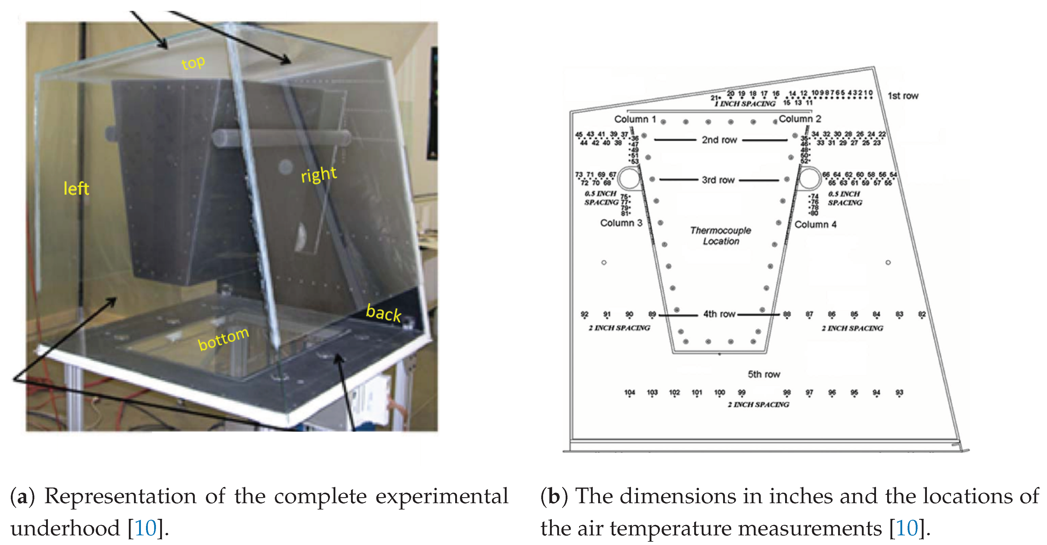
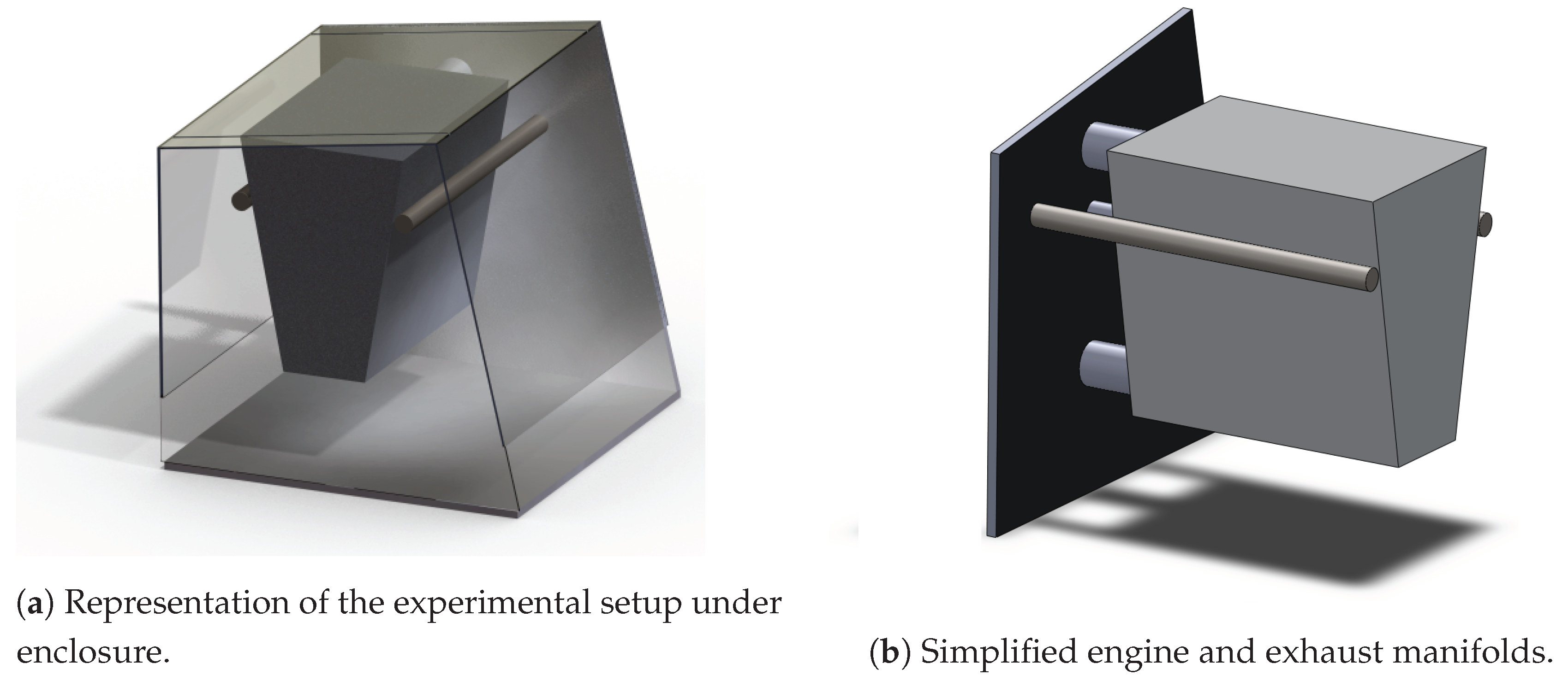
3. Physical Measurements

Physical experiments were performed by Merati et al. [10] and Chen et al. [9]. Their study provided detailed information about buoyancy-driven fluid flow and thermal phenonmena for a full-scale setup under both steady-state and transient conditions. These results were used for the validation purposes in the present paper. A brief decription of the experimental configuration that the numerical setup is based on, as well as the most relevant details of the experimental procedure, employed for the purpose of validation, are presented herein for completeness.

Experimental Setup and Procedure

The simple geometry was used in the physical experiments [9,10] to represent a typical vehicle underhood. Figure 1 illustrates the complete underhood that consists of two exhaust manifolds (represented by two cylindrical pipes), the engine block (represented by a trapezoidal prism) and the trapezoidal glass enclosure, which are the most relevant components to capture the temperature range during thermal soak.

The experiment replicated the thermal process governed by buoyancy-driven flow and heat transfer. The surface temperature of the exhaust manifolds was controlled at 600 ${}^{\circ }$C with inbuilt electrical heaters. Meanwhile the engine walls were cooled by internal water jet system, ensuring that the temperature of the engine is close to 100 ${}^{\circ }$C. It was determined that the heaters, mounted in the exhaust manifolds, dissipated approximately 2500 W of heat each, which corresponds to a heat flux of 31 kW/m${}^2$. These conditions were maintained constant until readings from temperature sensors mounted on the walls of the simplified engine stabilized, indicating steady heat fluxes. At this situation of steady-state heat transfer, surface temperature measurements were obtained on all solids. The location of the thermocouples used for these measurements is given in Section 4.2. After performing the steady temperature measurements, all heat and cooling sources were shut down and transient cool-down was started. Surface temperatures of all solid parts in the setup were measured for a period of 35 min after shutdown.

4. Numerical Procedure

4.1. Computational Domain

The computational domain illustrated in Figure 2 is an exact replica of the experimental setup, comprising the solid subdomain parts (the engine, the exhaust manifolds, and the enclosure), and the fluid subdomain (the volume under the enclosure, as well as the surrounding containment area), making it possible to employ the most suitable models for the fluid and solid parts, respectively, and to establish a direct coupling between these models. In this manner, the physics of the system can be capured with sufficient accuracy at lower computational costs.

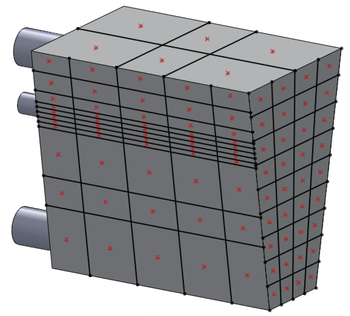
4.2. 1D Model of Transient Heat Transfer in Engine Solids

The 1D thermal model of heat transfer in the engine solids is used where the simplified engine and the exhaust manifolds are represented by lumped thermal masses. The concept of lumped thermal masses is based on the assumption that temperature variations within a solid, participating in heat transfer with a surrounding medium, can be neglected as compared to the temperature difference between the solid and the fluid. Previous experimental and numerical results have shown that this approach is valid for the exhaust manifolds and for all engine surfaces except the right and left engine walls, see Merati et al. [10] and Chen et al. [9] for more details. A good example of solids which can be accurately modeled using a single lumped thermal mass are the exhaust manifolds, for which experimental observations confirmed negligible internal temperature differences and uniform temperature distribution on their surfaces. The surfaces of the left and right engine walls, on the other hand, exhibit significant temperature gradients due to high radiative heat flux from the adjacent exhaust manifolds. Therefore, each of the engine side walls is represented by a network of 55 interfaced lumped thermal masses to provide sufficient spatial discretization to accurately capture the temperature distribution. The specific topography and dimensions of the thermal masses comprising this network are chosen so that their centers coincide with the locations of the thermocouples from the experiment, as illustrated in Figure 3. The actual materials used to build the parts of the experimental setup and their exact masses are used to model the lumped thermal masses. The variations of thermal conductivity and specific heat with temperature are accounted for. All relevant details are provided in

Table 2. Properties of thermal masses used to represent the simplified engine and the exhaust manifolds.

Material	Part	Number of Units	Mass (g)
Aluminum	Engine side wall	5	137
		5	132
		5	82
		25	35
		5	347
		5	209
		5	450
	Engine top	1	5796
	Engine bottom	1	2884
	Engine front	1	2939
	Engine back	1	2939
Steel	Exhaust manifold	1	6750

and

Table 3. Variations of $k_c$ and $c_p$ with T for aluminum and steel.

	Thermal Conductivity (W/m·K)		Specific Heat (J/kg·K)
T (C${}^{\circ }$)	Aluminum	Steel	Aluminum	Steel
27	237	60.5	903	434
127	240	56.7	949	487
327	231	48	1033	559
527	216	39.2	1146	685

, respectively. It should be noted that each row of interfaced thermal masses in the network representing the engine side wall corresponds to one row of adjacent sectors of the physical wall from top to bottom.

4.3. 3D CFD Numerical Solver for the Fluid Flow and Heat Transfer

The governing equations of the fluid flow are numerically solved in STAR-CCM+ and a polyhedral computational mesh with a total cell count of 25 million is generated from the CAD model of the enclosure and the containment area [4]. The average spatial discretization varies within the limits of 2 and 120 mm depending on the location. Denser mesh is used in the vicinity of the exhaust manifolds and in the upper part of the enclosure to more accurately resolve the temperature gradients and the buoyancy-driven flow field. The maximum cell size is 3 mm for all the surfaces located above the exhaust manifolds. The thickness of the first prismatic layer on the surfaces is approximately 0.3 mm, which results in maximum $y^{+}$ values of close to unity. Figure 4 illustrates the computational grid at the central section plane through the fluid domain. The boundary conditions for the 3D CFD model are the temperatures of the exhaust manifolds, the engine walls and the containment walls as obtained from stable measurement readings in the experiment [10]. A no-slip boundary condition is applied on all walls. An initially quiescent flow field with a uniform temperature of 30 ${}^{\circ }$C is considered. A second-order spatial discretization scheme is used with a coupled implicit solver [19] to compute the flow and temperature fields.

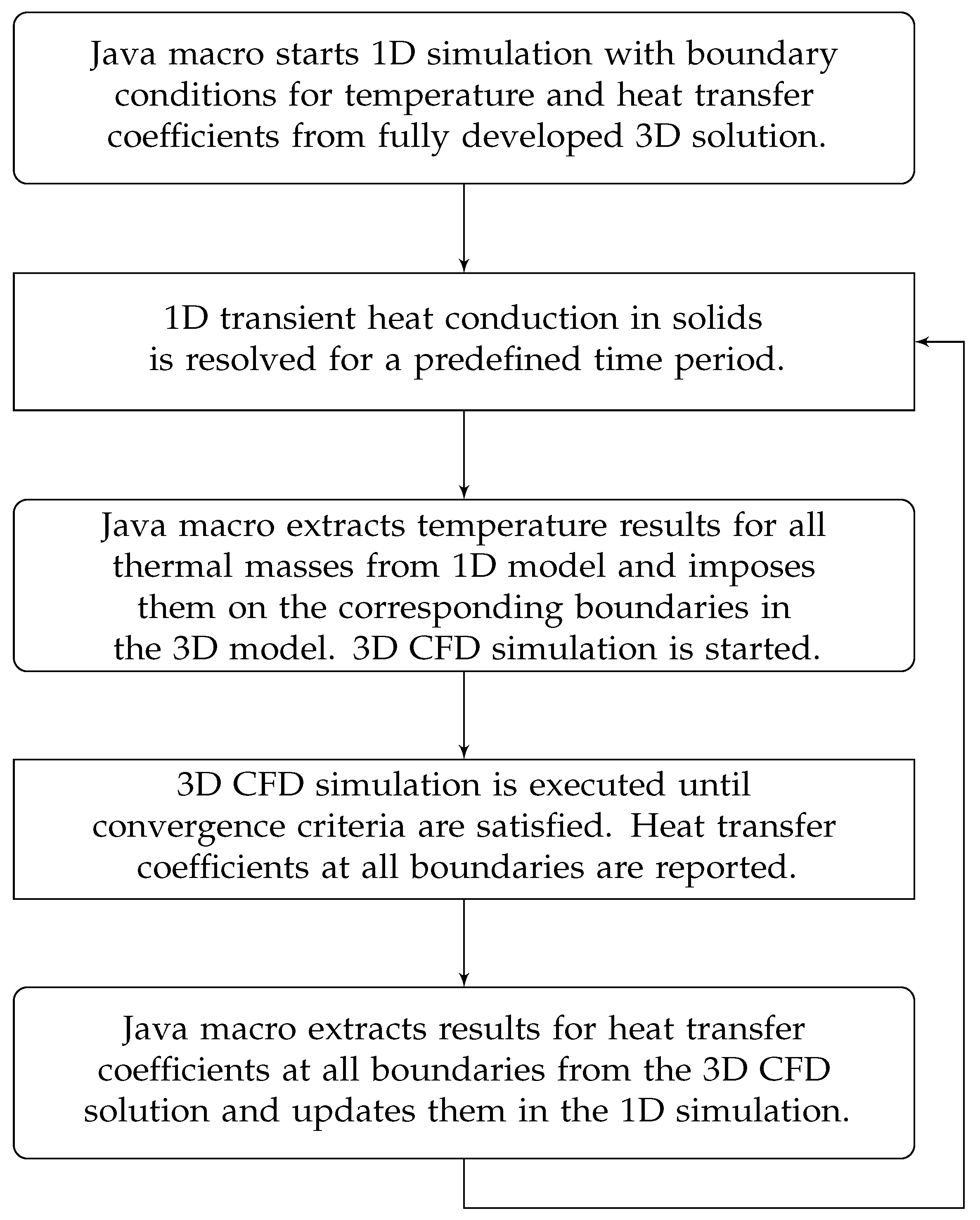
4.4. Description of 1D–3D Direct Coupled Approach

The computational procedure is initiated from the fully developed 3D solution of the flow and temperature fields using the surface temperature boundary conditions that correspond to the stable experimental measurements. The surface temperature of the exhaust manifolds was set to 600 ${}^{\circ }$C and the measured temperature distribution for the engine walls was imposed in the simulation. The resulting boundary heat transfer and averaged fluid temperatures at boundary cells from the steady-state 3D flow simulation are used as boundary conditions for the transient 1D thermal analysis in the solid domain to compute the wall surface temperature. The transient simulation of heat transfer in the solids is consequently initiated using temperature settings for the thermal masses that correspond to the exact temperature distribution measured in the beginning of the experimental cool-down. The 1D transient simulation of heat transfer in the solids is run for constant time step. In the end of this time period the temperatures of each thermal mass are sent to the 3D CFD model. The updated wall temperature is then used as a new boundary condition in the next iteration of the 3D CFD simulation. This iterative coupling procedure is implemented as a Java macro and is presented as a flow chart in Figure 5. The procedure lasts for a specified duration of the cool-down period. The data exchange between 1D and 3D simulations takes place at a predefined time interval that is referred to as time interval between simulation exchanges. As the presented computational approach employs a transient thermal analysis in the solid domain and a steady-state analysis of the flow field in the fluid domain, it is referred to as quasi-transient. The steady-state simulations capture the features of the fluid flow with sufficient accuracy, while keeping the computational costs sufficiently low to allow for fast transient simulations of long periods of engine cool-down.

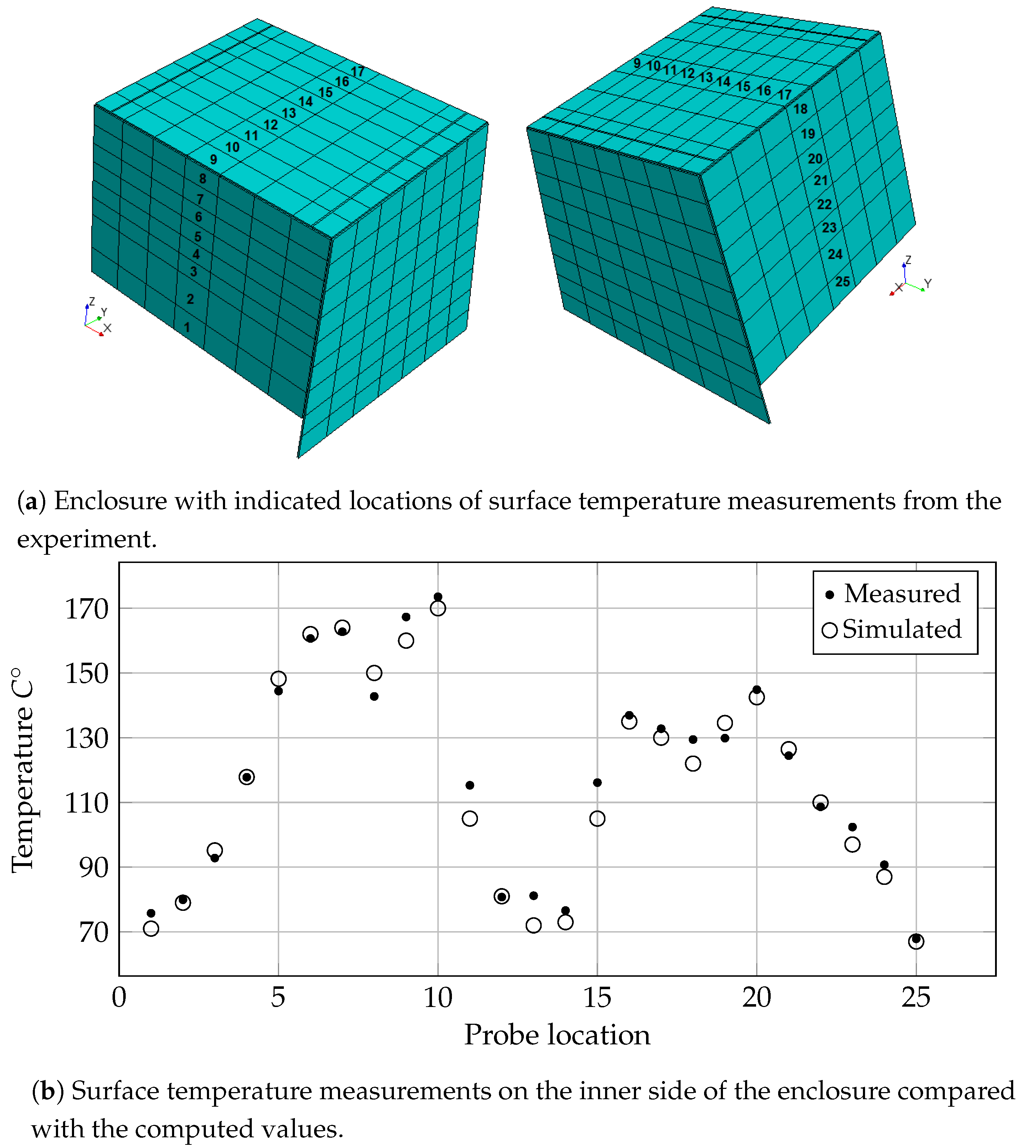
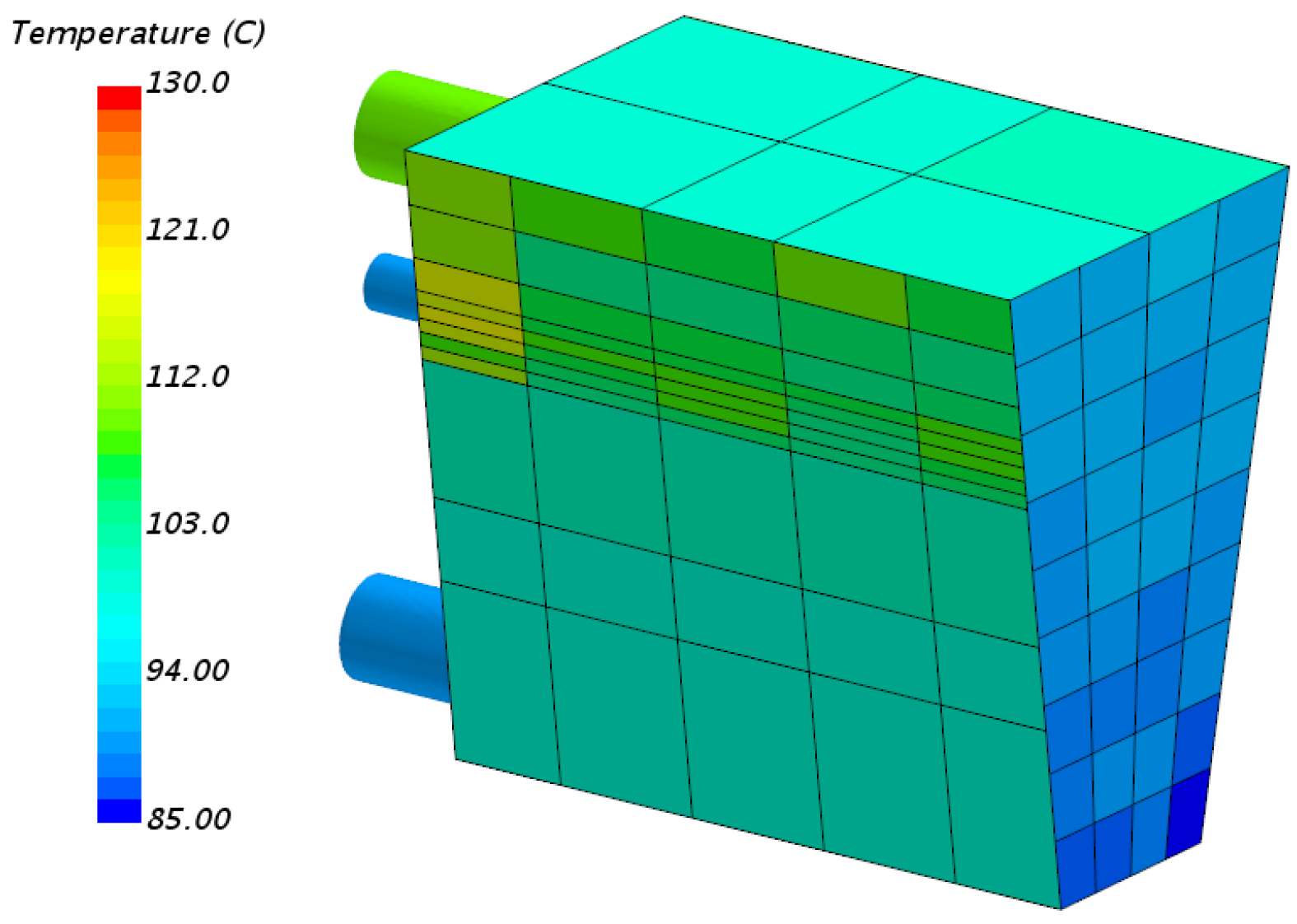
4.5. Results from Simulations of Steady-State Heat Transfer

The steady-state heat transfer, confirmed by the stable temperature readings during the initial part of the experiment, was first replicated in a standalone 3D CFD solver without any coupling to the 1D model. The temperature boundary conditions for the engine and the exhaust manifolds, see Figure 6, correspond to experimental measurements obtained from surface-mounted thermocouples with locations previously shown in Figure 3.

Furthermore, the temperature of the inner side of the glass enclosure along the traverse central section plane (see Figure 7) is strongly affected by the radiation heat from the exhaust manifolds. Due to lack of any measured emissivity coefficients, these parameters are calibrated to achieve optimal correlation between the computed and experimentally measured results for the surface temperature on the inside of the glass enclosure. The iterative calibration procedure used different values for the emissivity coefficients of the exhaust manifolds and engine walls. These coefficients were chosen to achieve optimal predictions of the surface temperatures on the inside of the enclosure in proximity to the exhaust manifolds, as shown in Figure 7b. The obtained values for the emissivity of the exhaust manifolds and engine block are 0.75 and 0.5, respectively, and correspond to documented values of similar materials.

5. Results and Discusssion

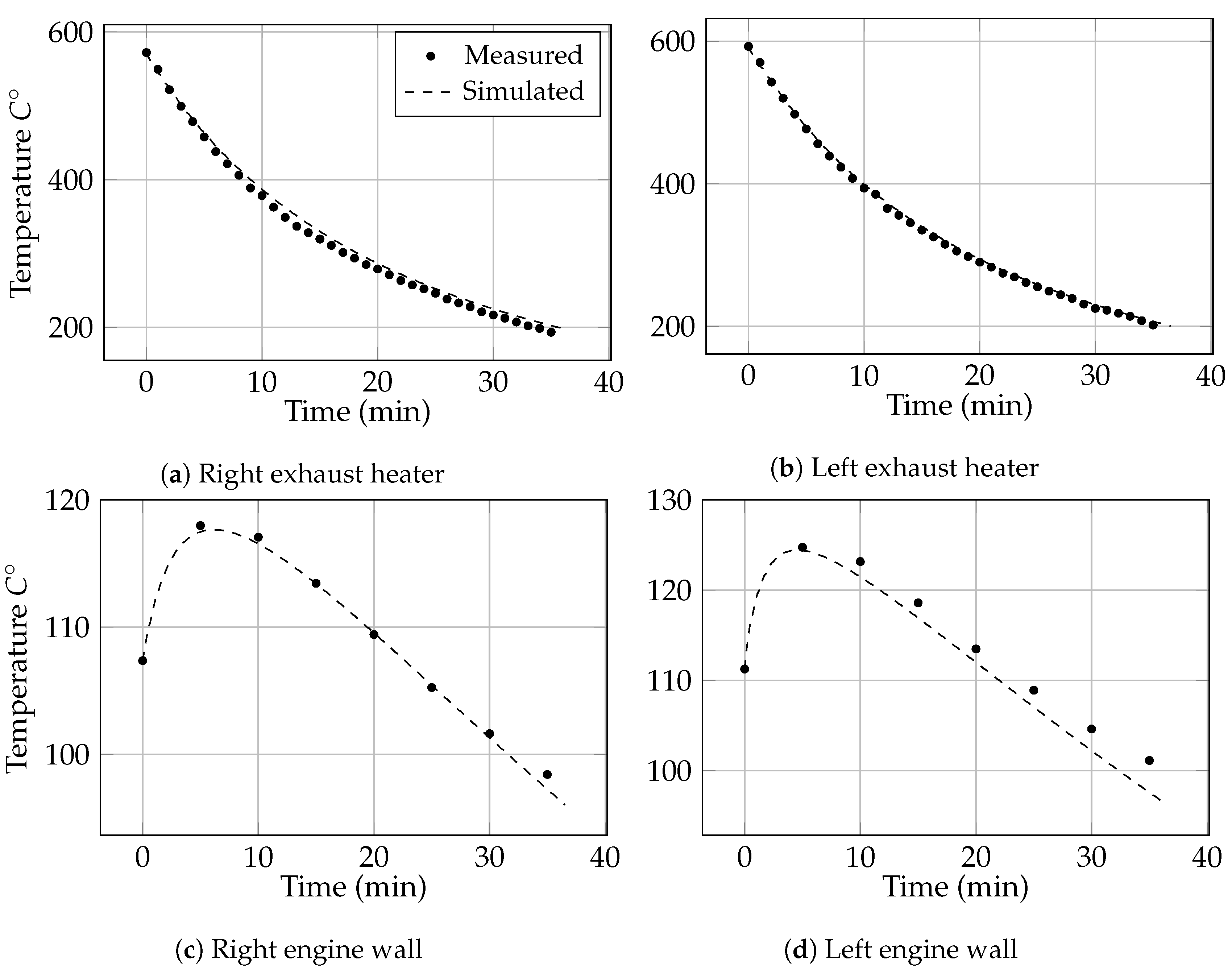
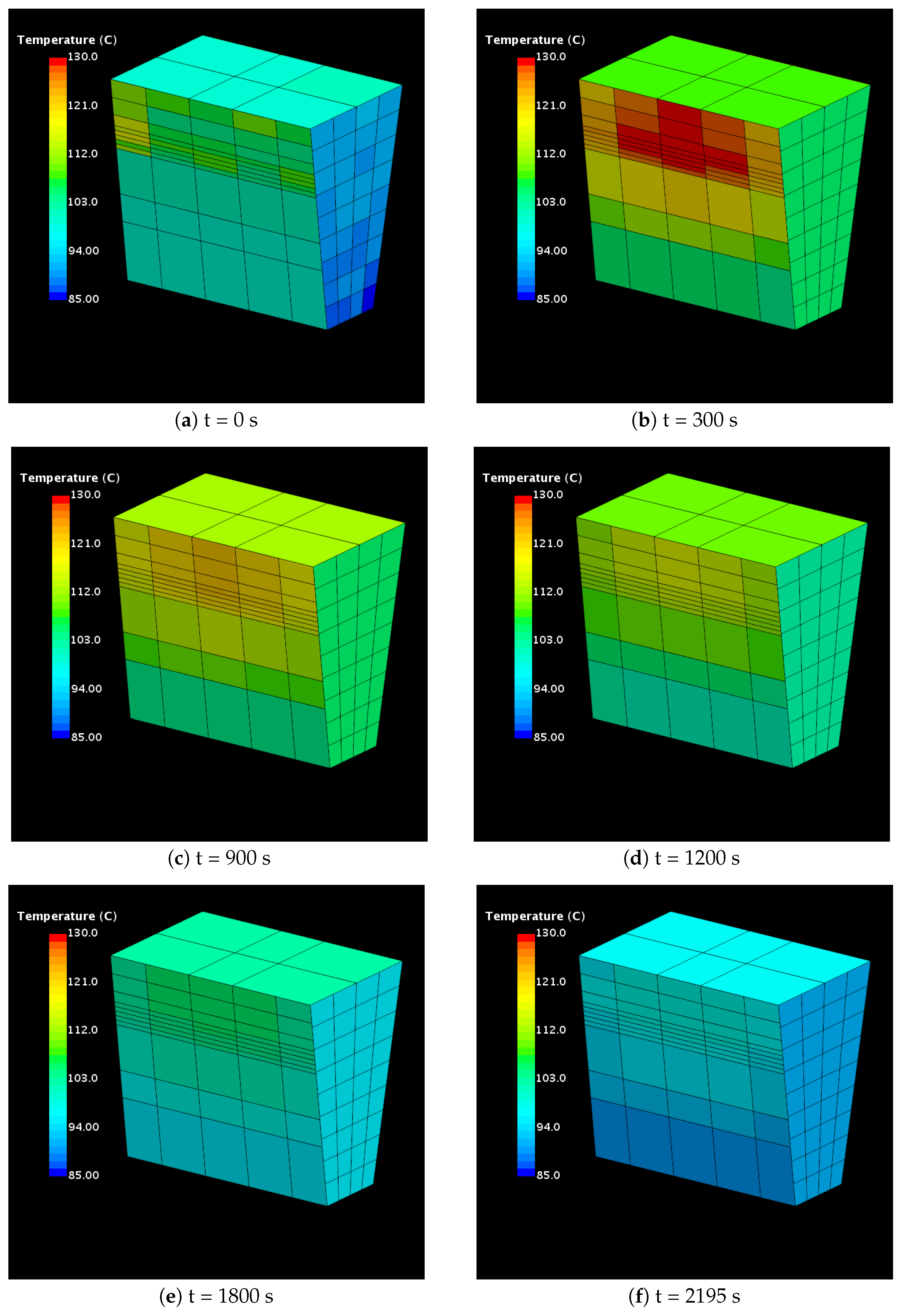
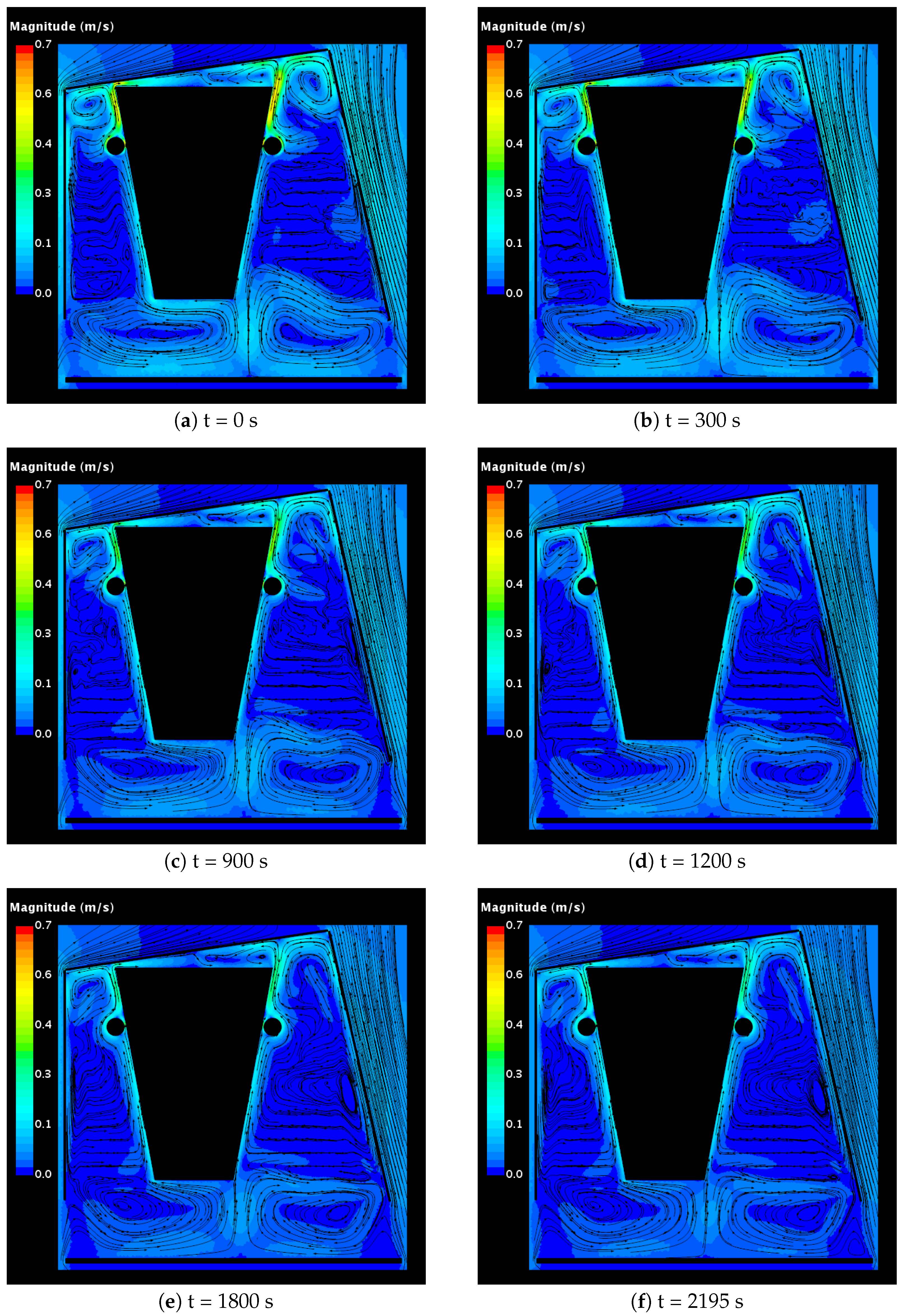
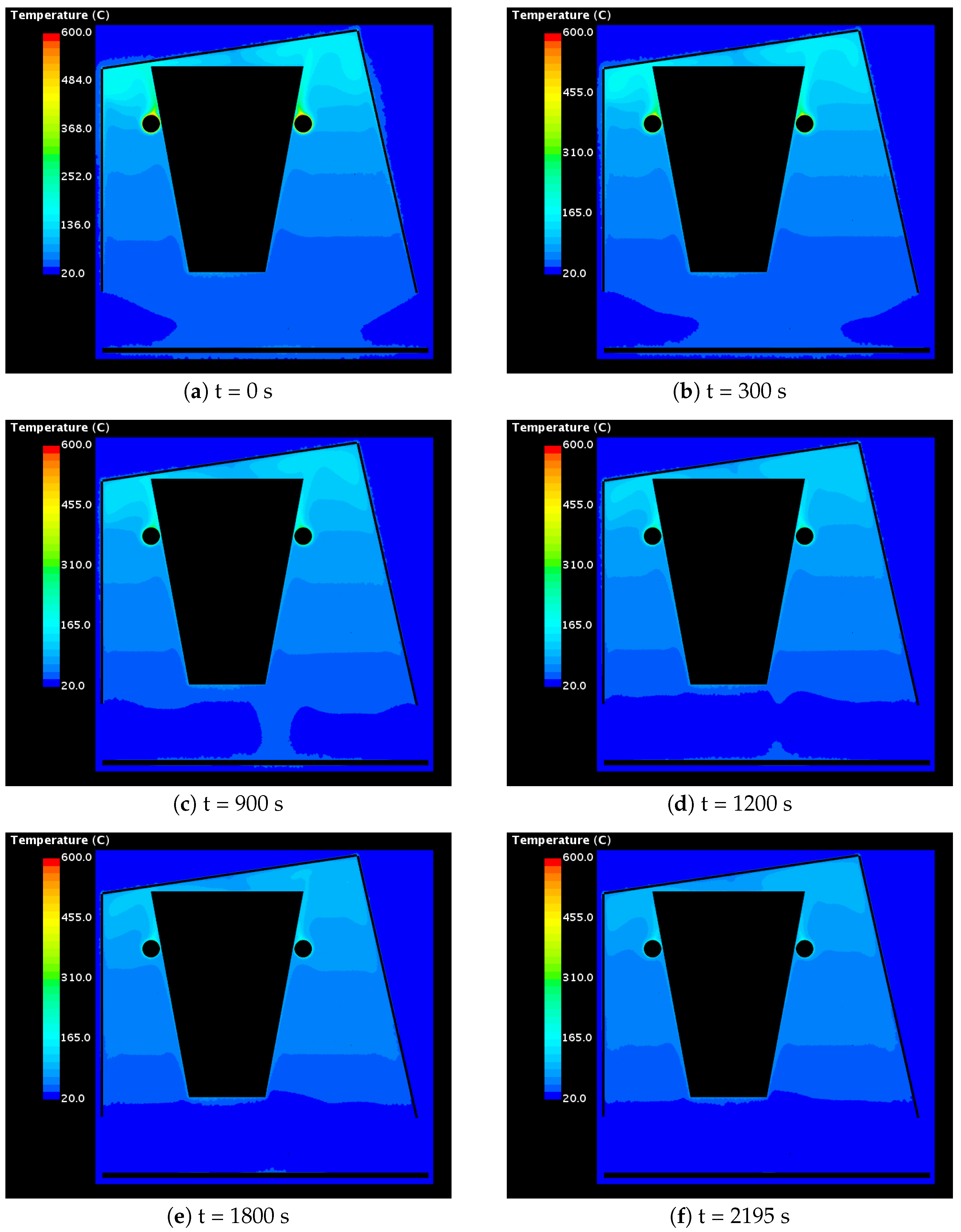
Results from Simulations of Transient Cool-Down

A coupled 1D–3D simulation is carried out to predict the temperature development in the engine solids during the thermal soak and cool-down period after turning off the heating and cooling systems. The coupled simulation is initiated from a fully developed solution of steady-state heat transfer. Given that the resulting heat transfer and averaged fluid temperatures in the boundary cells from the CFD simulations are repeatedly updated in the continuous thermal simulation in the solid domain at certain time interval, it was necessary to first perform sensitivity analysis to determine the effects of this time interval for 1D–3D data exchange on the accuracy of the temperature prediction. For that purpose, the surface temperature was predicted for four different exchange intervals of 2, 5, 10 and 15 s, respectively. The relationship between the accuracy and the exchange interval duration is shown in Figure 8a. It is seen that the percentage difference between the simulated and measured values increases significantly as the time interval decreases from 15 to 5 s. Since a marginal improvement in the accuracy is observed for the exchange intervals shorter than 5 s, accompanied by a notable increase in the computational time (see Figure 8b), it was decided that the data exchange between 1D and 3D computations should take place every 5 s.

The coupled simulation predicts the temperature development in each thermal mass. The temperature distribution across the surfaces of the engine at six different time instances is presented in Figure 9. The effect of thermal soak on the engine wall surface temperature is evident from Figure 9a,b. Heat dissipated by the exhaust manifolds during the initial 300 s is absorbed by the adjacent engine walls through conductive, convective and radiative heat transfer, resulting in overall increase in the temperature of the engine.

Furthermore, the time history of the velocity and temperature fields in the central section plane is presented, see Figure 10 and Figure 11, respectively. In Figure 10a the most prominent flow structures are two pairs of counter-rotating vortexes, powered by the rising hot plumes above the exhaust manifolds and one more pair of large counter-rotating vortexes in the bottom of the enclosure near the side openings. While their velocity magnitudes decay over time, these flow structures remain present over the entire course of the cool-down period.

Figure 12 presents the development of the average surface temperature of the engine walls and the exhaust manifolds during the cool-down cycle of 35 min. The results from the actual experimental study are included for the purpose of validation. A very good agreement between the computed and measured temperature results is seen for both exhaust manifolds and the right engine wall. The surface temperature of the left engine wall is underpredicted by approximately 3% as compared to the experimental results. This discrepancy is attributed to the fact that the simulations do not accurately account for the presence of the gaskets that are used to seal the adjacent metal plates that comprise the simplified engine. The error of the prediction can thus be reduced by introducing additional thermal resistances between the solid interfaces, however no experimental data for these is available.

6. Concluding Remarks

This work presents a direct coupled 1D–3D quasi-transient computational approach to compute the continuous development of temperatures of solids in a simplified engine bay during thermal soak and cool-down period. The computational domain represents a simplified full scale underhood geometry from an actual experiment, consisting of a simplified engine and two cylindrical exhaust manifolds covered by an open enclosure and placed in a containment room. A transient 1D thermal analysis is carried out in the engine solids, while coupled steady-state 3D computations predict the flow field. The heat transfer analysis accounts for heat conduction, convective heat transfer and thermal radiation. The coupling between 1D and 3D simulations is achieved by imposing heat transfer coefficients and averaged fluid temperatures in the boundary cells from the CFD simulations as input data for 1D analysis that calculates temperature of the solid surfaces, which are then used as new boundary conditions in the next iteration of the 3D CFD simulation.

The numerical simulations predict the average surface temperature of the engine block and the exhaust manifolds during the thermal soak and cool-down period. The computed temperature values are in very close agreement with the experimentally measured data. A minor discrepancy in the computed results for the average temperature of the left engine wall is attributed to the fact that the simulations neglect the thermal resistances of the gaskets that are present in the physical setup and that the model assumed zero thermal resistance between the interfaced solids. By introducing additional thermal resistances it is possible to increase the prediction accuracy.

The validation results presented herein demonstrate the feasibility of the direct coupled 1D–3D computational approach to predict the effects of buoyancy-driven heat transfer on the surface temperature of the engine solids during thermal soak and cool-down events. This work deepens the understanding of the coupled numerical procedure to analyze underhood heat transfer essential for design and optimization of future vehicle thermal management solutions.

References

1. Lu, P.; Gao, Q.; Liang, L.; Xue, X.; Wang, Y. Numerical Calculation Method of Model Predictive Control for Integrated Vehicle Thermal Management Based on Underhood Coupling Thermal Transmission. Energies 2019, 12, 259. [Google Scholar] [CrossRef]
2. Wang, Y.; Gao, Q.; Zhang, T.; Wang, G.; Jiang, Z.; Li, Y. Advances in integrated vehicle thermal management and numerical simulation. Energies 2017, 10, 1636. [Google Scholar] [CrossRef]
3. Muscio, A.; Mattarelli, E. Potential of Thermal Engine Encapsulation on Automotive Diesel Engines; SAE Technical Paper; SAE International: Detroit, MI, USA, 2005. [Google Scholar] [CrossRef]
4. Minovski, B.; Lofdahl, L.; Gullberg, P. Numerical Investigation of Natural Convection in a Simplified Engine Bay; SAE Technical Paper; SAE International: Detroit, MI, USA, 2016. [Google Scholar] [CrossRef]
5. Sweetman, B.; Schmitz, I.; Hupertz, B.; Shaw, N. Numerical Investigation of Vehicle Drive and Thermal Soak Conditions in a Simplified Engine Bay. SAE Int. J. Passeng. Cars Mech. Syst. 2017, 10, 433–445. [Google Scholar] [CrossRef]
6. Franchetta, M.; Suen, K.; Williams, P.; Bancroft, T. Investigation into Natural Convection in an Underhood Model Under Heat Soak Condition; SAE Technical Paper 2005-01-1384; SAE International: Detroit, MI, USA, 2005. [Google Scholar] [CrossRef]
7. Franchetta, M.; Bancroft, T.; Suen, K. Fast Transient Simulations of Vehicle Underhood in Heat Soak; SAE Technical Paper 2006-01-1606; SAE International: Detroit, MI, USA, 2006. [Google Scholar] [CrossRef]
8. Davis, C. Investigation of Underhood Buoyancy driven Flow and Thermal Measurements in a Simplified Full Scale Underhood Engine Compartment with Open Enclosure. Master’s Thesis, Western Michigan University, Kalamazoo, MI, USA, 2009. [Google Scholar]
9. Chen, K.; Johnson, J.; Merati, P.; Davis, C. Numerical Investigation of Buoyancy-Driven Flow in a Simplified Underhood with open Enclosure. SAE Int. J. Passeng. Cars Mech. Syst. 2013, 6. [Google Scholar] [CrossRef]
10. Merati, P.; Davis, C.; Chen, K.H.; Johnson, J.P. Underhood Buoyancy Driven Flow—An Experimental Study. J. Heat Transf. 2011, 133, 1–9. [Google Scholar] [CrossRef]
11. Yuan, R.; Sivasankaran, S.; Dutta, N.; Jansen, W.; Ebrahimi, K. Numerical investigation of buoyancy-driven heat transfer within engine bay environment during thermal soak. Appl. Therm. Eng. 2019, 164, 114525. [Google Scholar] [CrossRef]
12. Truitt, R. Fundamentals of Aerodynamic Heating; Ronald Press Co.: New York, NY, USA, 1960. [Google Scholar]
13. Wilcox, D.C. Turbulence Modeling for CFD, 2nd ed.; DCW Industries: La Canada, CA, USA, 2006. [Google Scholar]
14. Incropera, F.P.; Dewitt, D.P.; Bergman, T.L.; Lavine, A.S. Fundamentals of Heat and Mass Transfer; John Wiley and Sons: New York, NY, USA, 2007. [Google Scholar]
15. Lauriat, G.; Desrayaud, G. Effect of surface radiation on conjugate natural convection in partially open enclosures. Int. J. Therm. Sci. 2005, 45, 335–346. [Google Scholar] [CrossRef]
16. Miroshnichenko, I.V.; Sheremet, M.A.; Mohamad, A.A. Numerical simulation of a conjugate turbulent natural convection combined with surface thermal radiation in an enclosure with a heat source. Int. J. Therm. Sci. 2016, 109, 172–181. [Google Scholar] [CrossRef]
17. Modest, M.F. Radiative Heat Transfer, Series in Mechanical Engineering; McGraw-Hill: New York, NY, USA, 1993. [Google Scholar]
18. Siegel, R. Thermal Radiation Heat Transfer; Hemisphere Pub. Corp: Washington, DC, USA, 1992. [Google Scholar]
19. StarCCM+ User Guide v.11.04. Available online: http://www.cd-adapco.com/products/star-ccm/documentation (accessed on 26 August 2019).
Figure 1. Experimental setup [10].
Energies 12 04156 g001
Figure 2. CAD model of the experimental setup.
Energies 12 04156 g002
Figure 3. The simplified engine with indicated locations of thermocouples from the experiment.
Energies 12 04156 g003
Figure 4. Computational grid in the central section plane in proximity to the enclosure. Note that only the part of the containment room in the vicinity of the enclosure is seen. The white areas belong to the solid domain and represent the engine block and the exhaust manifolds.
Energies 12 04156 g004
Figure 5. Flow chart describing the coupling procedure between 1D and 3D models.
Energies 12 04156 g005
Figure 6. Boundary condition for temperature distribution across the engine surfaces used in the standalone CFD simulation. The presented temperature distribution is obtained from measurements during steady mode of heat transfer.
Energies 12 04156 g006
Figure 7. Experimentally and computationally determined temperatures of the enclosure.
Energies 12 04156 g007
Figure 8. Sensitivity study of the effect of update frequency on the accuracy and speed of the simulations.
Energies 12 04156 g008
Figure 9. Simulation results for the temperature of the engine walls.
Energies 12 04156 g009
Figure 10. Simulation results for the velocity field in the central section plane.
Energies 12 04156 g010
Figure 11. Simulation results for the temperature of the fluid in the central section plane.
Energies 12 04156 g011
Figure 12. Comparison between the computed and experimentally measured average surface temperatures of the engine solids during cool-down.
Energies 12 04156 g012