Article

Solar Power Interval Prediction via Lower and Upper Bound Estimation with a New Model Initialization Approach

1
State Grid Zhejiang Electrical Power Research Institute, Hangzhou 310014, China
2
School of Electrical Engineering, Southeast University, Nanjing 211189, China
*
Author to whom correspondence should be addressed.
Energies 2019, 12(21), 4146; https://doi.org/10.3390/en12214146
Submission received: 29 September 2019 / Revised: 26 October 2019 / Accepted: 28 October 2019 / Published: 30 October 2019
(This article belongs to the Special Issue Ensemble Forecasting Applied to Power Systems)

Abstract

:
This paper proposes a new model initialization approach for solar power prediction interval based on the lower and upper bound estimation (LUBE) structure. The linear regression interval estimation (LRIE) was first used to initialize the prediction interval and the extreme learning machine auto encoder (ELM-AE) is then employed to initialize the input weight matrix of the LUBE. Based on the initialized prediction interval and input weight matrix, the output weight matrix of the LUBE could be obtained, which was close to optimal values. The heuristic algorithm was employed to train the LUBE prediction model due to the invalidation of the traditional training approach. The proposed model initialization approach was compared with the point prediction initialization and random initialization approaches. To validate its performance, four heuristic algorithms, including particle swarm optimization (PSO), simulated annealing (SA), harmony search (HS), and differential evolution (DE), were introduced. Based on the experiment results, the proposed model initialization approach with different heuristic algorithms was better than the point prediction initialization and random initialization approaches. The PSO can obtain the best efficiency and effectiveness of the optimal solution searching in four heuristic algorithms. Besides, the ELM-AE can weaken the over-fitting phenomenon of the training model, which is brought in by the heuristic algorithm, and guarantee the model stable output.

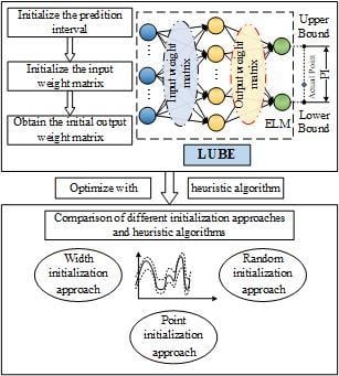
Graphical Abstract

1. Introduction

With the increasing global energy consumption, renewable energy and its application technologies have received extensive attention and are being studied enthusiastically. The intermittent nature and volatility of renewable energy, as significant factors, restrict its exploitation and penetration. An accurate forecast is required to guarantee the stability and economy of power systems. However, the randomness and indeterminacy of natural resources bring great difficulties for solar power predictions.
Traditional solar power point prediction provides limited forecast information, which causes risk [1]. Solar power interval prediction offering interval information under a certain confidence level breaks a new pathway to handle forecasting uncertainty. The interval prediction technology aims at predicting a narrow interval, encompassing as many predicted points as possible. The high-quality prediction intervals are of benefit to static safety analysis and risk evaluation in power systems. However, solar power interval prediction attracts less attention compared to point prediction. The existing prominent interval prediction methods include the statistical method and data-driven method.
The statistical methods are first employed to construct the prediction interval. Statistical methods usually require prior knowledge or distribution assumption of forecasting errors [2,3,4,5]. They often assume that the forecast errors follow a normal distribution with a zero mean or t-student distribution [6]. The bootstrap [7], Bayesian [8], mean-variance estimation [5], and delta methods [9] are the four prominent and traditional methods. These four methods were analyzed from calculations, interval precision, and interval width, which revealed that each method had its shortcomings [10]. The prediction errors display different characters and differ in various application fields. Thus, it is important to make the appropriate distribution assumption, which might result in poor forecasting performance. Li et al. acquired a precise distribution characteristic based on the divided dataset by the envelope-based clustering algorithm. There are also several statistical methods without any prior assumption for probabilistic prediction, such as kernel density estimation [11], ensemble simulations [12], and quantile regression [3].
Data-driven methods are gradually introduced to avoid distribution assumptions. The lower and upper bound estimation (LUBE) structure for interval prediction was first developed by Khosravi et al. [13]. Two output units of the neural network (NN) model were employed to represent the upper and lower bounds of the predicted interval. Such nonparametric models are further widely utilized in many research works [14,15,16]. In the process of training the LUBE, two prominent evaluation metrics, coverage probability and interval width, are considered. Due to their contradictoriness, the LUBE training can be considered as a multi-objective or single-objective optimization model [17,18,19]. In [20], a new multi-objective optimization method using multi-objective swarm algorithm was proposed to adjust the machine learning model, which revealed superior forecasting performance to the single-objective one. In [21], the Pareto optimal solutions were used to construct a multi-objective framework and Pareto solutions obtained an ensemble of optimal solutions. Due to the discontinuous differentiability of the cost function, it is hard to train the NN through the traditional analytical algorithm. Heuristic algorithms such as particle swarm optimization (PSO) and simulated annealing (SA) are employed in this situation.
Most previous interval prediction methods based on LUBE models concentrate on the building of optimization objective and the selection of intelligent algorithms. The initialization method of the NN parameters is rarely studied. However, the initial solution of heuristic algorithms significantly affects their evolution process and performance.
ELM-AE employed in this paper aims at enhancing the generalization capability of the forecasting model. Besides this, current application objects of interval prediction mainly include wind speed, wind power, electricity load, and electricity price prediction. Solar energy, as a representative renewable resource, also deserves some discussion for interval prediction.
This paper proposes a new model initialization approach for the prediction interval based on the LUBE structure. The ELM-AE is first utilized to initialize the input weight matrix of the LUBE model and the linear regression interval estimation (LRIE) is then used to initialize the prediction interval. The initial prediction interval obtained by LRIE is then employed to update the initial parameters of the LUBE model. Numerous comparison experiments are conducted to validate the performance of the proposed model initialization approach.
Some experiments using the proposed initialization approach, traditional initialization approach, and random initialization approach are implemented with the same sample data. Different heuristic algorithms, including particle swarm optimization (PSO), simulated annealing (SA), harmony search (HS), and differential evolution (DE), are conducted to evaluate the impact of the initial solution on different heuristic algorithms.
The remainder of this paper is organized as follows. Section 2 introduces the LUBE method employing ELM and two primary evaluation indices of forecasting intervals. The proposed model initialization approach is described in Section 3. Experiments and results are reviewed in Section 4. Finally, Section 5 makes some conclusions of this work and discusses some guidelines for future work.

2. Lower and Upper Bound Estimation

The LUBE method utilizing the neural network structure has been widely used to estimate the prediction interval. The schematic diagram of the LUBE method is shown in Figure 1. The ELM with two output nodes is regarded as the prediction model of LUBE. The output of the two output nodes represents the predicted upper and lower bound. Because the actual predicted interval is unknown and uncertain, the traditional background propagation algorithm cannot be used to train the ELM. The training of the ELM is converted to a parameter optimization problem and the heuristic algorithm is utilized to obtain the optimal parameters of the LUBE.

2.1. ELM

The ELM introduced by Huang, et al. [22] is a single-hidden layer feed forward neural network with excellent generalization performance and fast learning speed. Thus, the ELM is utilized as the prediction model in this work. In Figure 1, the ELM only has three layers, the input layer, hidden layer, and output layer. Two neuron units in the output layer separately represent the upper and lower bounds of the predicted interval.
In the normal ELM model, suppose that N samples { x j , t j } j = 1 N are given, where xj Rn, representing the input vector, tj Rm, representing the target vector. The input data are transmitted to the L dimensional feature space constructed by the hidden layer and the output element of the network is obtained by Equation (1):
f L ( x ) = i = 1 L β i h i ( x ) = h ( x ) β
where h(x) indicates the outputs of hidden neuron node and the L element corresponds to the outputs of L hidden nodes generated from activation function. Likewise, β = [β1, …, βL]T is the output weight matrix. The goal of the single hidden layer neural network is to minimize the error between the output value and the actual quantity. In matrix form, the target of the network is achieved by Equation (2):
H β = T
where H = [hT(x1), …, hT(xN)]T and T = [t1, …, tN ]T. Thus, in ELM, the output weight β can be expressed as Equation (3):
β ^ = H T
where H is the Moore–Penrose generalized inverse of matrix.

2.2. The Evaluation and Training of LUBE

To evaluate the prediction performance, the mean prediction interval width, PImean, and prediction interval coverage probability (PICP) in (4)–(5) are introduced. The PImean qualifies the width of prediction interval. The PICP indicates the percentage of the probability targets covered by the corresponding prediction intervals.
PI mean = 1 N i = 1 N ( t ¯ i t i _ )
PICP = 1 N i = 1 N 1 [ t i _ , t ¯ ] ( t i )
where t ¯ i and t i _ are the predicted upper and lower bounds of the dataset {(xi, ti), i = 1, …, N}. Since the forecasting interval width is strongly associated with the range of the targets, normalized width evaluation index is more suitable for intuitional comparison. A new normalized index, called prediction interval normalized root-mean-square width (PINRW), is employed as in (6) [14]:
PINRW = 1 R 1 N i = 1 N ( t ¯ i t i _ ) 2
where R is the range of the forecasting targets. In general, R is equal to the difference between the maximum and minimum values of the training set.
The PImean and PICP (or PINRW) are the contradictory indexes. An ideal interval aims to maximize PICP and minimize PImean simultaneously. However, a balance and a compromise are required in practice. The cost function coverage width-based criterion (CWC) is introduced to evaluate the predicted interval. The flexible index combines prediction interval coverage percentage and width simultaneously, which could evaluate the overall performance of the prediction intervals and guide the generation of intervals:
CWC = PINRW ( 1 + 1 [ 0 , δ ) ( PICP ) e η ( PICP δ ) )
where the hyper-parameter η magnifies the difference between PICP and δ, which should be a large value.
The training of LUBE can be regarded as an optimization problem. The minimization of CWC is the optimization objective and the output weight matrix of ELM is the independent variable. The heuristic algorithm is employed to obtain the optimal output weight matrix by minimizing CWC. The initialization of the output weight matrix can be generated randomly, called the random initialization (RI) approach. The output weight matrix obtained by the point prediction approach also can be utilized to initialize the output weight matrix of the LUBE, called the point initialization (PI) approach [13].

3. Proposed Model Initialization Approach

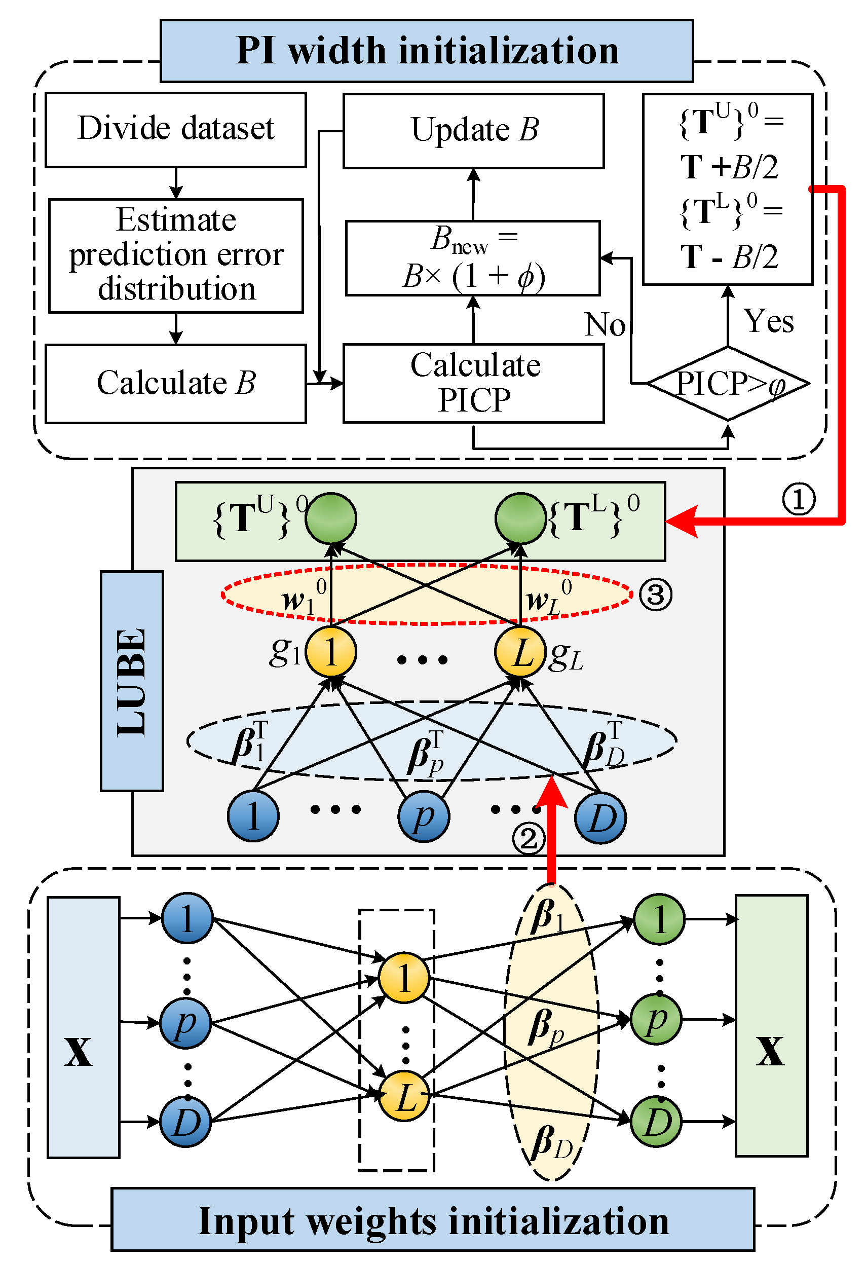
In the traditional LUBE interval prediction model, the random input weight matrix and search capacity of the heuristic algorithm significantly impact the final prediction performance. In this section, the proposed model initialization approach is introduced, including prediction interval initialization and input weight matrix initialization, shown in Figure 2. The initial prediction interval {TU, TL}0 was first obtained by the prediction interval width initialization method. The input weight matrix βT was then generated by the ELM-AE. The initial output weight matrix w0 was finally gained by training the LUBE prediction model based on the initial prediction interval and input weight matrix.

3.1. Prediction Interval Initialization

In order to initialize the interval width and estimate initial prediction interval value of the whole training dataset {TU, TL}0, cross-validation technology was utilized. In Figure 2, the training dataset {X, T} is first divided for cross validation. In each part, suppose T = + μ, E(μ) = 0 and Var(μ) = σ2I. Then, the prediction error e0 on a single future observation {X0, T0} follows the normal distribution e0 ~N(0, σ2(1+X0(XTX)−1X0T)) shown in (8) and (9):
E ( e 0 ) = E ( μ 0 X 0 ( ( X T X ) 1 X T ( X Φ + μ ) Φ ) ) = E ( μ 0 X 0 ( X T X ) 1 X T μ ) = 0
V a r ( e 0 ) = V a r ( μ 0 X 0 ( ( X T X ) 1 X T μ ) = σ 2 ( 1 X 0 ( X T X ) 1 X 0 T )
Therefore, the prediction interval is T 0 ± t α / 2 , n m σ ( 1 + X 0 ( X T X ) 1 X 0 T ) . According to (4), the initial interval width is B0.
The PImean of the {X, T} is then calculated as the initial interval width, denoted as B0. To guarantee the expected prediction interval coverage probability φ is satisfied, the B0 should be further adjusted through the binary search algorithm [18]. The actual value of the target T and the initial interval width B compose the initial prediction interval, {TU, TL}0, shown as (10):
{ T U } 0 = T + B / 2 , { T L } 0 = T B / 2
The details of prediction interval width initialization are presented in the following steps (see Algorithm 1):
Algorithm 1 Prediction Interval Width Initialization
Input:
Training data {X,T} = { ( x i , t i ) | x i ,   t i ,   i = 1 , 2 , , n } ;
Nominal confidence α;
Number of data subsets m;
Expected prediction interval coverage probability φ.
Output:
Initial Prediction Interval {TU, TL}0.
(a) Calculate initial interval width B0 of {X, T}.
(a-1) Divide the training dataset {X, T} into m subsets;
(a-2) Sequentially select one subset as the testing data and other subsets are regarded as the training data;
(a-3) Separately estimate the prediction error distribution and prediction interval of each test data according to α based on the corresponding training data.
(a-4) Calculate PImean by (4), denoted as B0.
(a-5) Calculate {TU, TL}0 by (10), where B = B0.
(b) Calculate the PICP of the ELM trained through {TU, TL}0 for the training set. If PICP < φ, go to (c). If PICP ≥ φ, output {TU, TL}0.
(c) Update B by the binary search algorithm
(c-1)Bnew = B× (1 + ϕ);
(c-2) Update {TU, TL}0 by (10) and go to (b), where B = Bnew;

3.2. Input Weight Matrix Initialization

In conventional training of the ELM model, its input weights are randomly generated. However, the random input weights have influence on the output weights training, which further impact the prediction performance, especially model training through the heuristic algorithm.
The ELM-AE is capable of learning a useful feature representation [23], which could improve the generalization of the predicted model via projecting the input data into a different dimensional space [24]. ELM-AE has shown good capacity to learn a useful feature representation. The unique differentiation of the specific input data is reduced by the feature transformation. The generalization of the predicted model will be improved via projecting the input data into a different dimensional space.
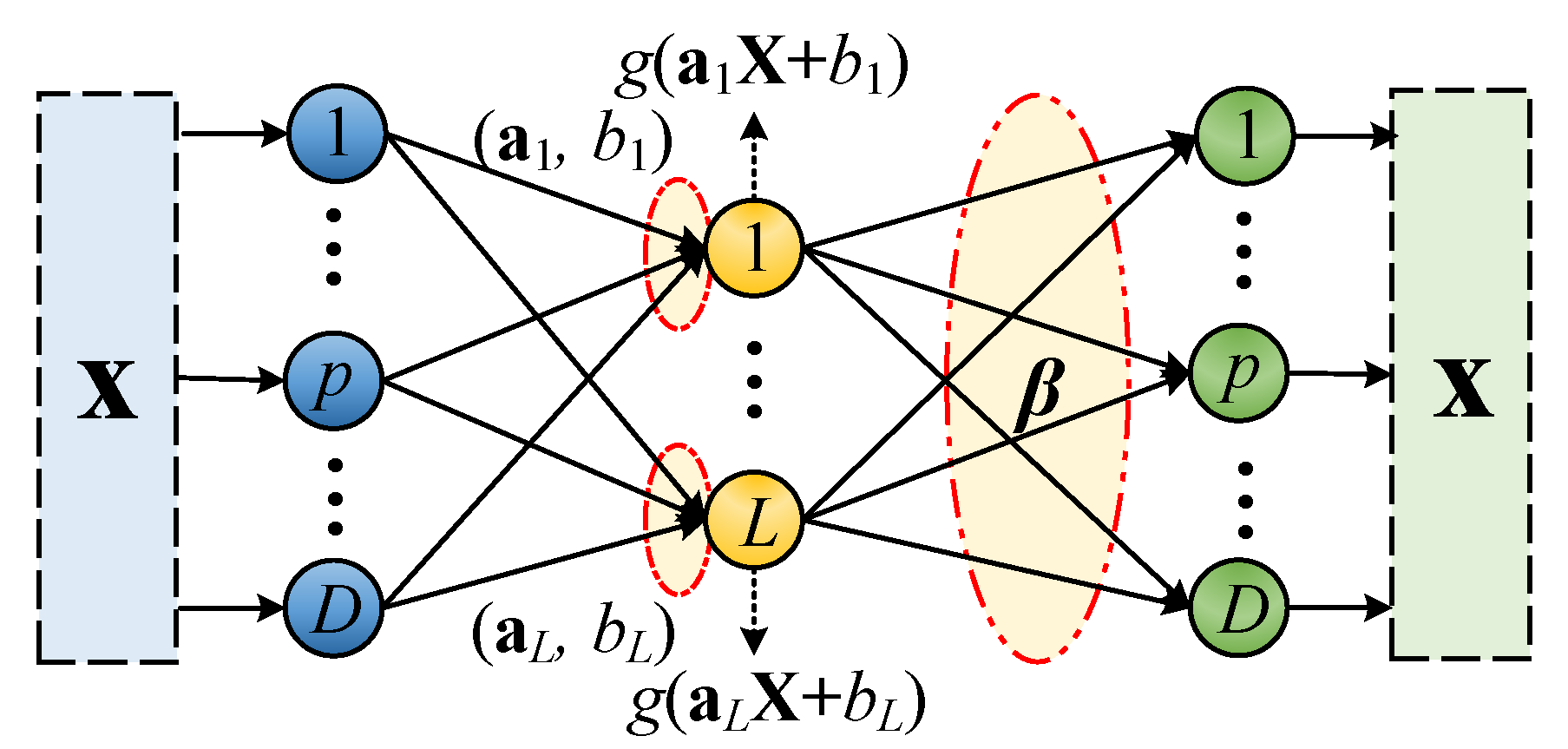
In ELM-AE, the output data were the same as the input data shown Figure 3. The output weight β represents the information transformation from the feature space to input data. The steps of initializing input weights of ELM through ELM-AE are described in Algorithm 2.
Algorithm 2 Input Weight Initialization of LUBE
Input:
Training dataset { X } = { x i | x i ,   i = 1 , 2 , , n } ;
The number of hidden layer nodes of ELM-AE L.
Output:
Input weight matrix of LUBE
(a) Randomly generate the input weight matrix a and bias vector b of the ELM-AE hidden nodes.
(b) Orthogonalize a and b:
a T a = I ,   b T b = 1
(c) Calculate the output of ELM-AE hidden nodes H
H = [g(al,bl, xi)]i = 1, … n, l = 1, …, L
(d) Calculate output weight β of ELM-AE, and the input matrix of LUBE is βT
β = ( I C + H T H ) 1 H T X

4. Experiment and Results

The bi-hourly solar power data utilized in this paper were collected from a grid-connected photovoltaic (PV) system over two years, from 1 July 2010 to 16 June 2012. The PV system was installed on the rooftop of an academic building located in the Coloane island of Macau. The related two-year data recorded by environmental detector and PV power monitoring in real-time were employed to validate the methods. The data included the date, time, solar radiation, temperature, wind speed, and solar power. In the interval prediction model, the historical time series data of the solar power, Pt−2 and Pt−1, and weather data were generated as input variables to predict Pt. One-step-ahead prediction was carried out in this section. The majority of the data (70%) were regarded as the training dataset, while the rest were the test dataset.

4.1. Parameter Settings

To evaluate the proposed LUBE interval prediction model, several widely used heuristic algorithms, including PSO, DE, SA, and HS, were utilized. The PSO algorithm developed by Kennedy and Eberhart [25] was applied to various fields for its strong convergence performance. The DE algorithm combining the genetic algorithm evolution mechanism with the crossover and mutation operation evolves the population, and DE is suitable to handle non differentiable, such as discrete, problems [26]. SA can accept the worse solution to replace the current optimum by the probabilistic technique, which contributes to high search capacity in a large solution space [27]. HS is a simple meta-heuristic algorithm originated by the improvisation process of jazz musicians, which has been strongly criticized as a special case of the well-established evolution strategies algorithm [28].
The parameter settings of four heuristic algorithms are shown as Table 1. In PSO, the inertia weight linearly decreased from 0.7 to 0.1 in the iteration process. In DE, the crossover constant decreased linearly from 0.3 to 0.1 as the iteration increased. In HS, the pitch adjusting rate and bandwidth descended linearly within the range of (0.05, 1) and (1, 50). These algorithms with different characteristics would require different maximum iteration time for an anticipant result. The PSO, which is good at local optimum could converge within a fewer number of iterations. However, SA and HS, as global optimum algorithms, require more iterations to optimize intensively. Thus, the maximum iteration times of the PSO, SA, HS, and DE algorithms re set to 500, 10,000, 2500, and 500, respectively.
In ELM, the number of hidden layer neurons and the tradeoff parameter C were set to 188 and 512 through the point prediction and 5-fold cross-validation technique.
Considering the slight difference of the training and test data, the δ of CWC used equal to 93% in the training set and 90% in the test set, separately. The η was selected as 50 to greatly penalize prediction intervals with a coverage probability lower than δ. In order to leave a certain margin of optimization and avoid being trapped in local optimum, the expected PICP, φ, was set at 95%.
The experiments with different initialization approaches and heuristic algorithms were conducted. Each case was repeated five times to reduce the randomness influence of the dataset partitioning and heuristic algorithms. All experiments in this paper were implemented on a personal notebook computer with i5-4210U CPU and the 8 GB memory.

4.2. Computational Results

In the experiments, the width initialization, point initialization, and random initialization approaches were abbreviated as WI, PI and RI. The terms w/ ELM-AE and w/o ELM-AE mean the initialization approach with ELM-AE and without ELM-AE, respectively.
Table 2, Table 3, Table 4 and Table 5 summarize the average and worst values of the different cases w/ and w/o ELM-AE. Due to the randomness character of the heuristic algorithm, it obtained different results for each optimization, so the result of the average and worst cases can have a comprehensive understanding of the performance and robustness of the algorithms. In Table 2 and Table 3, the average case of HS for PI obtained a CWC of 49.36%, but the worst result was 66.4%. In Table 4 and Table 5, the average case of SA for WI acquired a CWC of 67.86%, but the worst result was 145.29%, which was almost twice as much as the average case. The model combining PSO with WI w/ ELM-AE produced the best and the most stable prediction result among all the cases.
The training accuracy of WI and PI was similar in Table 2, but the WI behaved more stably than PI in the aspect of the test set. In general, The WI was superior to the PI and RI. The RI performed the worst in all the cases.
Comparing Table 2 with Table 3, the initialization approach with ELM-AE was better than the one without ELM-AE. The ELM-AE can significantly improve the prediction performance of RI in both of the training and test datasets. In PI and WI, the CWC of the training set with ELM-AE was higher than the one without ELM-AE. However, the performance of the test set was the reverse. It is implied that the ELM-AE can reduce the over-fitting phenomenon in the training process, and improve the stability of the test set by impairing the random impact of initial weight.

4.2.1. Result Analysis 1—Initialization Approach

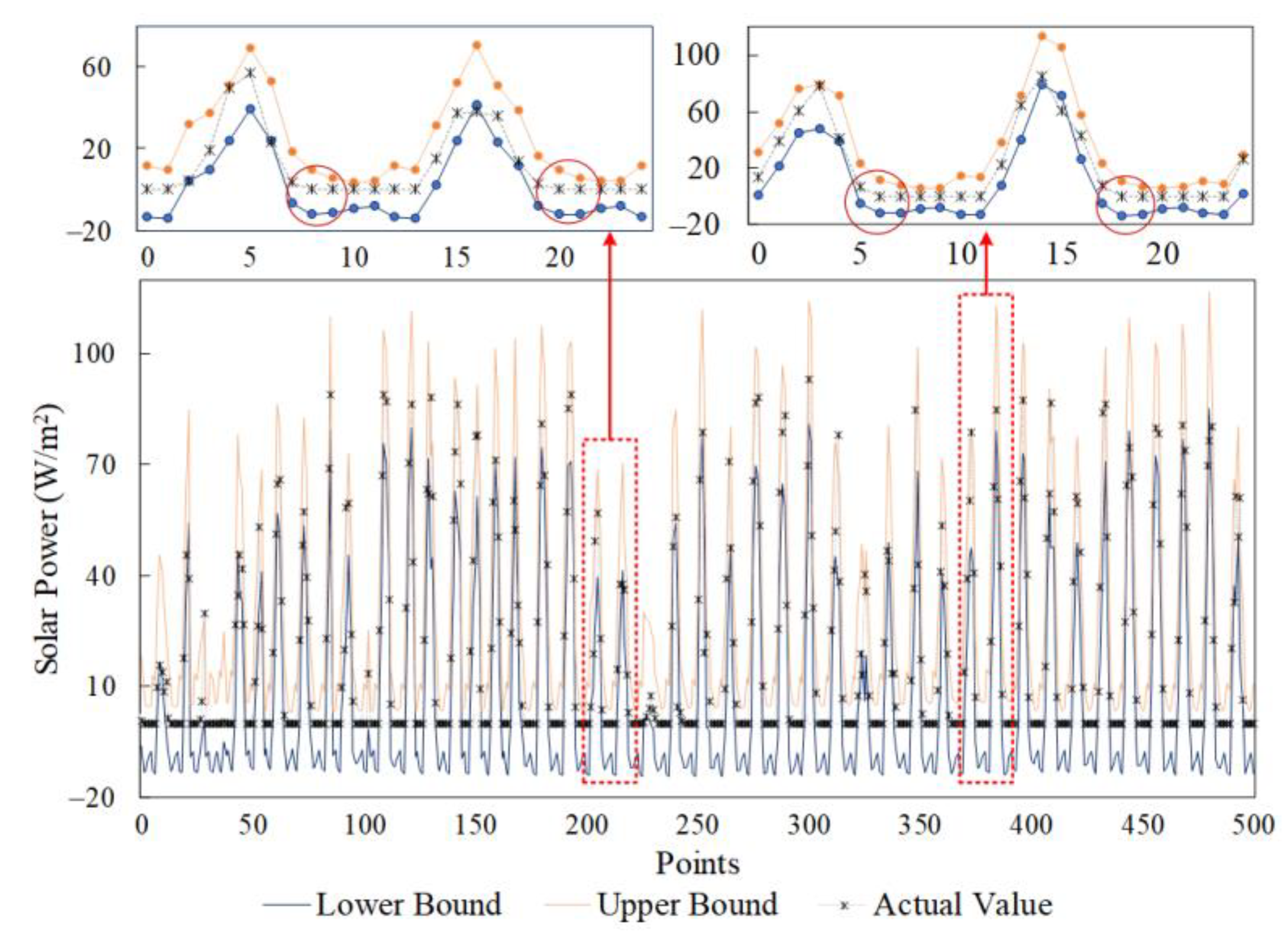
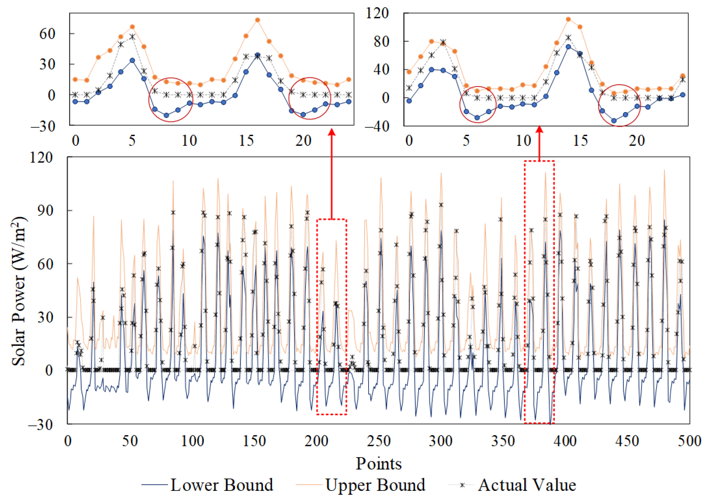
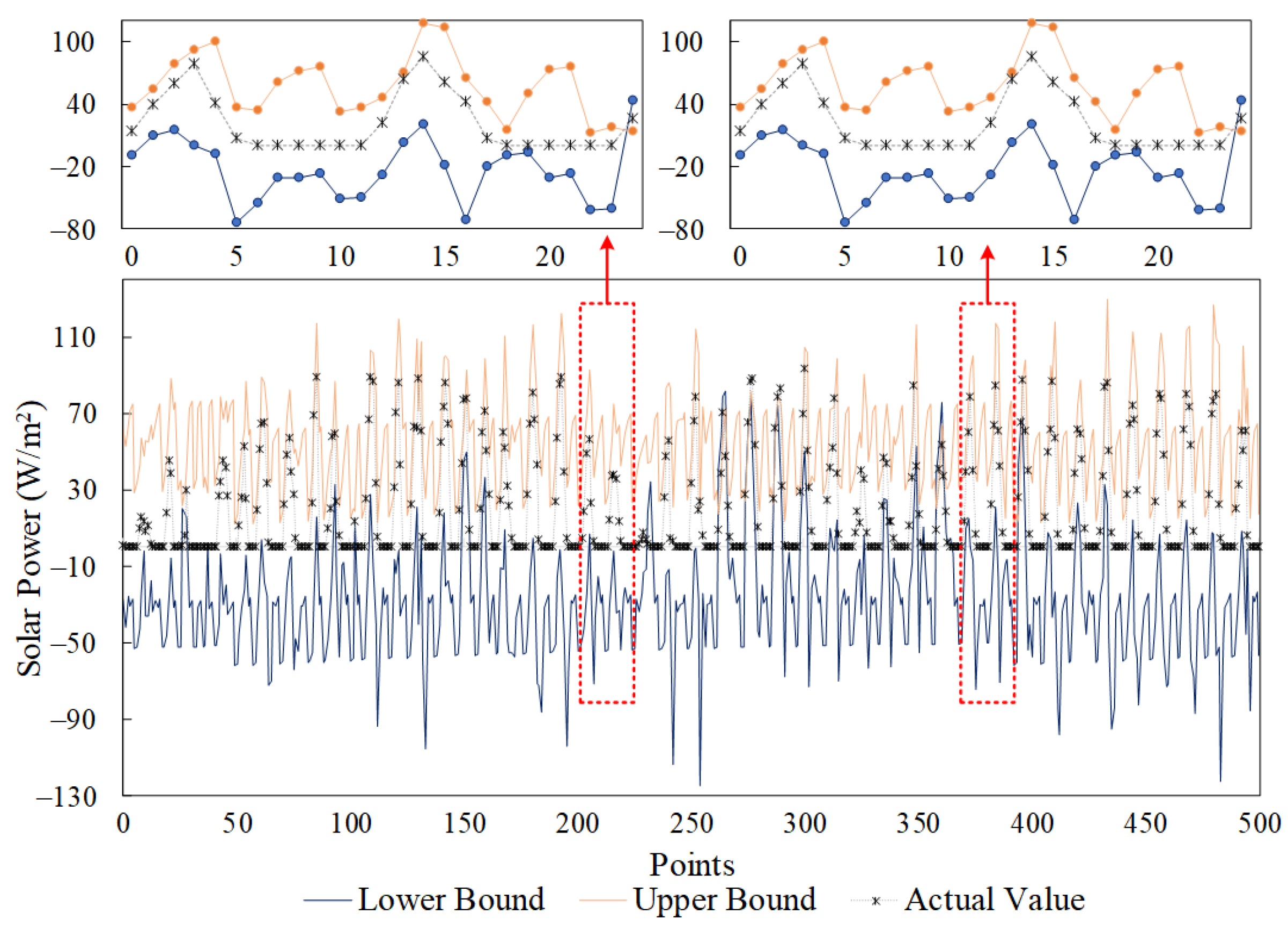
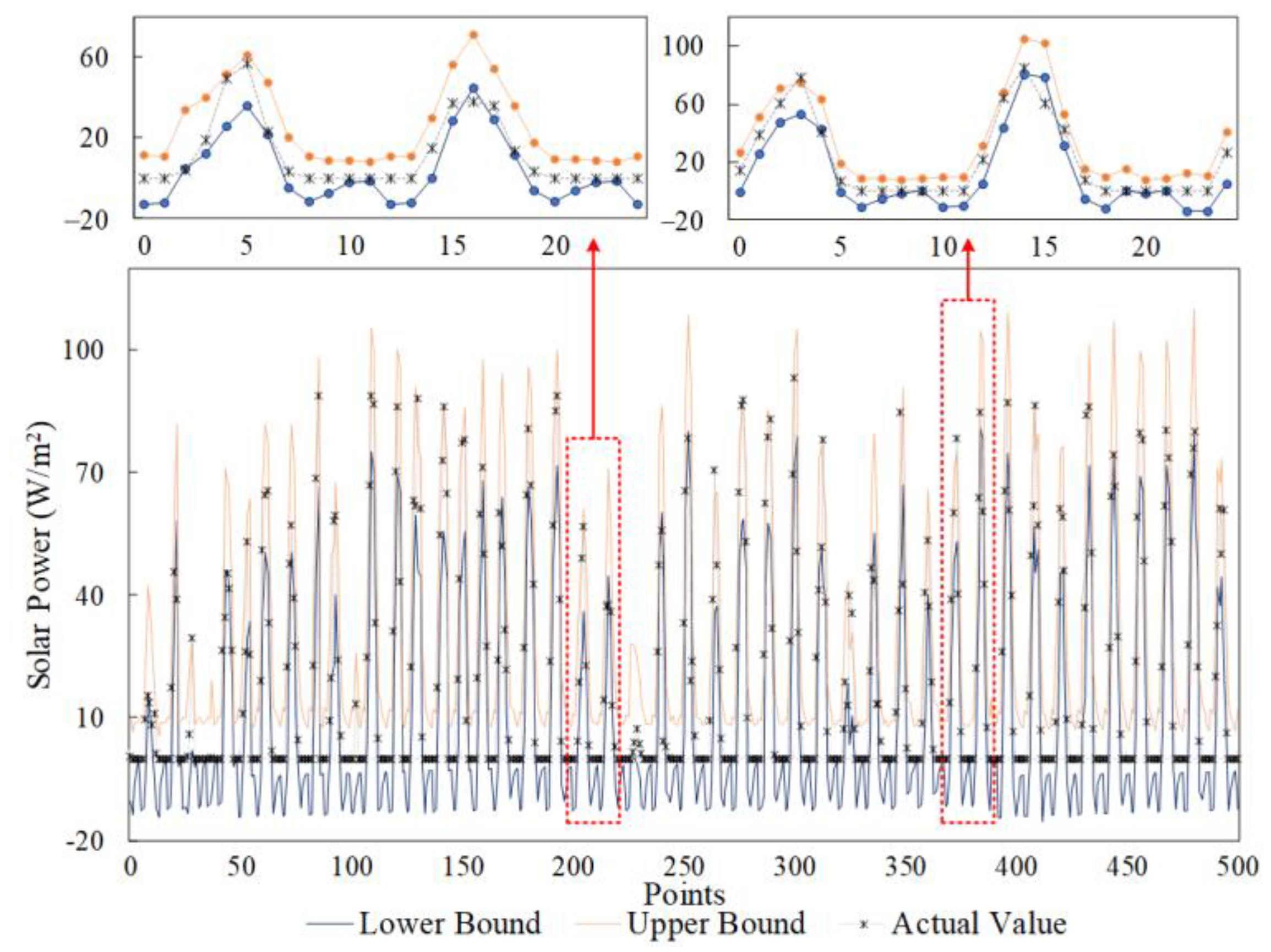
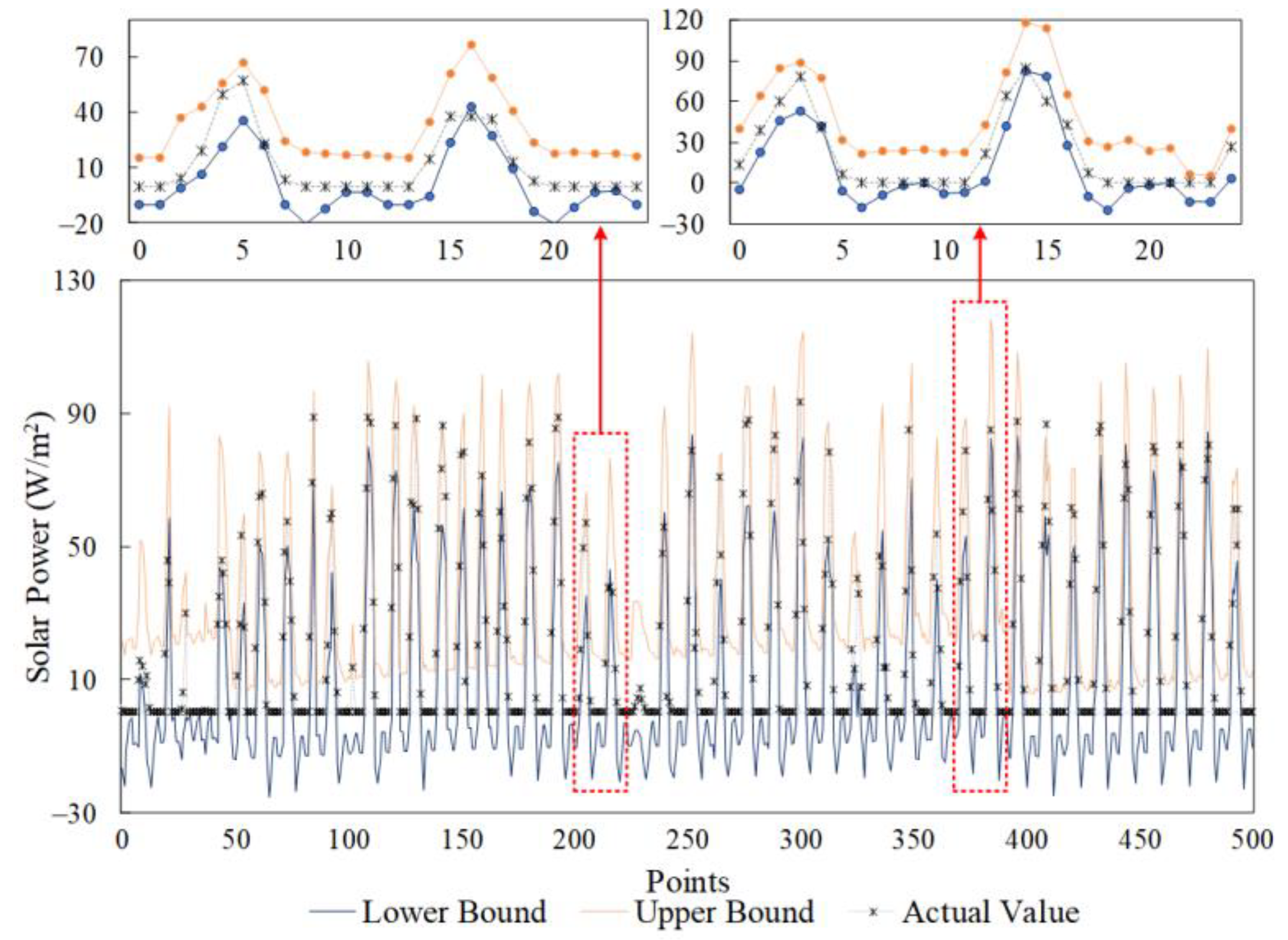
The prediction interval results employing different initialization approaches with ELM-AE and PSO are shown in Figure 4, Figure 5 and Figure 6. It is clear that most actual power points can be covered in the interval due to the expected PICP equal to 0.93.
In the enlarged views of Figure 4 and Figure 5, both of the predicted boundaries of WI and PI can accurately trace the fluctuation of the power curve and preform similarly.
However, in the turning points, such as the 8th and 20th points in the left view and the 6th and 18th points in the right view, the predicted interval of WI was narrower than PI. Thus, the whole predicted interval of WI was more uniform than PI and its predicted result was better, which is in accordance with Table 2.
In Table 2, Table 3, Table 4 and Table 5, for the average test result, the best PINRW for RI was 114.58%, while the worst result for PI and WI was 49.36%. The PINRW of RI was much larger than WI and PI. Thus, the predicted interval of RI intends to employ a universal upper and lower limit to cover as many points as possible, as shown in Figure 6, which has no guidance function.
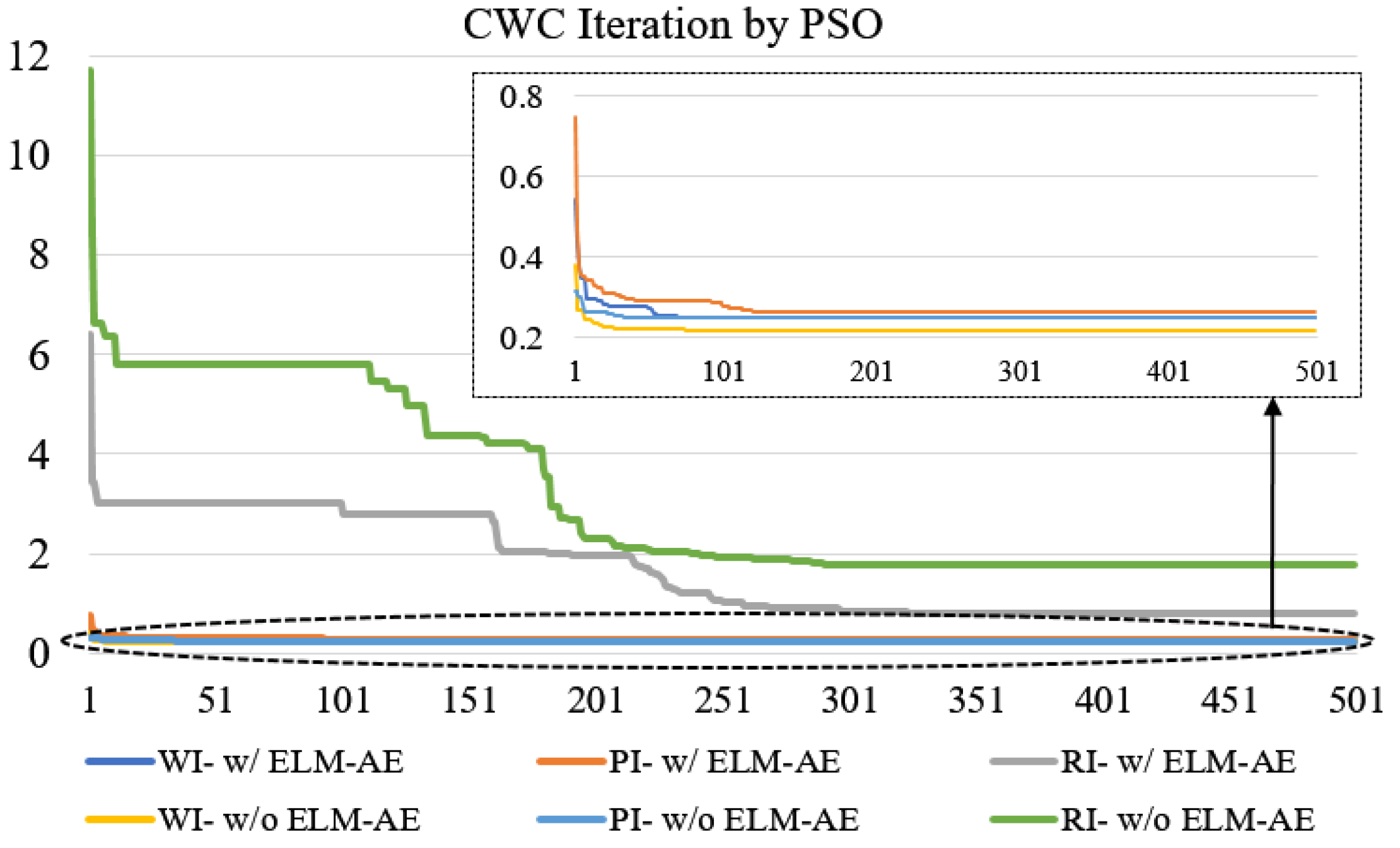
The CWC convergence curves of PSO for different cases are shown as representative in Figure 7. It is apparent that the CWC initial values in RI were significantly larger than other non-random initialization ways. The curves of RI almost converged around 250 iterations. The WI and PI could achieve stable values around 100 iterations. Besides, the converged value of RI was much larger than the WI and PI. Thus, it is concluded that the RI is not a good choice of LUBE initialization.

4.2.2. Result Analysis 2—ELM-AE

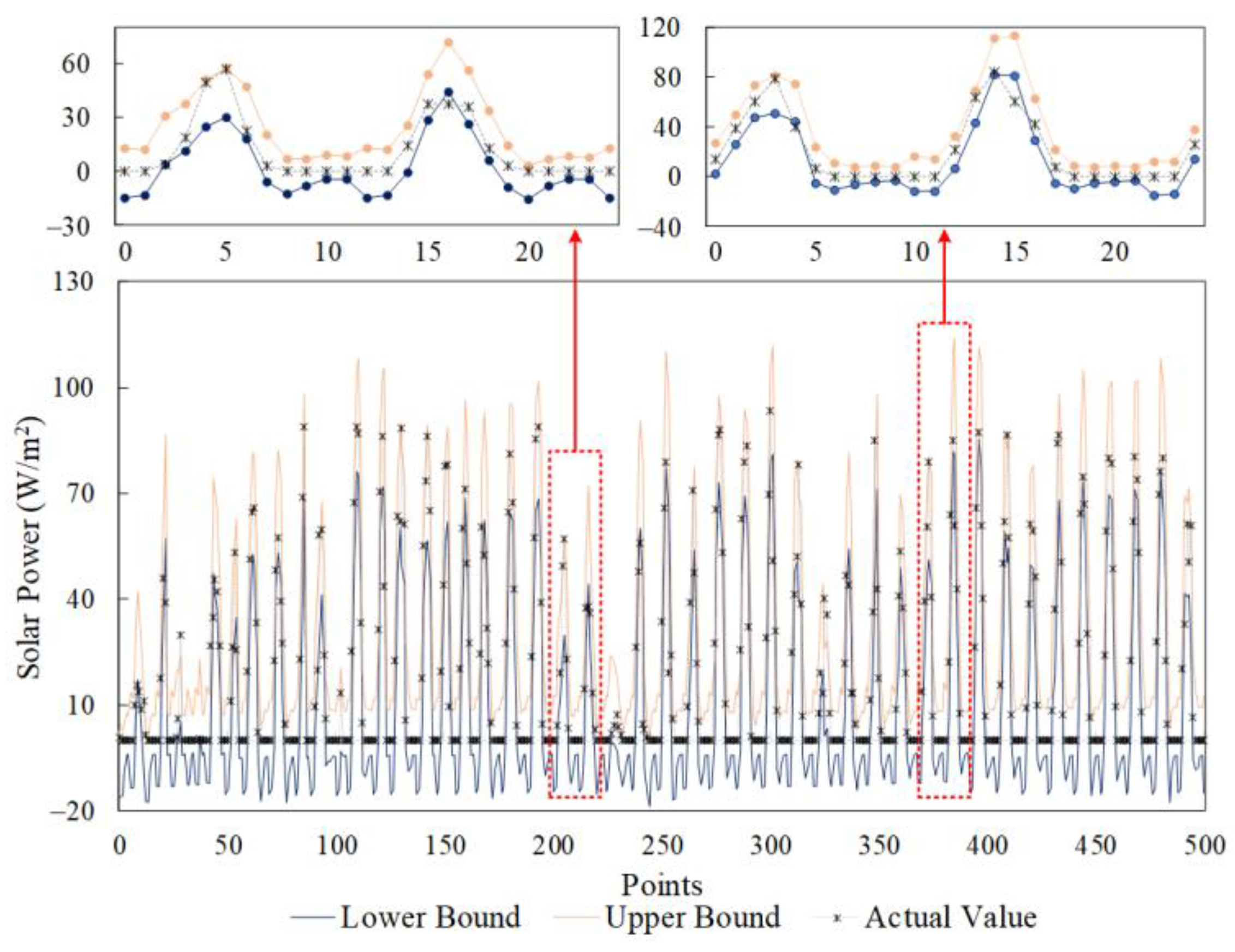
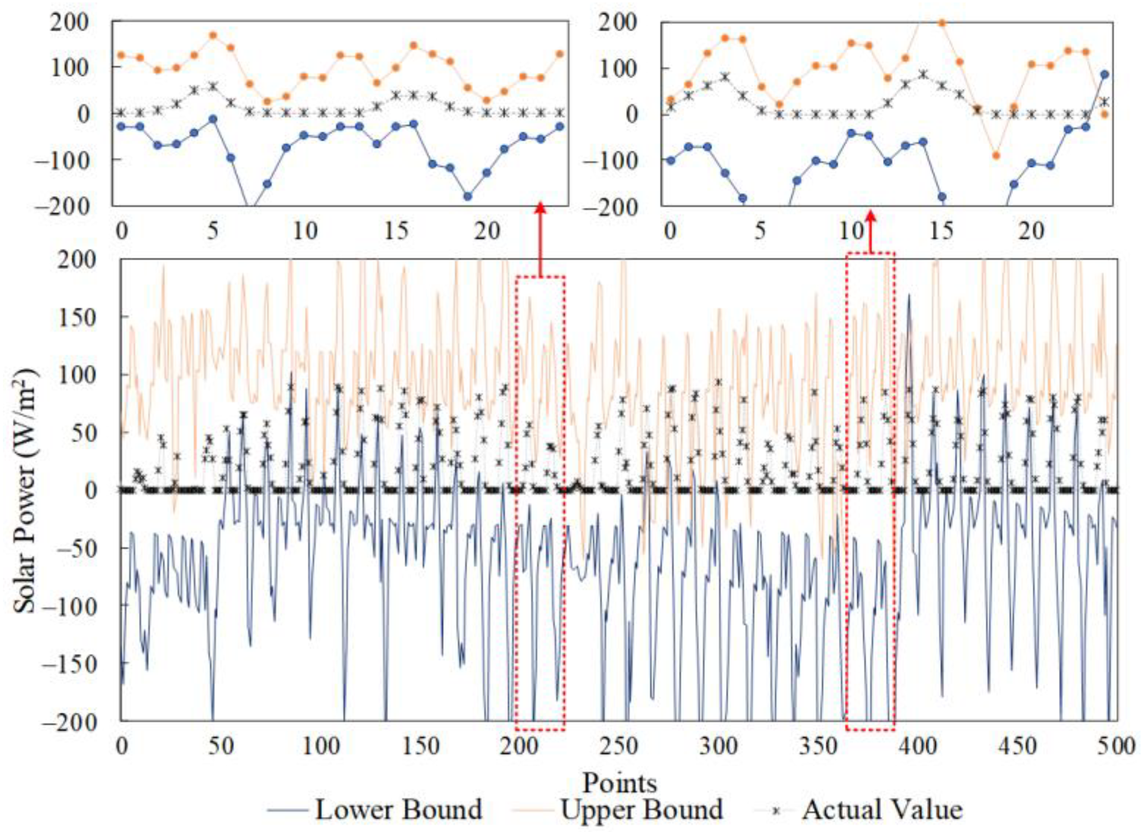
Figure 8, Figure 9 and Figure 10 display the predicted intervals by WI, PI, and RI w/o ELM-AE. Comparing Figure 4 and Figure 5 with Figure 8 and Figure 9, it is apparent that no matter whether or not the WI and PI utilized ELM-AE, their performances were generally close. In the enlarged views, the predicted interval of WI and PI w/o ELM-AE was narrower than the one with ELM-AE, especially points in the night. This is because the ELM-AE impaired the randomness impact of LUBE, which also reduced the diversity of the solutions and further impacted the optimal solution evolution. Thus, the initialization approach w/o ELM-AE had a higher chance of obtaining the global optimal solution than the one w/ ELM-AE, but it also caused unstable performances due to the over-fitting phenomenon.
When ELM-AE was not utilized in RI in Figure 10, the performance dropped drastically, resulting in the fluctuation range of interval reaching ±200. Thus, the employment of ELM-AE can facilitate RI by reducing the divergence of the model.
To clearly explain the role of ELM-AE, the characteristics of the input weight matrix of ELM in LUBE was analyzed in detail. The rank of the input weight matrix was not influenced. The mean absolute value of the input weight matrix grew down from 0.5014 to 0.1146 and the matrix sparsity dropped from 0.2451 to 0.1368 after adding ELM-AE. Thus, the ELM-AE displays the role of the feature extraction and weakens the overfitting of the trained model.

4.2.3. Result Analysis 3—Heuristic Algorithm

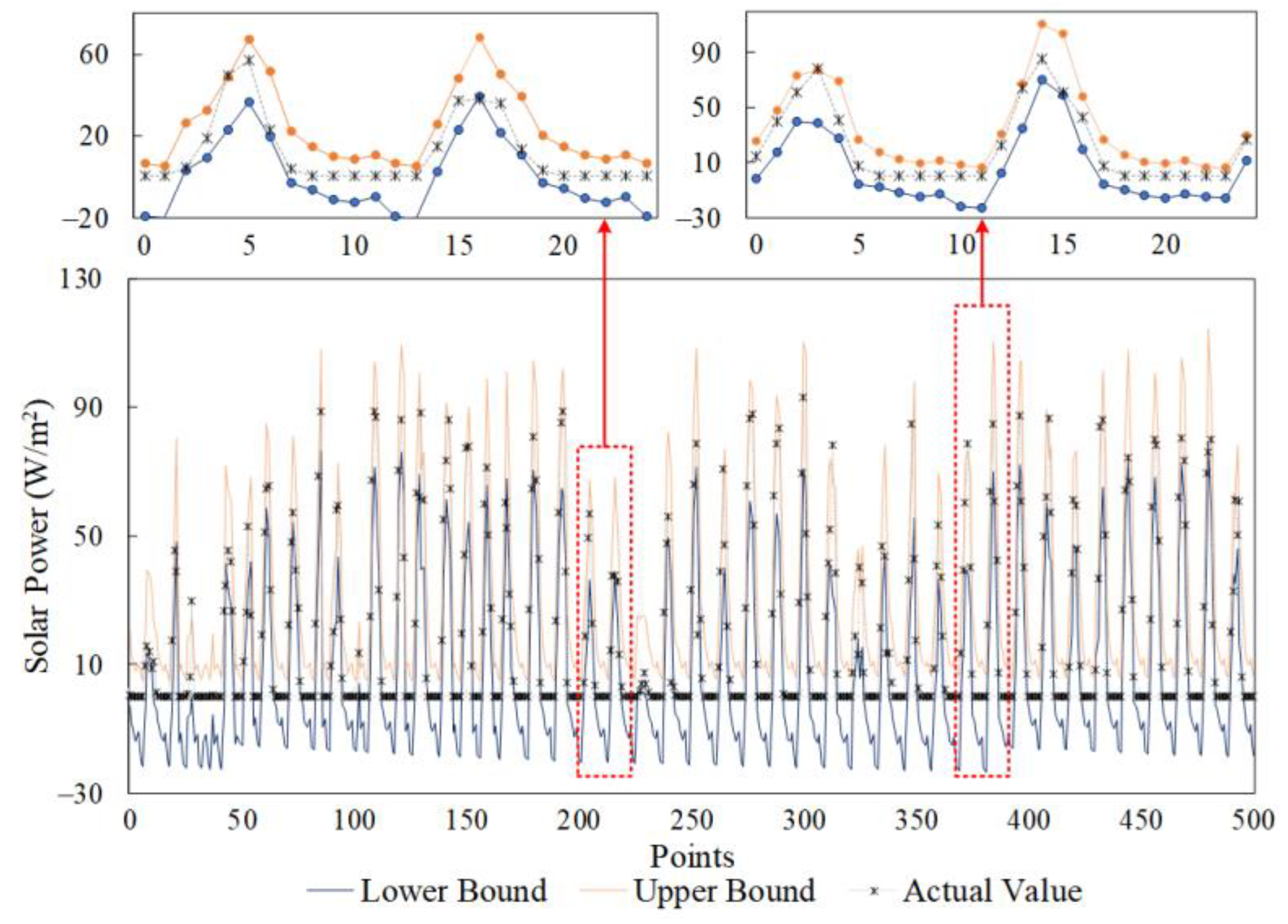
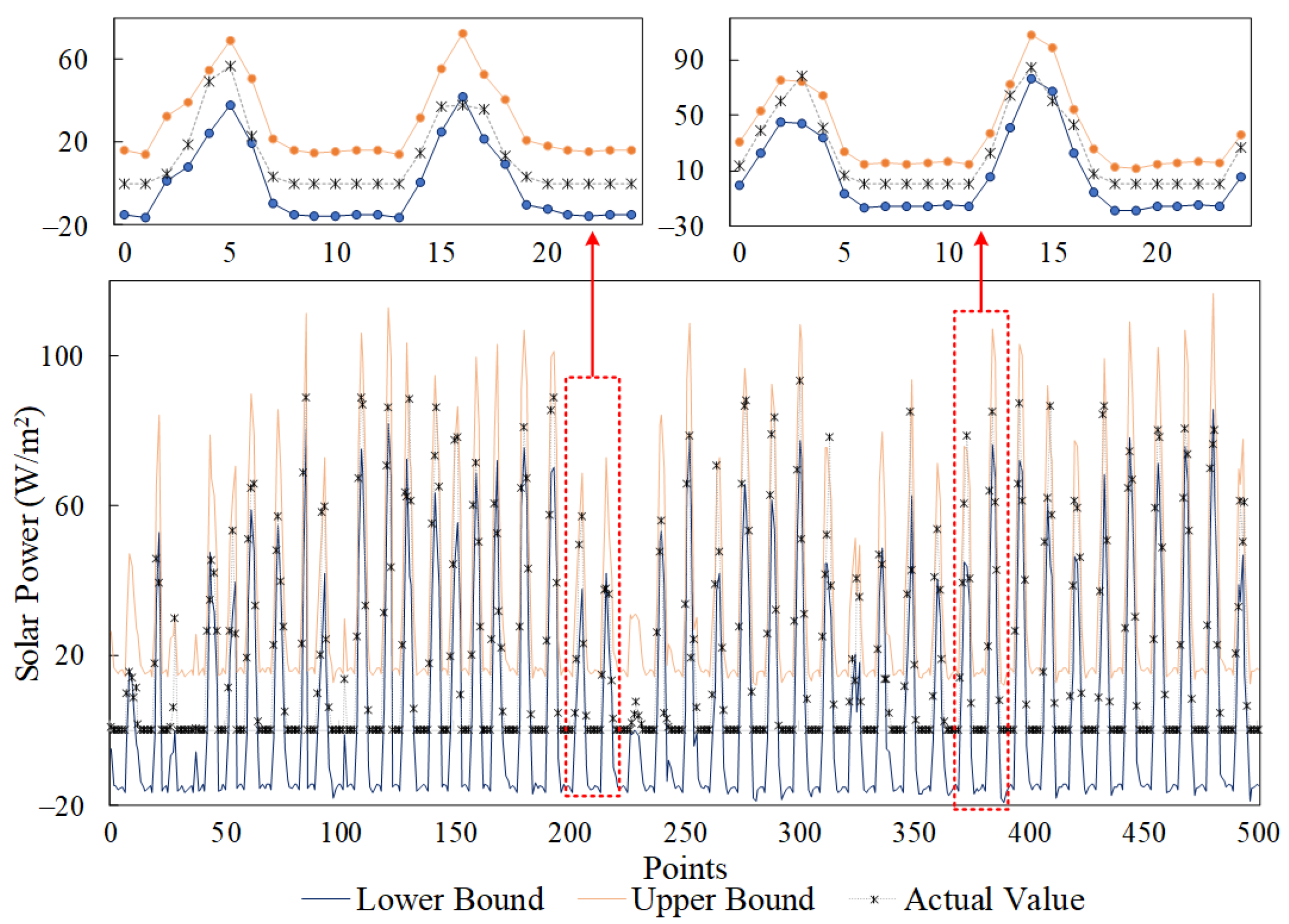
To display performances of different heuristic algorithms, the prediction intervals through the WI w/ ELM-AE model optimized by SA and HS are shown in Figure 11 and Figure 12. It is obvious that the lower bounds in Figure 11 and Figure 12 are lower than the one in Figure 4, resulting in the wider prediction interval. The PSO preformed the best among all the heuristic algorithms. In theory, the SA, HS, and DE algorithms have better global optimum search capacity than PSO. However, in the case of LUBE prediction interval, their evolutionary efficiencies were too low and could not obtain a good result in the limited computational time. In Table 2 and Table 4, the prediction results of the HS and DE are the same for WI. This is because their optimal solutions, obtained in the initialization, stayed the same in the whole progress due to their low evolutionary efficiency.
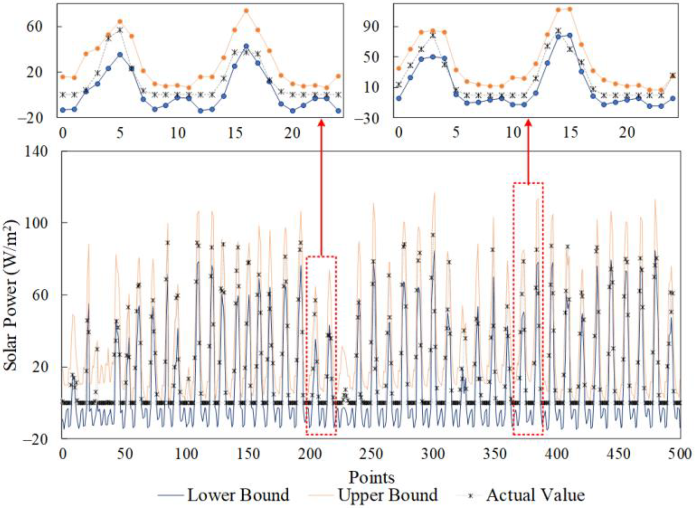
Figure 13 and Figure 14 display the predicted interval optimized by SA and HS based on WI w/o ELM-AE. Combined with Table 3 and Table 5, the trained LUBE prediction model displayed obvious over-fitting phenomenon. The PSO ha the most serious over-fitting phenomenon among all the heuristic algorithms due to its good capacity of solving optimization problems.
The iterative time for various heuristic algorithms is another factor affecting the model performance, especially for online prediction. Average computational times for different heuristic algorithms and initialization approaches are shown in Table 6 and Table 7. The training time is directly impacted by the evaluation times of the cost function. The evaluation times of PSO, SA, HS, and DE were 50,000, 50,000, 62,500, and 50,000, respectively. The running time of PSO and DE was close and the SA cost the most computational time. Comparing Table 6 with Table 7, it is obvious that the experiments without ELM-AE ran longer than the ones with ELM-AE in all cases. This is because the ELM-AE makes the input weight matrix of the LUBE sparse, which reduces the computational load and cuts down the time.

5. Conclusions

Renewable energy generation forecasting technology contributes to decreasing the uncertainty and randomness of renewable resources and can provide essential reference information for the scheduling and operation of the power system. Interval prediction with a statistical confidence level is good at quantifying the uncertainties of the forecasting power. This paper proposed a new LUBE interval prediction framework based on the point prediction technology of ELM. The ELM-AE was employed to generate input weight matrix βT; then PI width initialization way acquired the initial output weight matrix w0, satisfying the presupposed PICP. Finally, the output weights of ELM were further optimized through a heuristic algorithm. Four algorithms, PSO, DE, SA, and HS, were implemented to verify the performance of the proposed mechanism. Different experimental settings were combined into different contrast experiments to validate and analyze the impacts of different settings on the model performance.
The prediction performance of WI was slightly superior to the property of PI generally. At some power curve turning points, WI could more reasonably constrain the prediction interval and avoid a large prediction margin. The simulation experiments revealed that ELM-AE could significantly decrease the matrix sparsity and the mean absolute value of the input weight matrix, which are statistically equal to 0.5 when the matrix is randomly generated from a uniform random distribution between (−1, 1). The over-fitting of the learned model was weakened and the generalization ability of the model improved when using ELM-AE. The PSO algorithm achieved the best prediction performance among the four algorithms under various situations. The SA, HS, and DE algorithms performed poorly in the limited computational time, and the HS and DE algorithms could hardly further optimize the output weight matrix. The performance of the model was also constrained by the limitations of the heuristic algorithms and was related to the algorithm parameters. However, the PSO resulted in the most severe over-fitting phenomenon for a sharp prediction interval. In general, the proposed LUBE model with a new model initialization approach would acquire a faithful prediction interval with more detailed optimization and stable generalization performance.
Although the LUBE approach can forecast the interval covering the solar power accurately, the width of prediction intervals at different times of day was consistent. However, it is apparent that the power value is zero in the night and that the nighttime interval can be narrower. The mechanism of LUBE makes the width of interval in different periods consistent, which deserves improvement in further research. Some normal optimization technique for neural networks also can be added to the prediction model framework to improve the learning performance, such as the ensemble learning of multiple neural networks. The evaluation fitness function transforms the original multi-objective problem into a single-objective problem for simplification. CWC could effectively guarantee the PICP of prediction intervals, but the penalty term also restricts and intervenes in the search for an optimal solution, which results in some feasible solutions being unavailable. In the future, it is expected to explore a new evaluation mechanism that could systematically balance the coverage probability and the width of the prediction interval.

Acronyms

CWCCoverage width-based criterion
DEDifferential evolution
ELM-AEELM auto encoder
HSHarmony search
LRIElinear regression interval estimation
LUBELower and upper bound estimation
NNNeural network
PIPoint initialization approach
PVPhotovoltaic
PICPPrediction interval coverage probability
PINRWPI normalized root-mean-square width
PSOParticle swarm optimization
RIRandom initialization approach
SASimulated annealing
WIWidth initialization approach
w/ ELM-AEInitialization approach with ELM-AE
w/o ELM-AEInitialization approach without ELM-AE
ELMExtreme learning Machine

Author Contributions

H.L. supervised the project and designed the experiment. Resources and data curation, P.L.; writing—original draft preparation, C.Z.; writing—review and editing, H.L.

Funding

This research was funded by the Science and Technology Program of State Grid Corporation of Zhejiang Province under Grand 5211DS17001Z, the National Natural Science Foundation of China under Grant 51807023, Natural Science Foundation of Jiangsu Province under Grant BK20180382.

Conflicts of Interest

The authors declare no conflict of interest.

References

  1. Khosravi, A.; Mazloumi, E.; Nahavandi, S.; Creighton, D.; Lint, J.W.C.V. Prediction intervals to account for uncertainties in travel time prediction. IEEE Trans. Intell. Transp. Syst. 2011, 12, 537–547. [Google Scholar] [CrossRef]
  2. Saez, D.; Avila, F.; Olivares, D.; Canizares, C.; Marin, L. Fuzzy prediction interval models for forecasting renewable resources and loads in microgrids. IEEE Trans. Smart Grid 2015, 6, 548–556. [Google Scholar] [CrossRef]
  3. He, Y.; Liu, R.; Li, H.; Wang, S.; Lu, X. Short-term power load probability density forecasting method using kernel-based support vector quantile regression and copula theory. Appl. Energy 2017, 185 Pt 1, 254–266. [Google Scholar] [CrossRef]
  4. Tahmasebifar, R.; Sheikh-El-Eslami, M.K.; Kheirollahi, R. Point and interval forecasting of real-time and day-ahead electricity prices by a novel hybrid approach. IET Gener. Transm. Distrib. 2017, 11, 2173–2183. [Google Scholar] [CrossRef]
  5. Yang, X.; Ma, X.; Kang, N.; Maihemuti, M. Probability interval prediction of wind power based on kde method with rough sets and weighted markov chain. IEEE Access 2018, 6, 51556–51565. [Google Scholar] [CrossRef]
  6. Yun, S.L.; Scholtes, S. Empirical prediction intervals revisited. Int. J. Forecast. 2014, 30, 217–234. [Google Scholar]
  7. Sheng, C.; Zhao, J.; Wang, W.; Leung, H. Prediction intervals for a noisy nonlinear time series based on a bootstrapping reservoir computing network ensemble. IEEE Trans. Neural Netw. Learn. Syst. 2013, 24, 1036–1048. [Google Scholar] [CrossRef]
  8. MacKay, D.J.C. The evidence framework applied to classification networks. Neural Comput. 1992, 4, 720–736. [Google Scholar] [CrossRef]
  9. Veaux, R.D.D.; Schumi, J.; Ungar, S.L.H. Prediction intervals for neural networks via nonlinear regression. Technometrics 1998, 40, 273–282. [Google Scholar] [CrossRef]
  10. Kothari, S.C.; Oh, H. Neural Networks for Pattern Recognition. Adv Comput. 1993. Available online: https://books.google.com.hk/books?id=vL-bB7GALAwC&pg=PA165&lpg=PA165&dq=Kothari,+S.C.;+Oh,H.+Neural+Networks+for+Pattern+Recognition.&source=bl&ots=9dkbD_qwsK&sig=ACfU3U16HyCBDuZ2wEYkBNXD5MnuaqQ58Q&hl=zh-TW&sa=X&ved=2ahUKEwiY5rXG0MPlAhXLc94KHWtkAnMQ6AEwAHoECAoQAQ#v=onepage&q=Kothari%2C%20S.C.%3B%20Oh%2CH.%20Neural%20Networks%20for%20Pattern%20Recognition.&f=false (accessed on 30 October 2019).
  11. Trapero, J.R. Calculation of solar irradiation prediction intervals combining volatility and kernel density estimates. Energy 2016, 114, 266–274. [Google Scholar] [CrossRef] [Green Version]
  12. Taylor, J.W.; Mcsharry, P.E.; Buizza, R. Wind power density forecasting using ensemble predictions and time series models. IEEE Trans. Energy Convers. 2009, 24, 775–782. [Google Scholar] [CrossRef]
  13. Khosravi, A.; Nahavandi, S.; Creighton, D.; Atiya, A.F. Lower upper bound estimation method for construction of neural network-based prediction intervals. IEEE Trans. Neural Netw. 2011, 22, 337–346. [Google Scholar] [CrossRef] [PubMed]
  14. Quan, H.; Srinivasan, D.; Khosravi, A. Short-term load and wind power forecasting using neural network-based prediction intervals. IEEE Trans. Neural Netw. Learn. Syst. 2017, 25, 303–315. [Google Scholar] [CrossRef] [PubMed]
  15. Wan, C.; Niu, M.; Song, Y.; Xu, Z. Pareto optimal prediction intervals of electricity price. IEEE Trans. Power Syst. 2017, 32, 817–819. [Google Scholar] [CrossRef]
  16. Shi, Z.; Liang, H.; Dinavahi, V. Wavelet neural network based multiobjective interval prediction for short-term wind speed. IEEE Access 2018, 6, 63352–63365. [Google Scholar] [CrossRef]
  17. Yadav, A.K.; Chandel, S.S. Solar radiation prediction using artificial neural network techniques: A review. Renew. Sustain. Energy Rev. 2014, 33, 772–781. [Google Scholar] [CrossRef]
  18. Li, Z.; Liu, X.; Chen, L. Load interval forecasting methods based on an ensemble of Extreme Learning Machines. In Proceedings of the IEEE Power and Energy Society General Meeting, Denver, CO, USA, 26–30 July 2015. [Google Scholar]
  19. Kavousi-Fard, A.; Khosravi, A.; Nahavandi, S. A new fuzzy-based combined prediction interval for wind power forecasting. IEEE Trans. Power Syst. 2015, 31, 18–26. [Google Scholar] [CrossRef]
  20. Jiang, P.; Li, R.; Li, H. Multi-objective algorithm for the design of prediction intervals for wind power forecasting model. Appl. Math. Model. 2019, 67, 101–122. [Google Scholar] [CrossRef]
  21. Ak, R.; Li, Y.F.; Vitelli, V.; Zio, E.; Jacintod, C.M.C. NSGA-II-trained neural network approach to the estimation of prediction intervals of scale deposition rate in oil & gas equipment. Expert Syst. Appl. 2013, 40, 1205–1212. [Google Scholar] [Green Version]
  22. Huang, G.B.; Zhu, Q.Y.; Siew, C.K. Extreme learning machine: Theory and applications. Neurocomputing 2006, 70, 489–501. [Google Scholar] [CrossRef]
  23. Kasun, L.L.C.; Zhou, H.; Huang, G.; Vong, C. Representational Learning with Extreme Learning Machine for Big Data. IEEE Intell. Syst. 2013, 28, 31–34. [Google Scholar]
  24. Xiong, L.; Jiankun, S.; Long, W.; Weiping, W.; Wenbing, Z.; Jinsong, W. Short-term wind speed forecasting via stacked extreme learning machine with generalized correntropy. IEEE Trans. Ind. Inform. 2018, 14, 4963–4971. [Google Scholar]
  25. Eberhart, R.; Kennedy, J. Particle swarm optimization. In Proceedings of the IEEE International Conference on Neural Networks, Perth, Australia, 27 November–1 December 1995; Volume 4, pp. 1942–1948. [Google Scholar]
  26. Storn, R.; Price, K. Differential evolution—A simple and efficient heuristic for global optimization over continuous spaces. J. Glob. Optim. 1997, 11, 341–359. [Google Scholar] [CrossRef]
  27. Kirkpatrick, S.; Gelatt, C.D.; Vecchi, M.P. Optimization by simulated annealing. Science 1983, 220, 671–680. [Google Scholar] [CrossRef] [PubMed]
  28. Geem, Z.W.; Kim, J.H.; Loganathan, G.V. A New Heuristic Optimization Algorithm: Harmony Search. Simulation 2001, 76, 60–68. [Google Scholar] [CrossRef]
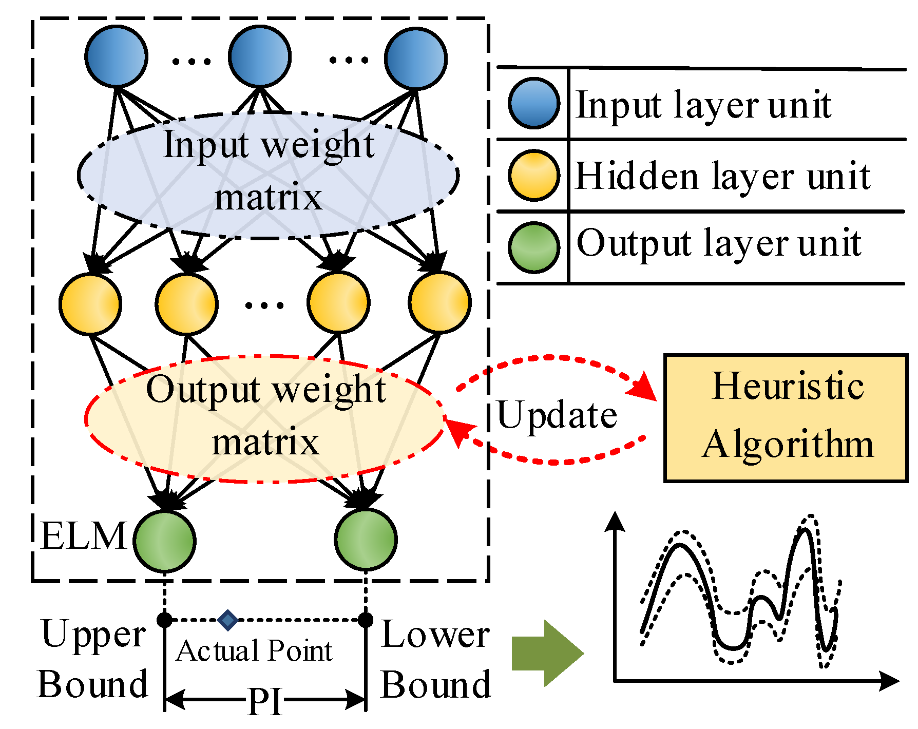
Figure 1. The schematic diagram of the lower and upper bound estimation (LUBE).
Energies 12 04146 g001
Figure 2. The model initialization approach.
Energies 12 04146 g002
Figure 3. The structure of ELM-AE.
Energies 12 04146 g003
Figure 4. The prediction results obtained by PSO and WI with ELM-AE.
Energies 12 04146 g004
Figure 5. The prediction results obtained by PSO and PI with ELM-AE.
Energies 12 04146 g005
Figure 6. The prediction result obtained by PSO and RI with ELM-AE.
Energies 12 04146 g006
Figure 7. CWC of the best solution in training process for PSO.
Energies 12 04146 g007
Figure 8. The prediction results obtained by PSO and WI w/o ELM-AE.
Energies 12 04146 g008
Figure 9. The prediction result obtained by PSO and PI w/o ELM-AE.
Energies 12 04146 g009
Figure 10. The prediction result obtained by PSO and RI w/o ELM-AE.
Energies 12 04146 g010
Figure 11. The prediction results obtained by SA and WI w/ ELM-AE.
Energies 12 04146 g011
Figure 12. The prediction result obtained by HS with WI w/ ELM-AE.
Energies 12 04146 g012
Figure 13. The prediction result obtained by SA and WI w/o ELM-AE.
Energies 12 04146 g013
Figure 14. The prediction result obtained by HS and WI w/o ELM-AE.
Energies 12 04146 g014
Table 1. Parameter settings of heuristic algorithms.
AlgorithmsParameterValue
PSOParticle size100
Inertia weight(0.1, 0.7)
Cognitive acceleration constant1.5
Social acceleration constant2.5
DEPopulation size100
Scaling factor F0.005
Crossover parameter CR(0.1, 0.3)
SAInitial temperature5
Re-annealing interval50
Cooling factor0.9
HSHarmony memory size25
Harmony memory considering rate0.98
Pitch adjusting rate(0.05, 0.1)
Bandwidth(1, 50)
Table 2. Comparison of average results of different cases with ELM-AE.
AVERAGEWI w/ELM-AEPI w/ELM-AERI w/ELM-AE
CWCPICPPINRWCWCPICPPINRWCWCPICPPINRW
PSOTraining26.64%93.01%26.64%26.47%93.01%26.47%117.57%93.01%117.57%
Test25.89%91.30%25.89%35.70%90.90%25.95%114.58%94.14%114.58%
SATraining27.91%93.06%27.91%28.31%93.07%28.31%269.35%93.03%269.35%
Test35.99%91.15%26.78%28.68%91.91%28.68%272.57%93.86%272.57%
HSTraining32.75%94.68%32.75%48.46%95.64%48.46%476.17%96.26%476.17%
Test32.75%93.47%32.75%49.36%94.89%49.36%615.22%95.36%462.11%
DETraining32.75%94.68%32.75%37.22%94.68%37.22%350.1%98.11%350.10%
Test32.75%93.47%32.75%37.47%93.37%37.47%330.66%98.03%330.66%
Table 3. Comparison of the worst results of different cases with ELM-AE.
WORSTWI w/ ELM-AEPI w/ ELM-AERI w/ ELM-AE
CWCPICPPINRWCWCPICPPINRWCWCPICPPINRW
PSOTraining28.19%93.01%28.19%25.94%93.01%25.94%66.04%91.08%66.04%
Test28.28%92.50%28.28%50.35%89.97%24.98%206.21%93.01%206.21%
SATraining28.11%93.03%28.11%28.88%93.16%28.88%328.42%93.03%328.42%
Test27.54%91.88%27.54%29.91%92.32%29.91%337.88%94.32%337.88%
HSTraining34.37%95.04%34.37%66.69%98.27%66.69%371.12%93.41%371.12%
Test34.37%94.05%34.37%66.40%98.76%66.40%908.87%88.55%296.42%
DETraining34.37%95.04%34.37%37.22%94.68%37.22%429.44%99.28%429.44%
Test34.37%94.05%34.37%37.47%93.37%37.47%417.74%98.09%417.74%
Table 4. Comparison of average results of different cases without ELM-AE.
AVERAGEWI w/o ELM-AEPI w/o ELM-AERI w/o ELM-AE
CWCPICPPINRWCWCPICPPINRWCWCPICPPINRW
PSOTraining22.66%93.01%22.36%24.55%93.01%24.55%199.31%93.01%199.31%
Test50.70%89.43%22.56%51.99%89.64%24.17%347.39%91.99%187.52%
SATraining26.36%93.07%26.36%27.07%93.16%27.07%697.12%93.04%697.12%
Test67.86%89.17%25.34%43.98%90.50%27.61%669.95%93.58%669.95%
HSTraining30.48%94.65%30.48%102.92%92.75%33.21%994.26%96.43%994.26%
Test30.56%92.77%30.56%42.28%91.89%34.26%1037.78%97.38%1037.78%
DETraining26.30%93.30%26.30%24.86%93.38%24.86%688.64%96.36%688.64%
Test30.57%90.71%25.77%83.97%89.22%23.72%641.13%94.58%641.13%
Table 5. Comparison of the worst results of different cases without ELM-AE.
WORSTWI w/o ELM-AEPI w/o ELM-AERI w/o ELM-AE
CWCPICPPINRWCWCPICPPINRWCWCPICPPINRW
PSOTraining21.79%93.01%21.79%23.48%93.01%23.48%195.77%93.01%195.77%
Test77.47%88.06%21.30%82.94%87.88%21.36%620.14%87.88%159.74%
SATraining25.25%93.04%25.25%26.08%93.06%26.08%845.49%93.06%845.49%
Test145.29%86.73%23.69%71.09%88.86%25.67%889.78%93.12%889.78%
HSTraining31.25%95.02%31.25%29.88%93.27%29.88%1143.80%97.97%1143.80%
Test31.25%93.16%31.25%69.00%89.35%28.92%1273.26%99.64%1273.26%
DETraining22.45%93.12%22.45%30.29%93.04%30.29%825.84%97.04%825.84%
Test44.69%89.70%20.69%228.93%86.11%28.61%791.94%96.14%791.94%
Table 6. Average computational time (s) for different initialization approaches with ELM-AE.
AlgorithmsWIPIRI
PSO1374.221369.521360.97
SA2235.662224.442223.50
HS1670.621647.881647.88
DE1398.421367.051366.08
Table 7. Average computational time (s) for different initialization approaches without ELM-AE.
AlgorithmsWIPIRI
PSO1533.881673.481484.03
SA2327.962322.452330.64
HS1647.881795.761788.86
DE1474.171469.561465.95