Abstract
The recent developments in combining point forecasts of day-ahead electricity prices across calibration windows have provided an extremely simple, yet a very efficient tool for improving predictive accuracy. Here, we consider two novel extensions of this concept to probabilistic forecasting: one based on Quantile Regression Averaging (QRA) applied to a set of point forecasts obtained for different calibration windows, the other on a technique dubbed Quantile Regression Machine (QRM), which first averages these point predictions, then applies quantile regression to the combined forecast. Once computed, we combine the probabilistic forecasts across calibration windows by averaging probabilities of the corresponding predictive distributions. Our results show that QRM is not only computationally more efficient, but also yields significantly more accurate distributional predictions, as measured by the aggregate pinball score and the test of conditional predictive ability. Moreover, combining probabilistic forecasts brings further significant accuracy gains.
1. Introduction
After 25 years of intensive research, the electricity price forecasting (EPF) literature includes hundreds of publications, focused both on point [1,2] and probabilistic [3,4] predictions. However, very few studies try to find the optimal length of the calibration window or even consider calibration windows of different lengths. Instead, the typical approach has been to select ad-hoc a ‘long enough’ window, ranging from as few as 10 days to as much as five years. Only recently has this issue been tackled more systematically, initially by Hubicka et al. [5] and then in a follow up article by Marcjasz et al. [6]; note, that the latter paper eventually appeared in print earlier than the original study.
Hubicka et al. [5] proposed a novel concept in energy forecasting that combined day-ahead predictions across different calibration windows ranging from 28 to 728 days. Using data from the Global Energy Forecasting Competition 2014, they showed that such averaging across calibration windows yielded better results than selecting ex-ante only one ‘optimal’ window length. They concluded that a mix of a few short- and a few long-term windows led to the best predictions. Marcjasz et al. [6] extended their analysis to other datasets and larger models. More importantly, they introduced a well-performing weighting scheme for averaging forecasts. Overall, their results confirmed earlier findings, but they advised to use slightly longer windows at the shorter end, especially when considering models with more explanatory variables (inputs). On the other hand, they concluded that including 3- instead of 2-year windows did not bring significant benefits. Marcjasz et al. recommended the WAW(56:28:112, 714:7:728) averaging scheme, i.e., past performance weighted combination of forecasts from six windows: 56-, 84-, 112-, 714-, 721- and 728-day long; we use Matlab notation to describe the sets of windows, e.g., (7:364) refers to all windows from 7 to 364 days, (14:7:105) to 14 window lengths: 14, 21, …, 105 days, while (7, 364) to 7- and 364-day windows. In their empirical study, this averaging scheme performed very well and in most cases was not significantly outperformed by any other forecast.
Despite the innovative content, the above mentioned papers are limited to point predictions. To address this gap, here we consider two novel extensions of the averaging across calibration windows concept to probabilistic forecasting: one based on Quantile Regression Averaging (QRA) [7] and one using the Quantile Regression Machine (QRM) [8]. As the underlying statistical technique both use quantile regression [9], which has recently become the workhorse of probabilistic energy forecasting [10,11,12,13,14]. Moreover, both apply it to a pool of point forecasts obtained for calibration windows of different lengths and yield predictions for the 99 percentiles of the next day’s price distribution for each hour. The difference between them lies in the choice of the regressors—QRA uses the point forecasts themselves, while QRM first averages them, then applies quantile regression to the combined forecast. Once computed, we combine the probabilistic forecasts across calibration windows by averaging probabilities of the corresponding predictive distributions, as in [15]. Although the latter works well in our study, the literature on combining predictive distributions offers alternatives [15,16,17,18] which could be considered as well.
Furthermore, since we want to focus on predictive distributions, we do not propose our own approach to point forecasting. Instead we select a well performing model and take its point forecasts as inputs to the QRA and QRM procedures. Our starting point is the study of Marcjasz et al. [6] and the autoregressive expert model they call ARX2, fitted to asinh-transformed day-ahead prices from two major power markets (Nord Pool and the PJM Interconnection) using one of the six suggested calibration window lengths for point forecasting (i.e., or 728 days). Next, we apply either QRA or QRM to these six series of point forecasts in a calibration window for probabilistic predictions of length or 364 days. It is important to emphasize that the calibration windows for point () and probabilistic (T) forecasts are two different objects—they may be of different length, are non-overlapping (the ‘point’ window directly precedes the ‘probabilistic’ one) and only the latter is evaluated in our study.
The remainder of the paper is structured as follows. In Section 2 we briefly describe the datasets. In Section 3 we first discuss the forecasting scheme, then recall the point forecasting setup of [6], in particular the asinh transformation and the ARX2 model, and finally introduce our methodology for computing probabilistic predictions. In Section 4 we evaluate the obtained predictive distributions in terms of the Aggregate Pinball Score (APS) and test the conditional predictive ability using the approach of Giacomini and White [19]. Finally in Section 5 we wrap up the results and conclude.
2. Datasets
To evaluate our models we use datasets from two major power markets: the hydro-dominated and exhibiting strong seasonal variations Nord Pool (Northern Europe) and the world’s largest competitive wholesale electricity market—the PJM Interconnection (Northeastern United States), with a balanced coal–gas–nuclear generation mix. Like in [6], the Nord Pool dataset comprises hourly system prices in EUR/MWh and day-ahead consumption prognosis for four Nordic countries (Denmark, Finland, Norway and Sweden), see Figure 1, while the PJM dataset—hourly prices and day-ahead load forecasts for the Commonwealth Edison (COMED) zone, see Figure 2. Note, however, that in our study both datasets start 364 days later, because—following the advice of Marcjasz et al. [6]—the longest calibration windows for point forecasts we consider are 728 days long. Consequently, the Nord Pool dataset spans 1674 days from 31 December 2013 to 31 July 2018 and the PJM dataset spans 1820 days from 9 April 2013 to 2 April 2018. Given that the longest calibration window for point predictions is days and for probabilistic forecasts days, the out-of-sample test periods for evaluating probabilistic forecasts are: 27 December 2016 to 31 July 2018 (582 days) for Nord Pool and 5 April 2016 to 2 April 2018 (728 days) for PJM.
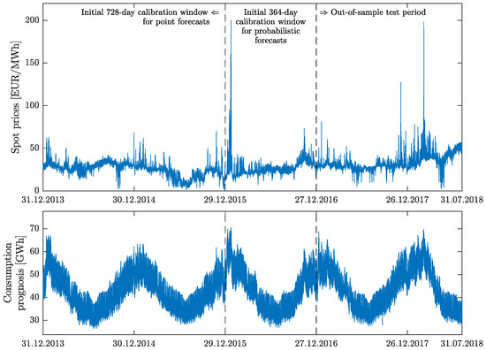
Figure 1.
Nord Pool (NP) hourly system prices (top) and hourly consumption prognosis (bottom) from 31 December 2013 to 31 July 2018. The first dashed line marks the beginning (29 December 2015) of the initial 364-day calibration window for probabilistic forecasts, the second—the beginning (27 December 2016) of the 582-day long out-of-sample test period.
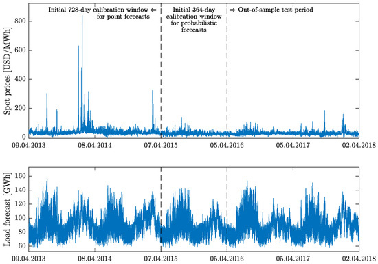
Figure 2.
PJM hourly system prices (top) and hourly load forecasts (bottom) in the Commonwealth Edison (COMED) zone from 9 April 2013 to 2 April 2018. The first dashed line marks the beginning (7 April 2015) of the initial 364-day calibration window for probabilistic forecasts, the second—the beginning (5 April 2016) of the 728-day long out-of-sample test period.
3. Methodology
3.1. The Forecasting Scheme
In our empirical study, we use a rolling window scheme. Every day we compute 24 predictive distributions for each of the 24 hours of the next day, then move the calibration windows forward by one day and repeat the exercise. The calibration windows for probabilistic predictions range between and 364 days, i.e., overall we consider 351 different window lengths. On the other hand, to obtain each predictive distribution we always use exactly six calibration windows for point forecasts: and 728 days.
Let us now illustrate this procedure using the Nord Pool dataset. To obtain predictive distributions for 27 December 2016 (denoted by an asterisk ‘*’ in Figure 3) using the longest calibration window for probabilistic forecasts ( days; the light red shaded bar in the top part of Figure 3) we apply the QRA and QRM approaches to point forecasts obtained for the period from 29 December 2015 to 26 December 2016, i.e., the initial 364-day calibration window for probabilistic forecasts, see Figure 1. Of course, before we can do this, we have to compute the point forecasts for 29 December 2015 to 26 December 2016 by fitting the ARX2 model to data in one of the six point forecasting calibration windows (blue shaded bars in the top part of Figure 3) directly preceding 29 December 2015, 30 December 2015, …, 26 December 2016. For instance, for we use data in the initial 728-day window (i.e., 31 December 2013 to 28 December 2015; light blue bar), while for in a 56-day window from 11 November 2015 to 28 December 2015 (dark blue bar).
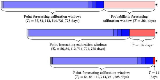
Figure 3.
Illustration of our forecasting scheme. The target day for which the predictive distributions are computed is denoted by an asterisk ‘*’. The calibration windows for probabilistic forecasts (red shaded bars; the darker the shade the shorter the window) end on the previous day. Here three windows are plotted: the longest considered ( days; top), an intermediate ( days; middle) and the shortest considered ( days; bottom). They are directly preceded by six calibration windows for point forecasts (blue shaded bars; the darker the shade the shorter the window) of and 728 days.
Similarly, to obtain predictive distributions for 27 December 2016 using the shortest calibration window for probabilistic forecasts ( days; the dark red shaded bar in the bottom part of Figure 3) we apply the QRA and QRM approaches to point forecasts obtained for the 14-day period from 13 to 26 December 2016. Again, before we can do this, we have to compute the point forecasts for 13 December 2016 to 26 December 2016 by fitting the ARX2 model to data in one of the six point forecasting calibration windows (blue shaded bars in the bottom part of Figure 3) directly preceding 13 December 2016, 14 December 2016, …, 26 December 2016.
3.2. Computing Point Forecasts
Our point forecasting setup directly mimics that of Marcjasz et al. [6]. In particular, our modeling is conducted within a ‘multivariate’ framework, where we explicitly use the ‘day × hour’ matrix-like structure with representing the electricity price for day d and hour h. We calibrate our model to transformed data, i.e., , where is the so-called variance stabilizing transformation (VST) [20]. In our case is the area hyperbolic sine:
where are ‘normalized’ prices, a is the median of in the (point forecasting) calibration window and b is the sample median absolute deviation (MAD) around the sample median adjusted by a factor for asymptotically normal consistency to the standard deviation. This factor is where is the 75% quantile of the normal distribution. After computing the forecasts, we apply the inverse transformation, the hyperbolic sine, i.e., , in order to obtain the price predictions:
For computing point forecasts we use the well-performing model of Ziel and Weron [21], only expanded to include one exogenous variable (consumption or load forecast; see the bottom panels in Figure 1 and Figure 2). Within this model, as in [6] denoted here by ARX2, the VST-transformed price on day d and hour h is given by:
where and are the minimum and the maximum of the previous day’s 24 hourly prices, is the previous day’s price at midnight (included in the model to take advantage of the influence it has on the prices for early morning hours [11,22]), is the known on day and VST-transformed consumption or load forecast for day d and hour h, and finally are weekday dummies which capture the short-term seasonality. As in [6], the model parameters, i.e., , are estimated using Ordinary Least Squares (OLS), independently for each hour .
3.3. Computing Probabilistic Forecasts
In this paper, we introduce two extensions of the averaging across calibration windows concept to probabilistic forecasting. The first one is based on Quantile Regression Averaging (QRA) of Nowotarski and Weron [7], which has been found to perform very well in several test cases, including electricity price [3,11,23,24], load [25,26,27] and wind power forecasting [28]. Recall, that QRA involves applying quantile regression [9] to a pool of point forecasts. More precisely, the q-th quantile of the predicted variable (here: the electricity price ) is represented by a linear combination of predictor variables:
where is a vector of weights for quantile q, estimated by minimizing the so-called pinball score for each quantile, see Section 4. In our case, the predictor (or explanatory) variables are the point forecasts obtained for the six considered calibration windows:
where denotes a vector of ones (i.e., the intercept) and a vector of point forecasts, obtained for the ARX2 model using one of the six calibration windows (i.e., or 728 days).
The second approach, after Marcjasz et al. [8] dubbed Quantile Regression Machine (QRM), first averages point predictions across the six calibration windows to yield , then applies quantile regression (4) to the combined forecast:
Note, that is of the same length as the six individual forecasts , hence the ‘argument’ T. The term Quantile Regression Machine is a compilation of ‘quantile regression’ and ‘committee machine’, since in [8] the authors considered committees of neural networks. Here, we use only regression models, but their weighted average across calibration windows reminds of the output of a committee machine. To reduce the complexity of our study we limit ourselves to the averaging scheme for point forecasts recommended by Marcjasz et al. [6], i.e., WAW(56:28:112, 714:7:728), which assigns weights based on yesterday’s performance of the ARX2 model in each calibration window, see Equation (5) in [6]. Regarding notation, recall from Section 3.1 that the calibration windows for probabilistic predictions range between and 364 days. We use QRA(T) to denote a QRA-type and QRM(T) to denote a QRM-type probabilistic forecast obtained for a window of length T.
Finally, note that both for QRA and QRM, for each day d and hour h we forecast 99 percentiles, i.e., , which approximate the entire predictive distribution relatively well. However, due to numerical inefficiency of quantile regression (4) the neighboring percentiles may be overlapping, leading to a phenomenon known as quantile crossing [29]. Hence, following Maciejowska and Nowotarski [11], the 99 quantiles are sorted to obtain monotonic quantile curves, independently for each day and hour.
3.4. Averaging Probabilistic Forecasts Across Calibration Windows
Given a set of probabilistic forecasts for calibration windows of days, we can combine all or some of them in one of two commonly used ways—by averaging probabilities or quantiles. The average quantile forecast, i.e., a horizontal average of the corresponding predictive distributions, is always more concentrated than the average probability forecast, i.e., a vertical average. While this feature is an advantage in many forecasting applications [15], it is not so in EPF [8,30]. Hence, in this study we only consider the average probability forecast defined as:
where is the i-th distributional forecast, actually a set of 99 percentiles obtained by setting in Equation (4), and n is the number of combined predictive distributions. We use this averaging scheme for both the QRA- and QRM-type probabilistic forecasts and respectively denote the combined forecasts by and , where is the vector of calibration windows used.
4. Results
We evaluate the probabilistic forecasts in terms of the Pinball Score, a so-called proper scoring rule and a special case of an asymmetric piecewise linear loss function [3,31]:
where is the forecast of the q-th quantile of obtained using Equation (4), is the observed price and q is the quantile. The lower the score is, the more accurate are the probabilistic forecasts, i.e., the more concentrated are the predictive distributions. Note, that Equation (8) measures the predictive accuracy for only one particular quantile. However, it can be averaged across all percentiles (i.e., ) and all hours in the whole out-of-sample test period to yield the Aggregate Pinball Score (APS). Note, that computing the APS is equivalent to computing the quantile representation of the Continuous Ranked Probability Score (CRPS) [32,33], i.e., it is a discretization of the CRPS, which replaces an integral over all quantiles by a simpler to compute sum over 99 percentiles [3].
4.1. QRA vs. QRM
Let us first compare the two approaches to computing probabilistic forecasts described in Section 3.3. In Figure 4 we plot the APS across all 99 percentiles and all hours in the 582-day (for Nord Pool) and 728-day (for PJM) out-of-sample test periods, see Figure 1 and Figure 2. Clearly, for each dataset and each T, QRM(T) yields more accurate probabilistic forecasts than QRA(T), with the results converging towards each other for larger windows. The latter may be due to too few observations for QRA to perform well for the shorter calibration windows, as it has 3.5 times more parameters to estimate than QRM. Given that computing predictive distributions via QRM is nearly three times faster than via QRA, we recommend the former approach. Note also, that initially we have considered calibration windows as short as 7 days. However, probabilistic forecasts for windows of less than 14 days perform poorly. For this reason they are not discussed in this paper.
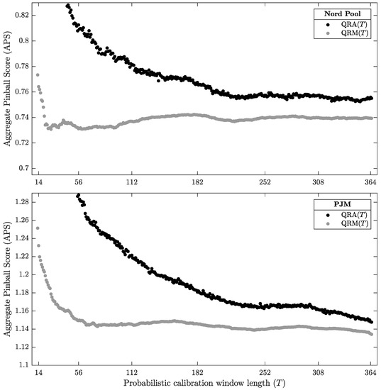
Figure 4.
Aggregate Pinball Scores (APS) for the Nord Pool (top) and PJM (bottom) datasets as a function of days.
4.2. Averaging Probabilistic Forecasts across Calibration Windows
Now, let us turn to the core part of this empirical study. Analogously to [5,6], we examine several different combinations of calibration windows for probabilistic EPF. The results are illustrated in Figure 5 (for Nord Pool) and Figure 6 (for PJM). We can observe that for both datasets QRA(14:7:364), i.e., the combination across all window lengths with a step of 7 days depicted in both Figures by green triangles, is a top performer among QRA-type predictions. QRM(14:7:364) also yields good forecasts, that are more accurate than QRM(T) for all T, but is in turn outperformed by more sparse sets of windows. In particular, QRA(14:7:28,308:28:364) denoted by black stars and QRA(14:28:70,308:28:364) denoted by dark red squares outperform all other combinations. In addition, they are computationally efficient—they require computing probabilistic forecasts for only six calibration windows. This reminds of the results for point forecasts [5,6], where also combinations of three short and three long windows were top performers.
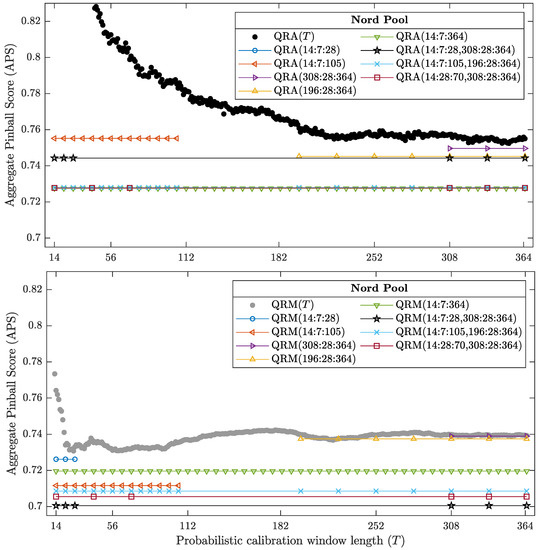
Figure 5.
Aggregate pinball scores (APS) for probabilistic QRA (top) and QRM (bottom) forecasts for the Nord Pool dataset. Filled circles refer to individual probabilistic calibration window lengths and lines with symbols indicate window lengths selected for averaging forecasts.
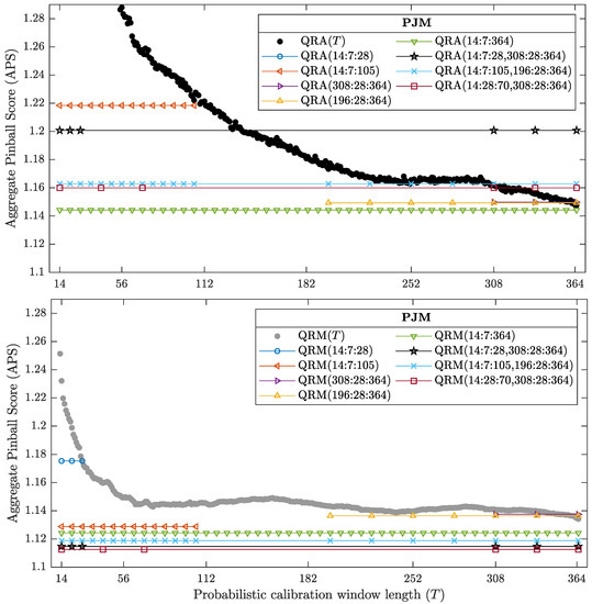
Figure 6.
Aggregate pinball scores (APS) for probabilistic QRA (top) and QRM (bottom) forecasts for the PJM dataset. Filled circles refer to individual probabilistic calibration window lengths and lines with symbols indicate window lengths selected for averaging forecasts.
4.3. The CPA Test and Statistical Significance
The analyzed so far Aggregate Pinball Scores (APS) can be used to provide a ranking, but do not allow drawing statistically significant conclusions on the outperformance of the forecasts of one window set by those of another. Therefore, we use the Giacomini and White [19] test for conditional predictive ability (CPA), which can be regarded as a generalization of the commonly used Diebold-Mariano test for unconditional predictive ability. Since only the CPA test accounts for parameter estimation uncertainty, it is the preferred option. Here, one statistic for each pair of window sets is computed based on the 24-dimensional vector of Pinball Scores for each day:
where for window set . For each pair of window sets and each dataset we compute the p-value of the CPA test with null in the regression [19]:
where contains elements from the information set on day , i.e., a constant and lags of .
In Figure 7 we illustrate the obtained p-values using ‘chessboards’, analogously as in [20,21,30,34] for the Diebold-Mariano test, i.e., we use a heat map to indicate the range of the p-values—the closer they are to zero (→ dark green) the more significant is the difference between the forecasts of a window set on the X-axis (better) and the forecasts of a window set on the Y-axis (worse). Evidently, the CPA test results confirm and emphasize the observations made in Section 4.2. In particular, QRM(14:7:28,308:28:364) and QRM(14:28:70,308:28:364) significantly outperform all other window sets; additionally for Nord Pool data QRM(14:7:28,308:28:364) is significantly more accurate than QRM(14:28:70,308:28:364). Comparing the averaging schemes, it is worth noting that in no case does QRA significantly outperform the corresponding QRM scheme. On the other hand, the opposite can be observed for several cases for both datasets. This result reinforces our recommendation of using the QRM scheme for probabilistic EPF, regardless of the number of predictions combined.
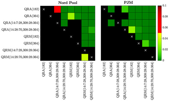
Figure 7.
Results of the conditional predictive ability (CPA) test [19] for forecasts of selected models for the Nord Pool (left) and PJM (right) data. We use a heat map to indicate the range of the p-values—the closer they are to zero (→ dark green) the more significant is the difference between the forecasts of a model on the X-axis (better) and the forecasts of a model on the Y-axis (worse).
5. Conclusions
In this paper, we take the averaging across calibration windows concept to a new level. Motivated by the results of Hubicka et al. [5] and Marcjasz et al. [6] for point forecasts, we consider two extensions of this approach to probabilistic forecasting: one based on Quantile Regression Averaging (QRA) [7], the other on the Quantile Regression Machine (QRM) [8]. Both methods apply quantile regression to a pool of point forecasts in order to obtain predictions for the 99 percentiles of the next day’s price distribution. The difference between them lies in the choice of the regressors—QRA uses the point forecasts themselves, while QRM the combined point forecast.
Somewhat surprisingly, it turns out that it is not only more computationally efficient, but also better in terms of the Pinball Score to first average point predictions and then apply quantile regression to the combined forecast, than to use quantile regression directly on the individual point forecasts. In other words, a more general approach (QRA) is outperformed by a two-step technique (QRM). We believe that this outcome is due to two factors: the simpler model structure with fewer parameters to estimate and the more accurate point forecasts used as inputs. As Uniejewski et al. [30] have recently shown, more accurate point forecasts directly translate into better probabilistic forecasts computed via quantile regression. In addition, averaging point forecasts for a few adequately chosen calibration window lengths leads to decreasing the MAE by about 5% compared to the best point forecast obtained for a single window, even selected ex-post [5,6].
Regarding the selection of calibration windows for combining forecasts, similarly to the results for point predictions, the best performing combinations are those averaging a small number of short- and long-term windows. In particular, QRM(14:7:28,308:28:364) significantly outperforms all other considered window sets and is recommended for averaging probabilistic forecasts. We should emphasize that in this study we are using only one, relatively simple way of combining probabilistic forecasts, i.e., the average probability forecast, but the literature on combining predictive distributions offers interesting alternatives [15,16,17,18]. They could be tested in this context as well. Moreover, the proposed methodology can be easily extended to other areas of energy forecasting (e.g., load, solar, wind) or other types of markets (e.g., intraday). Finally, the economic benefits from using more accurate probabilistic electricity price predictions could be evaluated, as is becoming more common in the point forecasting literature [35,36].
Author Contributions
Conceptualization, R.W.; Investigation, T.S. and B.U.; Software, T.S. and B.U.; Validation, R.W.; Writing—original draft, T.S. and B.U.; Writing—review & editing, R.W.
Funding
This work was partially supported by the National Science Center (NCN, Poland) through grant No. 2015/17/B/HS4/00334 (to T.S. and R.W.) and No. 2016/23/G/HS4/01005 (to B.U.).
Conflicts of Interest
The authors declare no conflict of interest.
References
- Weron, R. Electricity price forecasting: A review of the state-of-the-art with a look into the future. Int. J. Forecast. 2014, 30, 1030–1081. [Google Scholar] [CrossRef]
- Lago, J.; De Ridder, F.; De Schutter, B. Forecasting spot electricity prices: Deep learning approaches and empirical comparison of traditional algorithms. Appl. Energy 2018, 221, 386–405. [Google Scholar] [CrossRef]
- Nowotarski, J.; Weron, R. Recent advances in electricity price forecasting: A review of probabilistic forecasting. Renew. Sustain. Energy Rev. 2018, 81, 1548–1568. [Google Scholar] [CrossRef]
- Ziel, F.; Steinert, R. Probabilistic mid- and long-term electricity price forecasting. Renew. Sustain. Energy Rev. 2018, 94, 251–266. [Google Scholar] [CrossRef]
- Hubicka, K.; Marcjasz, G.; Weron, R. A note on averaging day-ahead electricity price forecasts across calibration windows. IEEE Trans. Sustain. Energy 2019, 10, 321–323. [Google Scholar] [CrossRef]
- Marcjasz, G.; Serafin, T.; Weron, R. Selection of calibration windows for day-ahead electricity price forecasting. Energies 2018, 11, 2364. [Google Scholar] [CrossRef]
- Nowotarski, J.; Weron, R. Computing electricity spot price prediction intervals using quantile regression and forecast averaging. Comput. Stat. 2015, 30, 791–803. [Google Scholar] [CrossRef]
- Marcjasz, G.; Uniejewski, B.; Weron, R. Probabilistic electricity price forecasting with NARX networks: Combine point or probabilistic forecasts? Int. J. Forecast. 2019. forthcoming. [Google Scholar]
- Koenker, R.W. Quantile Regression; Cambridge University Press: Cambridge, UK, 2005. [Google Scholar]
- Juban, R.; Ohlsson, H.; Maasoumy, M.; Poirier, L.; Kolter, J. A multiple quantile regression approach to the wind, solar, and price tracks of GEFCom2014. Int. J. Forecast. 2016, 32, 1094–1102. [Google Scholar] [CrossRef]
- Maciejowska, K.; Nowotarski, J. A hybrid model for GEFCom2014 probabilistic electricity price forecasting. Int. J. Forecast. 2016, 32, 1051–1056. [Google Scholar] [CrossRef]
- Andrade, J.; Filipe, J.; Reis, M.; Bessa, R. Probabilistic price forecasting for day-ahead and intraday markets: Beyond the statistical model. Sustainability 2017, 9, 1990. [Google Scholar] [CrossRef]
- Bracale, A.; Carpinelli, G.; De Falco, P. Developing and comparing different strategies for combining probabilistic photovoltaic power forecasts in an ensemble method. Energies 2019, 12, 1011. [Google Scholar] [CrossRef]
- Ziel, F. Quantile regression for the qualifying match of GEFCom2017 probabilistic load forecasting. Int. J. Forecast. 2019. [Google Scholar] [CrossRef]
- Lichtendahl, K.C.; Grushka-Cockayne, Y.; Winkler, R.L. Is it better to average probabilities or quantiles? Manag. Sci. 2013, 59, 1594–1611. [Google Scholar] [CrossRef]
- Gneiting, T.; Ranjan, R. Combining predictive distributions. Electron. J. Stat. 2013, 7, 1747–1782. [Google Scholar] [CrossRef]
- Bassetti, F.; Casarin, R.; Ravazzolo, F. Bayesian nonparametric calibration and combination of predictive distributions. J. Am. Stat. Assoc. 2018, 113, 675–685. [Google Scholar] [CrossRef]
- Baran, S.; Lerch, S. Combining predictive distributions for the statistical post-processing of ensemble forecasts. Int. J. Forecast. 2018, 34, 477–496. [Google Scholar] [CrossRef]
- Giacomini, R.; White, H. Tests of conditional predictive ability. Econometrica 2006, 74, 1545–1578. [Google Scholar] [CrossRef]
- Uniejewski, B.; Weron, R.; Ziel, F. Variance stabilizing transformations for electricity spot price forecasting. IEEE Trans. Power Syst. 2018, 33, 2219–2229. [Google Scholar] [CrossRef]
- Ziel, F.; Weron, R. Day-ahead electricity price forecasting with high-dimensional structures: Univariate vs. multivariate modeling frameworks. Energy Econ. 2018, 70, 396–420. [Google Scholar] [CrossRef]
- Ziel, F. Forecasting electricity spot prices using LASSO: On capturing the autoregressive intraday structure. IEEE Trans. Power Syst. 2016, 31, 4977–4987. [Google Scholar] [CrossRef]
- Gaillard, P.; Goude, Y.; Nedellec, R. Additive models and robust aggregation for GEFCom2014 probabilistic electric load and electricity price forecasting. Int. J. Forecast. 2016, 32, 1038–1050. [Google Scholar] [CrossRef]
- Kostrzewski, M.; Kostrzewska, J. Probabilistic electricity price forecasting with Bayesian stochastic volatility models. Energy Econ. 2019, 80, 610–620. [Google Scholar] [CrossRef]
- Liu, B.; Nowotarski, J.; Hong, T.; Weron, R. Probabilistic load forecasting via Quantile Regression Averaging on sister forecasts. IEEE Trans. Smart Grid 2017, 8, 730–737. [Google Scholar] [CrossRef]
- Sigauke, C.; Nemukula, M.; Maposa, D. Probabilistic hourly load forecasting using additive quantile regression models. Energies 2018, 11, 2208. [Google Scholar] [CrossRef]
- Wang, Y.; Zhang, N.; Tan, Y.; Hong, T.; Kirschen, D.; Kang, C. Combining probabilistic load forecasts. IEEE Trans. Smart Grid 2019. [Google Scholar] [CrossRef]
- Zhang, Y.; Liu, K.; Qin, L.; An, X. Deterministic and probabilistic interval prediction for short-term wind power generation based on variational mode decomposition and machine learning methods. Energy Convers. Manag. 2016, 112, 208–219. [Google Scholar] [CrossRef]
- Chernozhukov, V.; Fernandez-Val, I.; Galichon, A. Quantile and probability curves without crossing. Econometrica 2010, 73, 1093–1125. [Google Scholar]
- Uniejewski, B.; Marcjasz, G.; Weron, R. On the importance of the long-term seasonal component in day-ahead electricity price forecasting. Part II—Probabilistic forecasting. Energy Econ. 2019, 79, 171–182. [Google Scholar] [CrossRef]
- Gneiting, T. Quantiles as optimal point forecasts. Int. J. Forecast. 2011, 27, 197–207. [Google Scholar] [CrossRef]
- Gneiting, T.; Ranjan, R. Comparing density forecasts using thresholdand quantile-weighted scoring rules. J. Bus. Econ. Stat. 2011, 29, 411–422. [Google Scholar] [CrossRef]
- Laio, F.; Tamea, S. Verification tools for probabilistic forecasts of continuous hydrological variables. Hydrol. Earth Syst. Sci. 2007, 11, 1267–1277. [Google Scholar] [CrossRef]
- Uniejewski, B.; Weron, R. Efficient forecasting of electricity spot prices with expert and LASSO models. Energies 2018, 11, 2039. [Google Scholar] [CrossRef]
- Kath, C.; Ziel, F. The value of forecasts: Quantifying the economic gains of accurate quarter-hourly electricity price forecasts. Energy Econ. 2018, 76, 411–423. [Google Scholar] [CrossRef]
- Maciejowska, K.; Nitka, W.; Weron, T. Day-ahead vs. Intraday—Forecasting the price spread to maximize economic benefits. Energies 2019, 12, 631. [Google Scholar] [CrossRef]


© 2019 by the authors. Licensee MDPI, Basel, Switzerland. This article is an open access article distributed under the terms and conditions of the Creative Commons Attribution (CC BY) license (http://creativecommons.org/licenses/by/4.0/).