Article

Comprehensive Second-Order Adjoint Sensitivity Analysis Methodology (2nd-ASAM) Applied to a Subcritical Experimental Reactor Physics Benchmark: II. Effects of Imprecisely Known Microscopic Scattering Cross Sections

Center for Nuclear Science and Energy, Department of Mechanical Engineering, University of South Carolina, Columbia, SC 29208, USA
*
Author to whom correspondence should be addressed.
Energies 2019, 12(21), 4114; https://doi.org/10.3390/en12214114
Submission received: 27 August 2019 / Revised: 21 October 2019 / Accepted: 23 October 2019 / Published: 28 October 2019

Abstract

:
This work continues the presentation commenced in Part I of the second-order sensitivity analysis of nuclear data of a polyethylene-reflected plutonium (PERP) benchmark using the Second-Order Adjoint Sensitivity Analysis Methodology (2nd-ASAM). This work reports the results of the computations of the first- and second-order sensitivities of this benchmark’s computed leakage response with respect to the benchmark’s 21,600 parameters underlying the computed group-averaged isotopic scattering cross sections. The numerical results obtained for the 21,600 first-order relative sensitivities indicate that the majority of these were small, the largest having relative values of O (10−2). Furthermore, the vast majority of the (21600)2 second-order sensitivities with respect to the scattering cross sections were much smaller than the corresponding first-order ones. Consequently, this work shows that the effects of variances in the scattering cross sections on the expected value, variance, and skewness of the response distribution were negligible in comparison to the corresponding effects stemming from uncertainties in the total cross sections, which were presented in Part I. On the other hand, it was found that 52 of the 21600 × 180 mixed second-order sensitivities of the leakage response with respect to the scattering and total microscopic cross sections had values that were significantly larger than the unmixed second-order sensitivities of the leakage response with respect to the group-averaged scattering microscopic cross sections. The first- and second-order mixed sensitivities of the PERP benchmark’s leakage response with respect to the scattering cross sections and the other benchmark parameters (fission cross sections, average number of neutrons per fission, fission spectrum, isotopic atomic number densities, and source parameters) have also been computed and will be reported in subsequent works.

1. Introduction

In continuation of the results presented in Part I [1], this work presents the numerical results for the first- and second-order sensitivities of the leakage response of the polyethylene-reflected plutonium (PERP) benchmark described in [2] with respect to the benchmark’s group-averaged isotopic scattering cross sections. This work also presents the results for the mixed second-order sensitivities to both the scattering and total cross sections. As has been described in Part I [1], the numerical model of the PERP benchmark includes 180 ( J σ t = I × G ) imprecisely-known parameters for the group-averaged total microscopic cross sections and 21,600 ( J σ s = ( G × G ) × I × ( I S C T + 1 ) ) imprecisely-known parameters for group-averaged scattering microscopic cross sections, where I = 6 , G = 30 and I S C T = 3 are the number of isotopes, energy groups and Legendre expansion orders for the PERP benchmark, respectively. Therefore, there are 21,600 first-order sensitivities, 21600 × 21600 second-order sensitivities of the PERP benchmark’s leakage response to the group-averaged microscopic scattering cross sections, and 21600 × 180 mixed second-order sensitivities to the scattering and total microscopic cross sections. These sensitivities will be computed by specializing the general expressions derived by Cacuci [3] to the PERP benchmark. Section 2 of this work presents computational results for the first- and second-order sensitivities of the PERP benchmark’s leakage response with respect to the group-averaged microscopic scattering cross sections. Section 3 reports the numerical results for the matrix of mixed second-order leakage sensitivities to the group-averaged total and scattering microscopic cross sections. Section 4 presents the impact of the first- and second-order sensitivities on the uncertainties induced for the leakage response by the imprecisely-known group-averaged scattering microscopic cross section. Section 5 concludes this work. The computational results for the sensitivities of the PERP leakage response to the remaining imprecisely-known model parameters (fission cross sections and number of neutrons produced per fission, fission spectra, and isotopic number densities) will be reported in subsequent publications.

2. Computation of First- and Second-Order Sensitivities of the PERP Leakage Response to Scattering Cross Sections

The physical system considered in this work is the same polyethylene-reflected plutonium (acronym that will be used in this work: PERP) metal sphere benchmark [2] as described in Part I [1]. As in Part I [1], the neutron flux is computed by solving numerically the neutron transport equation using the PARTISN [4] multigroup discrete ordinates transport code. For the PERP benchmark under consideration, PARTISN [4] solves the following multi-group approximation of the neutron transport equation with a spontaneous fission source provided by the code SOURCES4C [5]:
B g ( α ) φ g ( r , Ω ) = Q g ( r ) , g = 1 , , G ,
φ g ( r d , Ω ) = 0 , r d S b , Ω n < 0 , g = 1 , , G ,
where
B g ( α ) φ g ( r , Ω ) Ω · φ g ( r , Ω ) + Σ t g ( r ) φ g ( r , Ω ) g = 1 G 4 π Σ s g g ( r , Ω Ω ) φ g ( r , Ω ) d Ω χ g ( r ) g = 1 G 4 π ( ν Σ ) f g ( r ) φ g ( r , Ω ) d Ω ;
Q g ( r ) k = 1 N f λ k N k , 1 F k S F ν k S F e E g / a k sinh b k E g , g = 1 , , G ,
and where α denotes the “vector of imprecisely-known model parameters”, as defined in Part I [1].
The PARTISN [4] calculations used MENDF71X 618-group cross sections [6] collapsed to G = 30 energy groups, with group boundaries, E g , as presented in Part I [1]. The MENDF71X library uses ENDF/B-VII.1 Nuclear Data [7]. As has been discussed in [1], the fundamental quantities (i.e., system responses) of interest for subcritical benchmarks (such as the PERP benchmark) are singles counting rate, doubles counting rate, the leakage multiplication, and the total leakage. The total leakage is physically more meaningful than count rates because it does not depend on the detector configuration. For this reason, many systems are characterized for practical applications by their total leakage rather than by the count rate that a particular detector would see at a particular distance. For this reason, this work considers the total leakage from the PERP benchmark to be the paradigm response of interest for sensitivity analysis; sensitivities analyses of counting rates and other responses can be performed in an analogous manner, i.e., by following the general ideas that will be presented in this work (and in subsequent related works).
Mathematically, the total neutron leakage from the PERP sphere, denoted as L ( α ) , will depend (indirectly, through the neutron flux) on all of the imprecisely-known model parameters and is defined as follows:
L ( α ) S b d S g = 1 G Ω n > 0 d Ω Ω n φ g ( r , Ω ) .
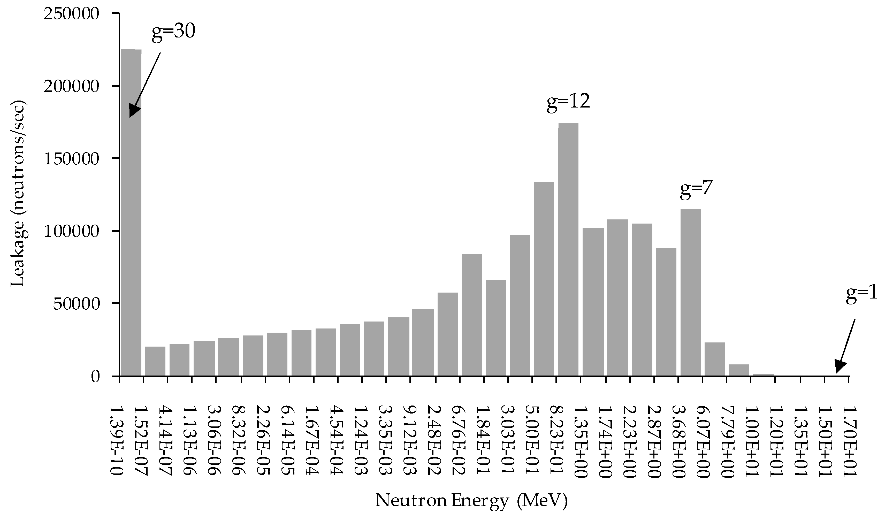
Figure 1 shows the histogram plot of the leakage for each energy group for the PERP benchmark. The total leakage computed using Equation (5) for the PERP benchmark is 1.7648 × 10 6 neutrons/sec.
The scattering transfer cross section Σ s g g ( r , Ω Ω ) from energy group g , g = 1 , , G into energy group g , g = 1 , , G , is computed in terms of the l -th order Legendre coefficient σ s , l , i g g , of the Legendre-expanded microscopic scattering cross section from energy group g into energy group g for isotope i . Since the cross-sections for every material are treated in the PARTISN [4] calculations as being space-independent within the respective material, the variable r will henceforth no longer appear in the arguments of the various cross sections. The coefficients σ s , l , i g g are tabulated parameters, and the finite-order Legendre-expansion of Σ s g g ( Ω Ω ) has the following expression:
Σ s g g ( Ω Ω ) = m = 1 M = 2 Σ s , m g g ( Ω Ω ) , Σ s , m g g ( Ω Ω ) i = 1 I = 6 N i , m l = 0 I S C T = 3 ( 2 l + 1 ) σ s , l , i g g P l ( Ω Ω ) , m = 1 , 2 ,
where I S C T = 3 denotes the order of the respective finite expansion in Legendre polynomial.
The total cross section Σ t g for energy group g , g = 1 , , G , and material m is computed for the PERP benchmark using the following expression:
Σ t g = m = 1 M = 2 Σ t , m g ; Σ t , m g = i I N i , m σ t , i g = i I N i , m [ σ f , i g + σ c , i g + g = 1 G σ s , l = 0 , i g g ] , m = 1 , 2 ,
where σ f , i g and σ c , i g denote, respectively, the tabulated group microscopic fission and neutron capture cross sections for group g , g = 1 , , G . Other nuclear reactions, including (n,2n) and (n,3n) reactions are not present in the PERP benchmark. The expressions in Equations (6) and (7) indicate that the zeroth order (i.e., l = 0 ) scattering cross sections must be considered separately from the higher order (i.e., l 1 ) scattering cross sections, since the l = 0 scattering cross sections contribute to the total cross sections, while the l 1 scattering cross sections do not contribute to the total cross sections.
As discussed in Part I [1], the total cross section Σ t g Σ t g ( t ) will depend on the vector of parameter t , which is defined as follows:
t [ t 1 , , t J t ] [ t 1 , , t J σ t ; n 1 , , n J n ] [ σ t ; N ] , J t = J σ t + J n ,
where
N [ n 1 , , n J n ] [ N 1 , 1 , N 2 , 1 , N 3 , 1 , N 4 , 1 , N 5 , 2 , N 6 , 2 ] , J n = 6 .
σ t [ t 1 , , t J σ t ] [ σ t , i = 1 1 , σ t , i = 1 2 , , σ t , i = 1 G , , σ t , i g , , σ t , i = I 1 , , σ t , i = I G ] , i = 1 , , I ; g = 1 , , G ; J σ t = I × G .
In Equations (8)–(10), the dagger denotes “transposition,” σ t , i g denotes the microscopic total cross section for isotope i and energy group g , N i , m denotes the respective isotopic number density, and J n denotes the total number of isotopic number densities in the model. Thus, the vector t comprises a total of J t = J σ t + J n = 30 × 6 + 6 = 186 imprecisely-known “model parameters” as its components.
In view of Equation. (6), the scattering cross section Σ s g g ( Ω Ω ) Σ s g g ( s ; Ω Ω ) depends on the vector of parameters s , which is defined as follows:
s [ s 1 , , s J s ] [ s 1 , , s J σ s ; n 1 , , n J n ] [ σ s ; N ] , J s = J σ s + J n ,
σ s [ s 1 , , s J σ s ] [ σ s , l = 0 , i = 1 g = 1 g = 1 , σ s , l = 0 , i = 1 g = 2 g = 1 , , σ s , l = 0 , i = 1 g = G g = 1 , σ s , l = 0 , i = 1 g = 1 g = 2 , σ s , l = 0 , i = 1 g = 2 g = 2 , , σ s , l , i g g , , σ s , I S C T , i = I G G ] , l = 0 , , I S C T ; i = 1 , , I ; g , g = 1 , , G ; J σ s = ( G × G ) × I × ( I S C T + 1 ) .
As stated above, the zeroth order (i.e., l = 0 ) scattering cross sections need to be separately considered from the higher order (i.e., l 1 ) ones. Therefore, in σ s , the total number of zeroth order scattering cross section is denoted as J σ s , l = 0 , where J σ s , l = 0 = G × G × I ; and the total number of higher order (i.e., l 1 ) scattering cross sections is denoted as J σ s , l 1 , where J σ s , l 1 = G × G × I × I S C T , with J σ s , l = 0 + J σ s , l 1 = J σ s . The vector s comprises a total of J σ s + J n = 30 × 30 × 6 × ( 3 + 1 ) + 6 = 21606 imprecisely-known components (“model parameters”).
Recall from Part I [1] that the components of the vector of first-order sensitivities of the leakage response with respect to the model parameters are denoted as S ( 1 ) ( α ) , which is defined as follows:
S ( 1 ) ( α ) [ L ( α ) σ t ; L ( α ) σ s ; L ( α ) σ f ; L ( α ) ν ; L ( α ) p ; L ( α ) q ; L ( α ) N ] .
The symmetric matrix of second-order sensitivities of the leakage response with respect to the model parameters is denoted as S ( 2 ) ( α ) , and is defined as follows:
S ( 2 ) ( α ) [ 2 L ( α ) σ t σ t 2 L ( α ) σ s σ t 2 L ( α ) σ s σ s 2 L ( α ) σ f σ t 2 L ( α ) σ f σ s 2 L ( α ) σ f σ f 2 L ( α ) ν σ t 2 L ( α ) ν σ s 2 L ( α ) ν σ f 2 L ( α ) ν ν 2 L ( α ) p σ t 2 L ( α ) p σ s 2 L ( α ) p σ f 2 L ( α ) p ν 2 L ( α ) p p 2 L ( α ) q σ t 2 L ( α ) q σ s 2 L ( α ) q σ f 2 L ( α ) q ν 2 L ( α ) q p 2 L ( α ) q q 2 L ( α ) N σ t 2 L ( α ) N σ s 2 L ( α ) N σ f 2 L ( α ) N ν 2 L ( α ) N p 2 L ( α ) N q 2 L ( α ) N N ] .
The results as well as their impact on the uncertainties induced in the leakage response by the first- and second-order sensitivities L ( α ) / σ t and, respectively, 2 L ( α ) / σ t σ t , were reported in Part I [1]. This work will report the computational results for the first-order sensitivities L ( α ) / σ s and the second-order sensitivities 2 L ( α ) / σ s σ s and 2 L ( α ) / σ s σ t , along with their effects on the uncertainties induced in the leakage response.

2.1. First-Order Sensitivities L ( α ) / σ s

The equations needed for deriving the expressions of the first-order sensitivities of L / s j , j = 1 , , J σ s will differ from each other depending on whether the parameters s j correspond to the zeroth-order ( l = 0 ) or to the higher order ( l 1 ) scattering cross sections. There are two distinct cases, as follows:
(1) ( L ( α ) s j ) ( s = σ s , l = 0 ) , j = 1 , , J σ s , l = 0 , where the quantities s j refer to the parameters underlying the zeroth-order scattering microscopic cross sections; and
(2) ( L ( α ) s j ) ( s = σ s , l 1 ) , j = 1 , , J σ s , l 1 , where the quantities s j refer to the parameters underlying the l t h -order ( l 1 ) scattering microscopic cross sections.

2.1.1. First-Order Sensitivities ( L ( α ) s j ) ( s = σ s , l = 0 ) , j = 1 , , J σ s , l = 0

The first-order sensitivities of the leakage response with respect to zeroth-order scattering microscopic cross sections are computed by particularizing Equations (150) and (151) in [3], where Equation (151) provides the contributions arising directly from the scattering cross sections, while Equation (150) provides contributions arising indirectly through the total cross sections. The expression obtained by particularizing Equation (151) in [3] to the PERP benchmark yields:
( L ( α ) s j ) ( s = σ s , l = 0 ) ( 1 ) = g = 1 G V d V 4 π d Ω ψ ( 1 ) , g ( r , Ω ) g = 1 G 4 π d Ω Σ s g g ( s ; Ω Ω ) s j φ g ( r , Ω ) , f o r j = 1 , , J σ s , l = 0 ,
where the multigroup adjoint fluxes ψ ( 1 ) , g ( r , Ω ) , g = 1 , , G are the solutions of the following first-Level Adjoint Sensitivity System (1st-LASS) presented in Equations (156) and (157) in [3]:
A ( 1 ) , g ( α ) ψ ( 1 ) , g ( r , Ω ) = Ω n δ ( r r d ) , g = 1 , , G ,
ψ ( 1 ) , g ( r d , Ω ) = 0 , Ω n > 0 , g = 1 , , G ,
where r d is the radius of the PERP sphere, and where the adjoint operator A ( 1 ) , g ( α ) takes on the following particular form of Equation (149) in [3]:
A ( 1 ) , g ( α ) ψ ( 1 ) , g ( r , Ω ) Ω · ψ ( 1 ) , g ( r , Ω ) + Σ t g ( t ; r ) ψ ( 1 ) , g ( r , Ω ) g = 1 G 4 π d Ω Σ s g g ( s ; r , Ω Ω ) ψ ( 1 ) , g ( r , Ω ) ν Σ f g ( f ; r ) g = 1 G 4 π d Ω χ g ( p ; r ) ψ ( 1 ) , g ( r , Ω ) , g = 1 , , G .
The contributions stemming from the total cross sections are computed using Equation (150) in [3] in conjunction with the relations L t j t j s j = L s j and Σ t g ( t ) t j t j s j = Σ t g ( t ) s j to obtain:
( L ( α ) s j ) ( s = σ s , l = 0 ) ( 2 ) = g = 1 G V d V 4 π d Ω ψ ( 1 ) , g ( r , Ω ) φ g ( r , Ω ) Σ t g ( t ) s j , j = 1 , , J σ s , l = 0 .
Adding Equations (13) and (17) yields the following complete expression:
( L ( α ) s j ) ( s = σ s , l = 0 ) = ( L ( α ) s j ) ( s = σ s , l = 0 ) ( 1 ) + ( L ( α ) s j ) ( s = σ s , l = 0 ) ( 2 ) = g = 1 G V d V 4 π d Ω ψ ( 1 ) , g ( r , Ω ) g = 1 G 4 π d Ω Σ s g g ( s ; Ω Ω ) s j φ g ( r , Ω ) g = 1 G V d V 4 π d Ω ψ ( 1 ) , g ( r , Ω ) φ g ( r , Ω ) Σ t g ( t ) s j , f o r j = 1 , , J σ s , l = 0 .
For the PERP benchmark, when the parameters s j correspond to the zeroth-order scattering microscopic cross sections, i.e., s j σ s , l j = 0 , i j g j g j , the following relations hold:
Σ s g g ( s ; Ω Ω ) s j = Σ s g g ( s ; Ω Ω ) σ s , l j , i j g j g j = [ m = 1 M i = 1 I N i , m σ s , i g g ( s ; Ω Ω ) ] σ s , l j , i j g j g j = [ m = 1 M i = 1 I l = 0 I S C T N i , m ( 2 l + 1 ) σ s , l , i g g P l ( Ω Ω ) ] σ s , l j , i j g j g j = δ g j g δ g j g N i j , m j ( 2 l j + 1 ) P l j ( Ω Ω ) ,
Σ t g ( t ) s j = [ m = 1 M i = 1 I N i , m σ t , i g ( t ) ] σ s , l j = 0 , i j g j g j = { m = 1 M i = 1 I N i , m [ σ f , i g ( f ) + σ c , i g ( c ) + g = 1 G σ s , l = 0 , i g g ( s ) ] } σ s , l j = 0 , i j g j g j = [ m = 1 M i = 1 I g = 1 G N i , m σ s , l = 0 , i g g ( s ) ] σ s , l j = 0 , i j g j g j = δ g j g N i j , m j ,
where the subscripts i j , l j , g j , g j and m j refer to the isotope, order of Legendre expansion, energy groups, and material associated with the parameter s j , respectively, and where δ g j g and δ g j g denote the Kronecker-delta functionals (e.g., δ g j g = 1 if g j = g ; δ g j g = 0 if g j g ). Inserting Equations (19) and (20) into Equation (18), using the addition theorem for spherical harmonics in one-dimensional geometry, performing the respective angular integrations, and finally setting l j = 0 in the resulting expression yields the following expression:
( L ( α ) s j ) ( s = σ s , l = 0 ) = N i j , m j V d V φ 0 g j ( r ) ξ 0 ( 1 ) , g j ( r ) N i j , m j V d V 4 π d Ω ψ ( 1 ) , g j ( r , Ω ) φ g j ( r , Ω ) , f o r j = 1 , , J σ s , l = 0 ,
where the forward and adjoint flux moments φ 0 g j ( r ) and ξ 0 ( 1 ) , g j ( r ) are defined as follows:
φ 0 g ( r ) 4 π d Ω φ g ( r , Ω ) ,
ξ 0 ( 1 ) , g ( r ) 4 π d Ω ψ ( 1 ) , g ( r , Ω ) .

2.1.2. First-Order Sensitivities ( L ( α ) s j ) ( s = σ s , l 1 ) , j = 1 , , σ s , l 1

The first-order sensitivities of the leakage response with respect to the l t h -order ( l 1 ) microscopic scattering cross sections are computed by particularizing Equation (151) in [3]:
( L ( α ) s j ) ( s = σ s , l 1 ) = g = 1 G V d V 4 π d Ω ψ ( 1 ) , g ( r , Ω ) g = 1 G 4 π d Ω Σ s g g ( s ; Ω Ω ) s j φ g ( r , Ω ) , f o r j = 1 , , σ s , l 1 .
Inserting Equation (19) into Equation (24), using the addition theorem for spherical harmonics in one-dimensional geometry and performing the respective angular integrations, yields the following expression:
( L ( α ) s j ) ( s = σ s , l 1 ) = N i j , m j ( 2 l j + 1 ) V d V φ l j g j ( r ) ξ l j ( 1 ) , g j ( r ) , j = 1 , , J σ s , l 1 ,
where the forward and adjoint flux moments φ l j g j ( r ) and ξ l j ( 1 ) , g j ( r ) are defined as follows:
φ l g ( r ) 4 π d Ω P l ( Ω ) φ g ( r , Ω ) ,
ξ l ( 1 ) , g ( r ) 4 π d Ω P l ( Ω ) ψ ( 1 ) , g ( r , Ω ) .
The numerical values of the first-order relative sensitivities, S ( 1 ) ( σ s , l = 0 , i g g ) ( L / σ s , l = 0 , i g g ) ( σ s , l = 0 , i g g / L ) , i = 1 , , 6 ; g = 1 , , 30 , of the leakage response with respect to the zeroth-order self-scattering microscopic cross sections for the six isotopes contained in the PERP benchmark will be presented in Section 2.3, in tables that will also include comparisons with the numerical values of the corresponding second-order unmixed relative sensitivities S ( 2 ) ( σ s , l = 0 , i g g , σ s , l = 0 , i g g ) ( 2 L / σ s , l = 0 , i g g σ s , l = 0 , i g g ) ( σ s , l = 0 , i g g σ s , l = 0 , i g g / L ) , i = 1 , , 6 ; g = 1 , , 30 .

2.2. Second-Order Sensitivities 2 L ( α ) / σ s σ s

As has already been mentioned, it is important to note that the equations needed for deriving the expressions of the second-order sensitivities of 2 L / s j s m 2 , j = 1 , , J σ s ; m 2 = 1 , , J σ s will differ from each other depending on whether the parameters s j and s m 2 correspond to the zeroth-order ( l = 0 ) or to the higher order ( l 1 ) scattering cross sections. There are four distinct cases, which will be presented in this Section’s four sub-sections, as follows:
A. ( 2 L s j s m 2 ) ( s = σ s , l = 0 , s = σ s , l = 0 ) , j = 1 , , J σ s , l = 0 ; m 2 = 1 , , J σ s , l = 0 , where both parameters s j and s m 2 correspond to the zeroth-order scattering cross sections;
B. ( 2 L s j s m 2 ) ( s = σ s , l = 0 , s = σ s , l 1 ) , j = 1 , , J σ s , l = 0 ; m 2 = 1 , , J σ s , l 1 , where parameters s j correspond to the zeroth-order scattering cross sections, and s m 2 correspond to the l t h -order ( l 1 ) scattering cross sections;
C. ( 2 L s j s m 2 ) ( s = σ s , l 1 , s = σ s , l = 0 ) , j = 1 , , J s , l 1 ; m 2 = 1 , , J s , l = 0 , where parameters s j correspond to the l t h -order ( l 1 ) scattering cross sections, and s m 2 correspond to the zeroth-order scattering cross sections;
D. ( 2 L s j s m 2 ) ( s = σ s , l 1 , s = σ s , l 1 ) , j = 1 , , J σ s , l 1 ; m 2 = 1 , , J σ s , l 1 , where both parameters s j and s m 2 correspond to the l t h -order ( l 1 ) scattering cross sections.

2.2.1. Second-Order Sensitivities ( 2 L s j s m 2 ) ( s = σ s , l = 0 , s = σ s , l = 0 ) , j = 1 , , J σ s , l = 0 ; m 2 = 1 , , J σ s , l = 0

For this case, both parameters s j and s m 2 correspond to the zeroth-order scattering cross sections, and are therefore denoted as s j σ s , l j = 0 , i j g j g j and s m 2 σ s , l m 2 = 0 , i m 2 g m 2 g m 2 , respectively. The subscripts i m 2 , l m 2 , g m 2 and g m 2 refer to the isotope, order of Legendre expansion, and energy groups associated with the parameter s m 2 , respectively. When both parameters s j σ s , l j = 0 , i j g j g j and s m 2 σ s , l m 2 = 0 , i m 2 g m 2 g m 2 correspond to the zeroth-order scattering cross sections, the expression of ( 2 L s j s m 2 ) ( s = σ s , l = 0 , s = σ s , l = 0 ) must include the respective contributions stemming from the total cross sections, since the definition of the total cross sections comprises the zeroth-order scattering cross sections. The contributions from the total cross section due to the zeroth-order scattering cross section parameters s j and s m 2 are computed using Equation (158) in [3] in conjunction with the relations 2 L t j t m 2 t j s j t m 2 s m 2 = 2 L s j s m 2 , Σ t g ( t ) t m 2 t m 2 s m 2 = Σ t g ( t ) s m 2 , and 2 Σ t g ( t ) t j t m 2 t j s j t m 2 s m 2 = 2 Σ t g ( t ) s j s m 2 , which gives:
( 2 L s j s m 2 ) ( s = σ s , l = 0 , s = σ s , l = 0 ) ( 1 ) = g = 1 G V d V 4 π d Ω ψ ( 1 ) , g ( r , Ω ) φ g ( r , Ω ) 2 Σ t g ( t ) s j s m 2 g = 1 G V d V 4 π d Ω [ ψ 1 , j ( 2 ) , g ( r , Ω ) ψ ( 1 ) , g ( r , Ω ) + ψ 2 , j ( 2 ) , g ( r , Ω ) φ g ( r , Ω ) ] Σ t g ( t ) s m 2 , f o r j = 1 , , J σ s , l = 0 , m 2 = 1 , , J σ s , l = 0 ,
where the second-level adjoint functions ψ 1 , j ( 2 ) , g , j = 1 , , J σ s , l = 0 , g = 1 , , G , and ψ 2 , j ( 2 ) , g , j = 1 , , J σ s , l = 0 ; g = 1 , , G , are the solutions of the following particular form of the second-level adjoint sensitivity system (2nd-LASS) presented in Equations (164)–(166) of [3]:
B g ( α 0 ) ψ 1 , j ( 2 ) , g ( r , Ω ) = φ g ( r , Ω ) Σ t g ( t ) s j , j = 1 , , J σ s , l = 0 ; g = 1 , , G ,
ψ 1 , j ( 2 ) , g ( r d , Ω ) = 0 , Ω n < 0 ; j = 1 , , J σ s , l = 0 ; g = 1 , , G ,
A ( 1 ) , g ( α 0 ) ψ 2 , j ( 2 ) , g ( r , Ω ) = ψ ( 1 ) , g ( r , Ω ) Σ t g ( t ) s j , j = 1 , , J σ s , l = 0 ; g = 1 , , G ,
ψ 2 , j ( 2 ) , g ( r d , Ω ) = 0 , Ω n > 0 ; j = 1 , , J σ s , l = 0 ; g = 1 , , G .
The expressions of the various derivatives appearing in Equations (28), (29), and (31) are obtained as follows:
2 Σ t g ( t ) s j s m 2 = 2 Σ t g ( t ) σ s , l j , i j g j g j σ s , l m 2 , i m 2 g m 2 g m 2 = 0 ,
Σ t g ( t ) s m 2 = [ m = 1 M i = 1 I N i , m σ t , i g ( t ) ] σ s , l m 2 = 0 , i m 2 g m 2 g m 2 = [ m = 1 M i = 1 I g = 1 G N i , m σ s , l = 0 , i g g ( s ) ] σ s , l m 2 = 0 , i m 2 g m 2 g m 2 = δ g m 2 g N i m 2 , m m 2 ,
inserting Equations (33), (34) and (20) into Equations (28)–(31) yields the following simplified expression:
( 2 L s j s m 2 ) ( s = σ s , l = 0 , s = σ s , l = 0 ) ( 1 ) = N i m 2 , m m 2 V d V 4 π d Ω [ ψ 1 , j ( 2 ) , g m 2 ( r , Ω ) ψ ( 1 ) , g m 2 ( r , Ω ) + ψ 2 , j ( 2 ) , g m 2 ( r , Ω ) φ g m 2 ( r , Ω ) ] ,
where the second-level adjoint functions ψ 1 , j ( 2 ) , g , j = 1 , , J σ s , l = 0 , g = 1 , , G , and ψ 2 , j ( 2 ) , g , j = 1 , , J σ s , l = 0 ; g = 1 , , G , are the solutions of the following simplified second-level adjoint sensitivity system (2nd-LASS):
B g ( α 0 ) ψ 1 , j ( 2 ) , g ( r , Ω ) = δ g j g N i j , m j φ g ( r , Ω ) , j = 1 , , J σ s , l = 0 ; g = 1 , , G ,
A ( 1 ) , g ( α 0 ) ψ 2 , j ( 2 ) , g ( r , Ω ) = δ g j g N i j , m j ψ ( 1 ) , g ( r , Ω ) , j = 1 , , J σ s , l = 0 ; g = 1 , , G ,
subject to the boundary conditions shown in Equations (30) and (32), respectively.
Additional contributions stem from Equation (159) in [3], in conjunction with the relation 2 L t j s m 2 t j s j = 2 L s j s m 2 , which takes on the following particular form:
( 2 L s j s m 2 ) ( s = σ s , l = 0 , s = σ s , l = 0 ) ( 2 ) = g = 1 G V d V 4 π d Ω ψ 1 , j ( 2 ) , g ( r , Ω ) g = 1 G 4 π d Ω ψ ( 1 ) , g ( r , Ω ) Σ s g g ( s ; Ω Ω ) s m 2 + g = 1 G V d V 4 π d Ω ψ 2 , j ( 2 ) , g ( r , Ω ) g = 1 G 4 π d Ω φ g ( r , Ω ) Σ s g g ( s ; Ω Ω ) s m 2 , f o r j = 1 , , J σ s , l = 0 ; m 2 = 1 , , J σ s , l = 0 .
Noting that
Σ s g g ( s ; Ω Ω ) s m 2 = Σ s g g ( s ; Ω Ω ) σ s , l m 2 , i m 2 g m 2 g m 2 = δ g m 2 g δ g m 2 g N i m 2 , m m 2 ( 2 l m 2 + 1 ) P l m 2 ( Ω Ω ) ,
inserting the results obtained in Equations (39) and (40) into Equation (38), using the addition theorem for spherical harmonics in one-dimensional geometry and performing the respective angular integrations, yields the following simplified expression for Equation (38):
( 2 L s j s m 2 ) ( s = σ s , l = 0 , s = σ s , l = 0 ) ( 2 ) = N i m 2 , m m 2 ( 2 l m 2 + 1 ) V d V [ ξ l m 2 ( 1 ) , g m 2 ( r ) ξ 1 , j ; l m 2 ( 2 ) , g m 2 ( r ) + φ l m 2 g m 2 ( r ) ξ 2 , j ; l m 2 ( 2 ) , g m 2 ( r ) ] ,
where the flux moments ξ 1 , j ; l m 2 ( 2 ) , g m 2 ( r ) and ξ 2 , j ; l m 2 ( 2 ) , g m 2 ( r ) are defined as follows:
ξ 1 , j ; l ( 2 ) , g ( r ) 4 π d Ω P l ( Ω ) ψ 1 , j ( 2 ) , g ( r , Ω ) ,
ξ 2 , j ; l ( 2 ) , g ( r ) 4 π d Ω P l ( Ω ) ψ 2 , j ( 2 ) , g ( r , Ω ) .
Further contributions stem from Equation (167) in [3] in conjunction with the relations 2 L s j t m 2 t m 2 s m 2 = 2 L s j s m 2 and Σ t g ( t ) t m 2 = Σ t g ( t ) t m 2 t m 2 s m 2 = Σ t g ( t ) s m 2 , as follows:
( 2 L s j s m 2 ) ( s = σ s , l = 0 , s = σ s , l = 0 ) ( 3 ) = g = 1 G V d V 4 π d Ω [ θ 1 , j ( 2 ) , g ( r , Ω ) ψ ( 1 ) , g ( r , Ω ) + θ 2 , j ( 2 ) , g ( r , Ω ) φ g ( r , Ω ) ] Σ t g ( t ) s m 2 , f o r j = 1 , , J σ s , l = 0 ; m 2 = 1 , , J σ s , l = 0 ,
where the second-level adjoint functions, θ 1 , j ( 2 ) , g , j = 1 , , J σ s ; g = 1 , , G and θ 2 , j ( 2 ) , g , j = 1 , , J σ s ; g = 1 , , G , in Equation (44) are the solutions of the following second-level adjoint sensitivity system (2nd-LASS):
B g ( α 0 ) θ 1 , j ( 2 ) , g ( r , Ω ) = g = 1 G 4 π d Ω Σ s g g ( s ; Ω Ω ) s j φ g ( r , Ω ) , j = 1 , , J σ s ; g = 1 , , G ;
θ 1 , j ( 2 ) , g ( r d , Ω ) = 0 , Ω n < 0 ; j = 1 , , J σ s ; g = 1 , , G ,
A ( 1 ) , g ( α 0 ) θ 2 , j ( 2 ) , g ( r , Ω ) = g = 1 G 4 π d Ω ψ ( 1 ) , g ( r , Ω ) Σ s g g ( s ; Ω Ω ) s j , j = 1 , , J σ s ; g = 1 , , G ;
θ 2 , j ( 2 ) , g ( r d , Ω ) = 0 , Ω n > 0 ; j = 1 , , J σ s ; g = 1 , , G .
Noting that
Σ s g g ( s ; Ω Ω ) s j = Σ s g g ( s ; Ω Ω ) σ s , l j , i j g j g j = δ g j g δ g j g N i j , m j ( 2 l j + 1 ) P l j ( Ω Ω ) ,
and inserting the results obtained in Equations (49), (19), and (34), into Equations (45), (47), and (44) reduces the latter equation to the following expression:
( 2 L s j s m 2 ) ( s = σ s , l = 0 , s = σ s , l = 0 ) ( 3 ) = N i m 2 , m m 2 V d V 4 π d Ω [ θ 1 , j ( 2 ) , g m 2 ( r , Ω ) ψ ( 1 ) , g m 2 ( r , Ω ) + θ 2 , j ( 2 ) , g m 2 ( r , Ω ) φ g m 2 ( r , Ω ) ] ,
where the second-level adjoint functions, θ 1 , j ( 2 ) , g , j = 1 , , J σ s ; g = 1 , , G and θ 2 , j ( 2 ) , g , j = 1 , , J σ s ; g = 1 , , G are the solutions of the following simplified form of the second-level adjoint sensitivity system (2nd-LASS) shown in Equations (45)–(48):
B g ( α 0 ) θ 1 , j ( 2 ) , g ( r , Ω ) = δ g j g N i j , m j ( 2 l j + 1 ) P l j ( Ω ) ϕ l g j ( r ) , j = 1 , , J σ s ; g = 1 , , G ; l = 0 , , I S C T ,
A ( 1 ) , g ( α 0 ) θ 2 , j ( 2 ) , g ( r , Ω ) = δ g j g N i j , m j ( 2 l j + 1 ) P l j ( Ω ) ξ l j ( 1 ) , g j ( r ) , j = 1 , , J σ s ; g = 1 , , G ; l = 0 , , I S C T .
Finally, contributions to the expression of ( 2 L s j s m 2 ) ( s = σ s , l = 0 , s = σ s , l = 0 ) also arise from Equation (168) of [3], namely:
( 2 L s j s m 2 ) ( s = σ s , l = 0 , s = σ s , l = 0 ) ( 4 ) = g = 1 G V d V 4 π d Ω ψ ( 1 ) , g ( r , Ω ) g = 1 G 4 π d Ω φ g ( r , Ω ) 2 Σ s g g ( s ; Ω Ω ) s j s m 2 + g = 1 G V d V 4 π d Ω θ 1 , j ( 2 ) , g ( r , Ω ) g = 1 G 4 π d Ω ψ ( 1 ) , g ( r , Ω ) Σ s g g ( s ; Ω Ω ) s m 2 + g = 1 G V d V 4 π d Ω θ 2 , j ( 2 ) , g ( r , Ω ) g = 1 G 4 π d Ω φ g ( r , Ω ) Σ s g g ( s ; Ω Ω ) s m 2 , f o r j = 1 , , J σ s , l = 0 ; m 2 = 1 , , J σ s , l = 0 .
Noting that
2 Σ s g g ( s ; Ω Ω ) s j s m 2 = 2 Σ s g g ( s ; Ω Ω ) σ s , l j , i j g j g j σ s , l m 2 , i m 2 g m 2 g m 2 = 0 ,
inserting the above result together with the results obtained in Equations (39) and (40) into Equation (53), using the addition theorem for spherical harmonics in one-dimensional geometry, and performing the respective angular integrations, yields the following expression:
( 2 L s j s m 2 ) ( s = σ s , l = 0 , s = σ s , l = 0 ) ( 4 ) = N i m 2 , m m 2 ( 2 l m 2 + 1 ) V d V [ ξ l m 2 ( 1 ) , g m 2 ( r ) Θ 1 , j ; l m 2 ( 2 ) , g m 2 ( r ) + φ l m 2 g m 2 ( r ) Θ 2 , j ; l m 2 ( 2 ) , g m 2 ( r ) ] ,
where
Θ 1 , j ; l ( 2 ) , g ( r ) 4 π d Ω P l ( Ω ) θ 1 , j ( 2 ) , g ( r , Ω ) ,
Θ 2 , j ; l ( 2 ) , g ( r ) 4 π d Ω P l ( Ω ) θ 2 , j ( 2 ) , g ( r , Ω ) .
Collecting the partial contributions obtained in Equations (35), (41), (50) and (55), and setting l m 2 = 0 yields the following result:
( 2 L s j s m 2 ) ( s = σ s , l = 0 , s = σ s , l = 0 ) = i = 1 4 ( 2 L s j s m 2 ) ( s = σ s , l = 0 , s = σ s , l = 0 ) ( i ) = N i m 2 , m m 2 { V d V ξ 0 ( 1 ) , g m 2 ( r ) [ ξ 1 , j ; 0 ( 2 ) , g m 2 ( r ) + Θ 1 , j ; 0 ( 2 ) , g m 2 ( r ) ] + V d V φ 0 g m 2 ( r ) [ ξ 2 , j ; 0 ( 2 ) , g m 2 ( r ) + Θ 2 , j ; 0 ( 2 ) , g m 2 ( r ) ] V d V 4 π d Ω [ ψ 1 , j ( 2 ) , g m 2 ( r , Ω ) ψ ( 1 ) , g m 2 ( r , Ω ) + ψ 2 , j ( 2 ) , g m 2 ( r , Ω ) φ g m 2 ( r , Ω ) ] V d V 4 π d Ω [ θ 1 , j ( 2 ) , g m 2 ( r , Ω ) ψ ( 1 ) , g m 2 ( r , Ω ) + θ 2 , j ( 2 ) , g m 2 ( r , Ω ) φ g m 2 ( r , Ω ) ] } , f o r j = 1 , , J σ s , l = 0 ; m 2 = 1 , , J σ s , l = 0 ,
where the zeroth-order moments of the forward and adjoint fluxes moments φ l m 2 = 0 g m 2 m 2 ( r ) , ξ l m 2 = 0 ( 1 ) , g m 2 ( r ) , ξ 1 , j ; l m 2 = 0 ( 2 ) , g m 2 m 2 ( r ) , ξ 2 , j ; l m 2 = 0 ( 2 ) , g m 2 ( r ) , Θ 1 , j ; l m 2 = 0 ( 2 ) , g m 2 m 2 ( r ) and Θ 2 , j ; l m 2 = 0 ( 2 ) , g m 2 ( r ) are the special cases when l = 0 of the general definitions for φ l g ( r ) , ξ l ( 1 ) , g ( r ) , ξ 1 , j ; l ( 2 ) , g ( r ) , ξ 2 , j ; l ( 2 ) , g ( r ) , Θ 1 , j ; l ( 2 ) , g ( r ) , and Θ 2 , j ; l ( 2 ) , g ( r ) presented in Equations (26), (27), (42), (43), (56) and (57), respectively.

2.2.2. Second-Order Sensitivities ( 2 L s j s m 2 ) ( s = σ s , l = 0 , s = σ s , l 1 ) , j = 1 , , J σ s , l = 0 ; m 2 = 1 , , J σ s , l 1

For computing the second-order sensitivities ( 2 L s j s m 2 ) ( s = σ s , l = 0 , s = σ s , l 1 ) , the parameters s j σ s , l j = 0 , i j g j g j correspond to the zeroth-order scattering cross sections, and the parameters s m 2 σ s , l m 2 , i m 2 g m 2 g m 2 correspond to the l th-order ( l 1 ) scattering cross sections. Since the l th-order ( l 1 ) scattering cross sections do not contribute to the total cross sections, the final expression of ( 2 L s j s m 2 ) ( s = σ s , l = 0 , s = σ s , l 1 ) is obtained by particularizing Equations (159) and (168) in [3] to the PERP benchmark, and by performing the same sequence of operations as that leading to the expression shown in Equation (58). The final expression thus obtained is:
( 2 L s j s m 2 ) ( s = σ s , l = 0 , s = σ s , l 1 ) = N i m 2 , m m 2 ( 2 l m 2 + 1 ) { V d V ξ l m 2 ( 1 ) , g m 2 ( r ) [ ξ 1 , j ; l m 2 ( 2 ) , g m 2 ( r ) + Θ 1 , j ; l m 2 ( 2 ) , g m 2 ( r ) ] + V d V φ l m 2 g m 2 ( r ) [ ξ 2 , j ; l m 2 ( 2 ) , g m 2 ( r ) + Θ 2 , j ; l m 2 ( 2 ) , g m 2 ( r ) ] } , j = 1 , , J σ s , l = 0 ; m 2 = 1 , , J σ s , l 1 ; l = 1 , , I S C T .

2.2.3. Second-Order Sensitivities ( 2 L s j s m 2 ) ( s = σ s , l 1 , s = σ s , l = 0 ) , j = 1 , , J σ s , l 1 ; m 2 = 1 , , J σ s , l = 0

For computing the second--order sensitivities ( 2 L s j s m 2 ) ( s = σ s , l 1 , s = σ s , l = 0 ) , the parameters s j σ s , l j , i j g j j g j correspond to the l t h -order ( l 1 ) scattering cross sections and the parameters s m 2 σ s , l m 2 = 0 , i m 2 g m 2 m 2 g m 2 correspond to the zeroth-order scattering cross sections. Thus, the final expression of ( 2 L s j s m 2 ) ( s = σ s , l 1 , s = σ s , l = 0 ) is obtained by particularizing Equations (167) and (168) in [3] to the PERP benchmark. Performing the same sequence of operations as the sequence that produced the expression shown in Equation (58) yields the following result:
( 2 L s j s m 2 ) ( s = σ s , l 1 , s = σ s , l = 0 ) = N i m 2 , m m 2 { V d V [ ξ l m 2 = 0 ( 1 ) , g m 2 ( r ) Θ 1 , j ; l m 2 = 0 ( 2 ) , g m 2 ( r ) + φ l m 2 = 0 g m 2 ( r ) Θ 2 , j ; l m 2 = 0 ( 2 ) , g m 2 ( r ) ] V d V 4 π d Ω [ θ 1 , j ( 2 ) , g m 2 ( r , Ω ) ψ ( 1 ) , g m 2 ( r , Ω ) + θ 2 , j ( 2 ) , g m 2 ( r , Ω ) φ g m 2 ( r , Ω ) ] } , f o r j = 1 , , J σ s , l 1 ; m 2 = 1 , , J σ s , l = 0 .
In view of the symmetry of the mixed second-order sensitivities, the sensitivities ( 2 L s j s m 2 ) ( s = σ s , l = 0 , s = σ s , l 1 ) computed using Equation (59) must be equal to the sensitivities ( 2 L s j s m 2 ) ( s = σ s , l 1 , s = σ s , l = 0 ) computed using Equation (60). The second-level adjoint functions used in Equation (59) correspond to the zeroth-order scattering cross sections indexed by j = 1 , , J σ s , l = 0 , whereas the second-level adjoint functions used in Equation (60) correspond to the l t h -order ( l 1 ) scattering cross sections indexed by j = 1 , , J σ s , l 1 .

2.2.4. Second-Order Sensitivities ( 2 L s j s m 2 ) ( s = σ s , l 1 , s = σ s , l 1 ) , j = 1 , , J σ s , l 1 ; m 2 = 1 , , J σ s , l 1

For computing the second-order sensitivities ( 2 L s j s m 2 ) ( s = σ s , l 1 , s = σ s , l 1 ) , both parameters s j σ s , l j , i j g j g j and s m 2 σ s , l m 2 , i m 2 g m 2 g m 2 correspond to the l t h -order ( l 1 ) scattering cross sections. Thus, the final expression for ( 2 L s j s m 2 ) ( s = σ s , l 1 , s = σ s , l 1 ) is obtained by particularizing Equation (168) in [3] only to the PERP benchmark. Performing the same sequence of operations as the sequence that produced the expression shown in Equation (58) yields the following result:
( 2 L s j s m 2 ) ( s = σ s , l 1 , s = σ s , l 1 ) = N i m 2 , m m 2 ( 2 l m 2 + 1 ) V d V [ ξ l m 2 ( 1 ) , g m 2 ( r ) Θ 1 , j ; l m 2 ( 2 ) , g m 2 ( r ) + φ l m 2 g m 2 ( r ) Θ 2 , j ; l m 2 ( 2 ) , g m 2 ( r ) ] , j = 1 , , J σ s , l 1 ; m 2 = 1 , , J σ s , l 1 ; l = 1 , , I S C T .

2.3. Numerical Results for 2 L / s j s m 2 , j = 1 , , J s ; m 2 = 1 , , J s

The dimensions of the sensitivity matrix 2 L / s j s m 2 , j = 1 , , J s ; m 2 = 1 , , J s , of the leakage response with respect to the scattering cross sections of all isotopes for the PERP benchmark, are J σ s × J σ s ( = 21600 × 21600 ) , where J σ s = ( G × G ) × I × ( I S C T + 1 ) . The elements of 2 L / s j s m 2 , j = 1 , , 21600 ; m 2 = 1 , , 21600 were computed using Equations (58), (59), (60) and (61). The remainder of this section will present the numerical results for the relative second-order sensitivities, denoted as S ( 2 ) ( σ s , l , i g g , σ s , l , k h h ) , which correspond to the generic elements 2 L / s j s m 2 , and which are defined as follows:
S ( 2 ) ( σ s , l , i g g , σ s , l , k h h ) ( 2 L / σ s , l , i g g σ s , l , k h h ) ( σ s , l , i g g σ s , l , k h h / L ) , f o r l , l = 0 , , 3 ; i , k = 1 , , 6 ; g , g , h , h = 1 , , 30 .
While computing the sensitivities S ( 2 ) ( σ s , l , i g g , σ s , l , k h h ) , it has been verified, within the first five significant digits, that the numerical values obtained using Equation (59) are the same as the corresponding numerical values obtained using Equation (60). The numerical values of the second-order relative sensitivities of the leakage response with respect to the scattering cross sections are small by comparison to the corresponding leakage sensitivities to the total cross sections presented in Part I [1], the largest of them being of the order of 10−2. The results for the second-order sensitivities of the leakage response with respect to the 0th-order scattering cross sections of isotope 1 (239Pu) and to the second--order scattering cross sections of all of the other isotopes, i.e., S ( 2 ) ( σ s , l = 0 , i = 1 g g , σ s , l = 0 , k h h ) = ( 2 L / σ s , l = 0 , i = 1 g g σ s , l = 0 , k h h ) ( σ s , l = 0 , i = 1 g g σ s , l = 0 , k h h / L ) for k = 1 , , 6 ; g , g , h , h = 1 , , 30 , are summarized in Table 1. The dimensions of each of the submatrices presented in Table 1 are 900 × 900 . As shown in the table, these second-order relative sensitivities are all much smaller than 1.0.
The largest of all of the sensitivities summarized in Table 1 are included among the elements of the submatrix S ( 2 ) ( σ s , l = 0 , i = 1 g g , σ s , l = 0 , k = 1 h h ) , g , g , h , h = 1 , , 30 , which comprises the second-order relative sensitivities in submatrix of the leakage response with respect to the zeroth-order scattering cross sections of isotope 1 (239Pu). Moreover, the largest 10 relative sensitivities comprised in S ( 2 ) ( σ s , l = 0 , i = 1 g g , σ s , l = 0 , k = 1 h h ) , g , g , h , h = 1 , , 30 , are listed in Table 2. All of these sensitivities are with respect to the zeroth-order self-scattering cross sections, rather than the in-scattering or out-scattering cross sections. In particular, the largest second-order sensitivity is S ( 2 ) ( σ s , l = 0 , i = 1 12 12 , σ s , l = 0 , k = 1 13 13 ) = 3.579 × 10 2 , which corresponds to the second-order sensitivity of the leakage response with respect to the self-scattering cross section parameters of σ s , l = 0 , i = 1 12 12 and σ s , l = 0 , k = 1 13 13 .
Table 3, Table 4 and Table 5 present an overview of the second-order relative sensitivities of the leakage response with respect to the zeroth-order scattering cross sections of isotope 1 (239Pu) and to the l t h -order scattering cross sections of all isotopes, defined as S ( 2 ) ( σ s , l = 0 , i = 1 g g , σ s , l , k h h ) ( 2 L / σ s , l = 0 , i = 1 g g σ s , l , k h h ) ( σ s , l = 0 , i = 1 g g σ s , l , k h h / L ) , k = 1 , , 6 ; g , g , h , h = 1 , , 30 , for l = 1 , 2 , 3 , respectively. The results presented in these tables indicate that the higher the order of scattering cross sections, the smaller the mixed second-order sensitivities.
The first-order sensitivities of the leakage response with respect to the zeroth-order self-scattering cross sections can be compared directly to the corresponding unmixed second-order sensitivities. These comparisons are presented in Table 6, Table 7, Table 8, Table 9, Table 10 and Table 11 for all six of the isotopes contained in the PERP benchmark. The main conclusions that can be drawn from these comparisons are as follows:
(i)
both the first- and second-order unmixed sensitivities of the leakage response with respect to the zeroth-order self-scattering cross sections are very small; and
(ii)
the absolute values of the second-order unmixed relative sensitivities are much smaller, by at least an order of magnitude, than the corresponding first-order sensitivities (except for the second-order unmixed sensitivity of the leakage with respect to the self-scattering cross section of isotopes C and 1H in their respective lowest-energy group).
The results presented in Table 6, Table 7, Table 8, Table 9, Table 10 and Table 11 indicate that the largest values for both the first- and second-order relative sensitivities for the isotopes 239Pu, 240Pu, 69Ga, and 71Ga, are for the energy group 12. For the isotope C, the largest values for the first- and second-order relative sensitivities are for the 12th energy group and the 16th energy group, respectively. For the isotope 1H, the largest values for the first- and second-order relative sensitivities are for the 12th energy group and the 30th energy group, respectively. It is noteworthy that all of the first-order relative sensitivities of the leakage response with respect to the zeroth-order scattering cross sections of isotopes C and 1H are positive, signifying that an increase in the corresponding microscopic cross sections will cause an increase in the value of the response L (i.e., more neutrons will leak out of the sphere). These sensitivities indicate that an increase in low energy scattering moderates and reflects slow neutrons into the plutonium, which increases the induced fission rate in 239Pu, thus increasing the neutron flux, which in turn increases the neutron leakage.

3. Mixed Second-Order Sensitivities of the PERP Total Leakage Response with respect to the Parameters Underlying the Benchmark’s Scattering and Total Cross Sections

This section presents the computation and analysis of the numerical results for the second-order mixed sensitivities of the leakage response with respect to the group-averaged scattering and total microscopic cross sections of all isotopes of the PERP benchmark. As has been shown by Cacuci [3], these mixed sensitivities can be computed using two distinct expressions, involving distinct second-level adjoint systems and the corresponding adjoint functions, by considering either the computation of 2 L / s j t m 2 , j = 1 , , J σ s ; m 2 = 1 , , J σ t or the computation of 2 L / t j s m 2 , j = 1 , , J σ t ; m 2 = 1 , , J σ s . These two distinct paths for computing the 2nd-order sensitivities with respect to the group-averaged scattering and total microscopic cross sections will be presented in Section 3.1 and Section 3.2, respectively. Of course, the end results produced by these two distinct paths must be identical, thus providing a mutual “solution verification” that the respective computations were performed correctly.

3.1. Second-Order Sensitivities 2 L / s j t m 2 , j = 1 , , J σ s ; m 2 = 1 , , J σ t

The equations needed for deriving the expressions of the second-order sensitivities 2 L / s j t m 2 , j = 1 , , J σ s , l = 0 ; m 2 = 1 , , J σ t when the parameters s j correspond to the zeroth-order ( l = 0 ) scattering cross sections will differ from the equations needed for deriving the expressions of the second-order sensitivities 2 L / s j t m 2 , j = 1 , , J σ s , l 1 ; m 2 = 1 , , J σ t when the parameters s j correspond to the higher-order ( l 1 ) scattering cross sections. There are two cases, as follows:
(1) ( 2 L s j t m 2 ) ( s = σ s , l = 0 , t = σ t ) , j = 1 , , J σ s , l = 0 ; m 2 = 1 , , J σ t , where the quantities s j enumerate the parameters underlying the zeroth-order scattering cross sections, and the quantities t m 2 enumerate the parameters underlying the total cross sections;
(2) ( 2 L s j t m 2 ) ( s = σ s , l 1 , t = σ t ) , j = 1 , , J σ s , l 1 ; m 2 = 1 , , J σ t , where the quantities s j enumerate the parameters underlying the l t h -order ( l 1 ) scattering cross sections, and the quantities t m 2 enumerate the parameters underlying the total cross sections.

3.1.1. Second-Order Sensitivities ( 2 L s j t m 2 ) ( s = σ s , l = 0 , t = σ t ) , j = 1 , , J σ s , l = 0 ; m 2 = 1 , , J σ t

The direct expression for computing ( 2 L s j t m 2 ) ( s = σ s , l = 0 , t = σ t ) is obtained by particularizing Equation (167) in [3] to the PERP benchmark, which yields:
( 2 L s j t m 2 ) ( s = σ s , l = 0 , t = σ t ) ( 1 ) = g = 1 G V d V 4 π d Ω [ θ 1 , j ( 2 ) , g ( r , Ω ) ψ ( 1 ) , g ( r , Ω ) + θ 2 , j ( 2 ) , g ( r , Ω ) φ g ( r , Ω ) ] Σ t g ( t ) t m 2 , f o r j = 1 , , J σ s , l = 0 ; m 2 = 1 , , J σ t .
The expression of ( 2 L s j t m 2 ) ( s = σ s , l = 0 , t = σ t ) must also include the contributions stemming from the total cross sections, since the total cross sections comprises the zeroth-order scattering cross sections. The contributions are computed by particularizing Equation (158) in [3] to the PERP benchmark and by noting that 2 L t j t m 2 t j s j = 2 L s j t m 2 and 2 Σ t g ( t ) t j t m 2 t j s j = 2 Σ t g ( t ) s j t m 2 , to obtain:
( 2 L s j t m 2 ) ( s = σ s , l = 0 , t = σ t ) ( 2 ) = g = 1 G V d V 4 π d Ω ψ ( 1 ) , g ( r , Ω ) φ g ( r , Ω ) 2 Σ t g ( t ) s j t m 2 g = 1 G V d V 4 π d Ω [ ψ 1 , j ( 2 ) , g ( r , Ω ) ψ ( 1 ) , g ( r , Ω ) + ψ 2 , j ( 2 ) , g ( r , Ω ) φ g ( r , Ω ) ] Σ t g ( t ) t m 2 , f o r j = 1 , , J σ s , l = 0 ; m 2 = 1 , , J σ t .
Adding Equations (63) and (64) yields the following expression:
( 2 L s j t m 2 ) ( s = σ s , l = 0 , t = σ t ) = ( 2 L s j t m 2 ) ( s = σ s , l = 0 , t = σ t ) ( 1 ) + ( 2 L s j t m 2 ) ( s = σ s , l = 0 , t = σ t ) ( 2 ) = g = 1 G V d V 4 π d Ω [ θ 1 , j ( 2 ) , g ( r , Ω ) ψ ( 1 ) , g ( r , Ω ) + θ 2 , j ( 2 ) , g ( r , Ω ) φ g ( r , Ω ) ] Σ t g ( t ) t m 2 g = 1 G V d V 4 π d Ω ψ ( 1 ) , g ( r , Ω ) φ g ( r , Ω ) 2 Σ t g ( t ) s j t m 2 g = 1 G V d V 4 π d Ω [ ψ 1 , j ( 2 ) , g ( r , Ω ) ψ ( 1 ) , g ( r , Ω ) + ψ 2 , j ( 2 ) , g ( r , Ω ) φ g ( r , Ω ) ] Σ t g ( t ) t m 2 , f o r j = 1 , , J σ s , l = 0 ; m 2 = 1 , , J σ t .
In Equation (65), the parameters s j correspond to the zeroth-order scattering cross sections, so that s j σ s , l j = 0 , i j g j g j , while the parameters t m 2 correspond to the total cross sections, so that t m 2 σ t , i m 2 g m 2 , where the subscripts i m 2 and g m 2 denote the isotope and energy group associated with t m 2 , respectively.
Noting that
2 Σ t g ( t ) s j t m 2 = 2 Σ t g ( t ) σ s , l j , i j g j j g j σ t , i m 2 g m 2 = 0 ,
Σ t g ( t ) t m 2 = Σ t g ( t ) σ t , i m 2 g m 2 = ( m = 1 M i = 1 I N i , m σ t , i g ) σ t , i m 2 g m 2 = δ g m 2 g N i m 2 , m m 2 ,
and inserting the results obtained in Equations (66) and (67) into Equation (65), yields:
( 2 L s j t m 2 ) ( s = σ s , l = 0 , t = σ t ) = N i m 2 , m m 2 V d V 4 π d Ω { ψ ( 1 ) , g m 2 ( r , Ω ) [ ψ 1 , j ( 2 ) , g m 2 ( r , Ω ) + θ 1 , j ( 2 ) , g m 2 ( r , Ω ) ] + φ g m 2 ( r , Ω ) [ ψ 2 , j ( 2 ) , g m 2 ( r , Ω ) + θ 2 , j ( 2 ) , g m 2 ( r , Ω ) ] } , j = 1 , , J σ s , l = 0 ; m 2 = 1 , , J σ t .

3.1.2. Second-Order Sensitivities ( 2 L s j t m 2 ) ( s = σ s , l 1 , t = σ t ) , j = 1 , , J σ s , l 1 ; m 2 = 1 , , J σ t

When considering the higher-order scattering cross sections, s j σ s , l j , i j g j j g j enumerates the parameters underlying the l t h -order ( l 1 ) scattering cross sections, while the t m 2 σ t , i m 2 g m 2 enumerates the parameters underlying the total cross sections. For this case, the contributions to ( 2 L s j t m 2 ) ( s = σ s , l 1 , t = σ t ) stem just from the right side of the general expression shown in Equation (63), which gives:
( 2 L s j t m 2 ) ( s = σ s , l 1 , t = σ t ) = g = 1 G V d V 4 π d Ω [ θ 1 , j ( 2 ) , g ( r , Ω ) ψ ( 1 ) , g ( r , Ω ) + θ 2 , j ( 2 ) , g ( r , Ω ) φ g ( r , Ω ) Σ t g ( t ) t m 2 ] , f o r j = 1 , , J σ s , l 1 ; m 2 = 1 , , J σ t .
Using the result obtained in Equation (67) in Equation (69) transforms the latter into the following form:
( 2 L s j t m 2 ) ( s = σ s , l 1 , t = σ t ) = N i m 2 , m m 2 V d V 4 π d Ω [ θ 1 , j ( 2 ) , g m 2 ( r , Ω ) ψ ( 1 ) , g m 2 ( r , Ω ) + θ 2 , j ( 2 ) , g m 2 ( r , Ω ) φ g m 2 ( r , Ω ) ] , j = 1 , , J σ s , l 1 ; m 2 = 1 , , J σ t .

3.2. Alternative Path: Computing the Second-Order Sensitivities 2 L / t j s m 2 , j = 1 , , J σ t ; m 2 = 1 , , J σ s

The mixed second-order sensitivities 2 L / s j t m 2 , j = 1 , , J σ s ; m 2 = 1 , , J σ t can also be computed using the alternative expressions for 2 L / t j s m 2 , j = 1 , , J σ t ; m 2 = 1 , , J σ s . The numerical results obtained from both expressions must be equal to each other, thus providing a mutual “solution verification” of the correctness of the numerical solution procedure employed for solving the respective second-level adjoint systems. As in Section 3.1, there will be two cases, as follows:
(1) ( 2 L t j s m 2 ) ( t = σ t , s = σ s , l = 0 ) , j = 1 , , J σ t ; m 2 = 1 , , J σ s , l = 0 , where the quantities t j enumerate the parameters underlying the total cross sections, and the quantities s m 2 denote the parameters underlying the zeroth-order scattering cross sections;
(2) ( 2 L t j s m 2 ) ( t = σ t , s = σ s , l 1 ) , j = 1 , , J σ t ; m 2 = 1 , , J σ s , l 1 , where the quantities t j enumerate the parameters underlying the total cross sections, and the quantities s m 2 denote the parameters underlying the l t h -order ( l 1 ) scattering cross sections.

3.2.1. Second-Order Sensitivities ( 2 L t j s m 2 ) ( t = σ t , s = σ s , l = 0 ) , j = 1 , , J σ t ; m 2 = 1 , , J σ s , l = 0

Contributions to the second-order sensitivities ( 2 L t j s m 2 ) ( t = σ t , s = σ s , l = 0 ) stem from Equation (159) in [3], which takes the following form for the PERP benchmark:
( 2 L t j s m 2 ) ( t = σ t , s = σ s , l = 0 ) ( 1 ) = g = 1 G V d V 4 π d Ω ψ 1 , j ( 2 ) , g ( r , Ω ) g = 1 G 4 π d Ω ψ ( 1 ) , g ( r , Ω ) Σ s g g ( s ; Ω Ω ) s m 2 + g = 1 G V d V 4 π d Ω ψ 2 , j ( 2 ) , g ( r , Ω ) g = 1 G 4 π d Ω φ g ( r , Ω ) Σ s g g ( s ; Ω Ω ) s m 2 , f o r j = 1 , , J σ t ; m 2 = 1 , , J σ s , l = 0 ;
Contributions to the second-order sensitivities ( 2 L t j s m 2 ) ( t = σ t , s = σ s , l = 0 ) , in addition to those shown in Equation (71), also arise from the zeroth-order scattering cross sections. These contributions are computed by particularizing Equation (158) in [3], and by noting that 2 L t j t m 2 t m 2 s m 2 = 2 L t j s m 2 , 2 Σ t g ( t ) t j t m 2 t m 2 s m 2 = 2 Σ t g ( t ) t j s m 2 and 2 Σ t g ( t ) t m 2 t m 2 s m 2 = 2 Σ t g ( t ) s m 2 , to obtain:
( 2 L t j s m 2 ) ( t = σ t , s = σ s , l = 0 ) ( 2 ) = g = 1 G V d V 4 π d Ω ψ ( 1 ) , g ( r , Ω ) φ g ( r , Ω ) 2 Σ t g ( t ) t j s m 2 g = 1 G V d V 4 π d Ω [ ψ 1 , j ( 2 ) , g ( r , Ω ) ψ ( 1 ) , g ( r , Ω ) + ψ 2 , j ( 2 ) , g ( r , Ω ) φ g ( r , Ω ) ] Σ t g ( t ) s m 2 , f o r j = 1 , , J σ t ; m 2 = 1 , , J σ s , l = 0 .
In Equations (71) and (72), the adjoint functions ψ 1 , j ( 2 ) , g , j = 1 , , J σ t ; g = 1 , , G and ψ 2 , j ( 2 ) , g , j = 1 , , J σ t ; g = 1 , , G are the solutions of the second-level adjoint sensitivity system (2nd-LASS) as presented in Equations (32), (24), (39) and (40) of Part I [1], which are reproduced below for convenient reference:
B g ( α 0 ) ψ 1 , j ( 2 ) , g ( r , Ω ) = δ g j g N i j , m j φ g ( r , Ω ) , j = 1 , , J σ t ; g = 1 , , G ,
ψ 1 , j ( 2 ) , g ( r d , Ω ) = 0 , Ω n < 0 ; j = 1 , , J σ t ; g = 1 , , G ,
A ( 1 ) , g ( α 0 ) ψ 2 , j ( 2 ) , g ( r , Ω ) = δ g j g N i j , m j ψ ( 1 ) , g ( r , Ω ) , j = 1 , , J σ t ; g = 1 , , G ,
ψ 2 , j ( 2 ) , g ( r d , Ω ) = 0 , Ω n > 0 ; j = 1 , , J σ t ; g = 1 , , G .
Adding Equations (71) and (72) yields the following expression:
( 2 L t j s m 2 ) ( t = σ t , s = σ s , l = 0 ) = ( 2 L t j s m 2 ) ( t = σ t , s = σ s , l = 0 ) ( 1 ) + ( 2 L t j s m 2 ) ( t = σ t , s = σ s , l = 0 ) ( 2 ) = g = 1 G V d V 4 π d Ω ψ ( 1 ) , g ( r , Ω ) φ g ( r , Ω ) 2 Σ t g ( t ) t j s m 2 g = 1 G V d V 4 π d Ω [ ψ 1 , j ( 2 ) , g ( r , Ω ) ψ ( 1 ) , g ( r , Ω ) + ψ 2 , j ( 2 ) , g ( r , Ω ) φ g ( r , Ω ) ] Σ t g ( t ) s m 2 + g = 1 G V d V 4 π d Ω ψ 1 , j ( 2 ) , g ( r , Ω ) g = 1 G 4 π d Ω ψ ( 1 ) , g ( r , Ω ) Σ s g g ( s ; Ω Ω ) s m 2 + g = 1 G V d V 4 π d Ω ψ 2 , j ( 2 ) , g ( r , Ω ) g = 1 G 4 π d Ω φ g ( r , Ω ) Σ s g g ( s ; Ω Ω ) s m 2 , f o r j = 1 , , J σ t ; m 2 = 1 , , J σ s , l = 0 .
Noting that
2 Σ t g ( t ) t j s m 2 = 2 Σ t g ( t ) σ t , i j g j σ s , l m 2 , i m 2 g m 2 j g m 2 = 0 ,
inserting the results obtained in Equations (78), (34), (39) and (40) into Equation (77), using the addition theorem for spherical harmonics in one-dimensional geometry, performing the respective angular integrations, and setting l m 2 = 0 in the resulting expression yields:
( 2 L t j s m 2 ) ( t = σ t , s = σ s , l = 0 ) = N i m 2 , m m 2 V d V [ ξ 0 ( 1 ) , g m 2 ( r ) ξ 1 , j ; 0 ( 2 ) , g m 2 ( r ) + φ 0 g m 2 ( r ) ξ 2 , j ; 0 ( 2 ) , g m 2 ( r ) ] N i m 2 , m m 2 V d V 4 π d Ω [ ψ 1 , j ( 2 ) , g m 2 ( r , Ω ) ψ ( 1 ) , g m 2 ( r , Ω ) + ψ 2 , j ( 2 ) , g m 2 ( r , Ω ) φ g m 2 ( r , Ω ) ] , f o r j = 1 , , J σ t ; m 2 = 1 , , J σ s , l = 0 .

3.2.2. Second-Order Sensitivities ( 2 L t j s m 2 ) ( t = σ t , s = σ s , l 1 ) , j = 1 , , J σ t ; m 2 = 1 , , J σ s , l 1

The contributions to ( 2 L t j s m 2 ) ( t = σ t , s = σ s , l 1 ) , j = 1 , , J σ t ; m 2 = 1 , , J σ s , l 1 stem only from the right side of the general expression shown in Equation (71), which takes on the following specific form in this case:
( 2 L t j s m 2 ) ( t = σ t , s = σ s , l 1 ) = g = 1 G V d V 4 π d Ω ψ 1 , j ( 2 ) , g ( r , Ω ) g = 1 G 4 π d Ω ψ ( 1 ) , g ( r , Ω ) Σ s g g ( s ; Ω Ω ) s m 2 + g = 1 G V d V 4 π d Ω ψ 2 , j ( 2 ) , g ( r , Ω ) g = 1 G 4 π d Ω φ g ( r , Ω ) Σ s g g ( s ; Ω Ω ) s m 2 , j = 1 , , J σ t ; m 2 = 1 , , J σ s , l 1 .
For this case, t j σ t , i j g j enumerates the parameters underlying the total cross sections, while s m 2 σ s , l m 2 , i m 2 g m 2 g m 2 enumerates the parameters underlying the l t h -order ( l 1 ) scattering cross sections. Using the result obtained in Equations (39) and (40) in Equation (80) transforms the latter into the following form:
( 2 L t j s m 2 ) ( t = σ t , s = σ s , l 1 ) = N i m 2 , m m 2 ( 2 l m 2 + 1 ) V d V [ ξ l m 2 ( 1 ) , g m 2 ( r ) ξ 1 , j ; l m 2 ( 2 ) , g m 2 ( r ) + φ l m 2 g m 2 ( r ) ξ 2 , j ; l m 2 ( 2 ) , g m 2 ( r ) ] , f o r j = 1 , , J σ t ; m 2 = 1 , , J σ s , l 1 ; l = 1 , , I S C T .

3.3. Numerical Results for 2 L / t j s m 2 , j = 1 , , J σ t ; m 2 = 1 , , J σ s

The second-order absolute sensitivities, 2 L / t j s m 2 , j = 1 , , J σ t ; m 2 = 1 , , J σ s , of the leakage response with respect to the total cross sections and the scattering cross sections for all isotopes of the PERP benchmark have been computed using Equations (79) and (81), and have been independently verified by re-computing them using Equations (68) and (70), respectively. The dimensions of the matrix 2 L / t j s m 2 , j = 1 , , J σ t ; m 2 = 1 , , J σ s is J σ t × J σ s ( = 180 × 21600 ) , where J σ t = G × I = 30 × 6 = 180 and J σ s = G × G × ( I S C T + 1 ) × I = 30 × 30 × 4 × 6 = 21 600 . For convenient comparisons, the numerical results presented in this sub-section are displayed in unit-less values of the relative sensitivities corresponding to 2 L / t j s m 2 , which are denoted as S ( 2 ) ( σ t , i g , σ s , l , k g h ) and are defined as follows:
S ( 2 ) ( σ t , i g , σ s , l , k g h ) 2 L σ t , i g σ s , l , k g h ( σ t , i g σ s , l , k g h L ) , l = 0 , , 3 ; i , k = 1 , , 6 ; g , g , h = 1 , , 30 .
To facilitate the presentation and interpretation of the numerical results, the J σ t × J σ s ( = 180 × 21600 ) matrix S ( 2 ) ( σ t , i g , σ s , l , k g h ) was partitioned into I × I × ( I S C T + 1 ) = 6 × 6 × 4 submatrices, each of dimensions G × ( G G ) = 30 × 900 ; the respective results are summarized in following four subsections, which present the results for scattering orders l = 0 , l = 1 , l = 2 , and l = 3 , respectively.

3.3.1. Results for the Relative Sensitivities S ( 2 ) ( σ t , i g , σ s , l = 0 , k g h )

The results for second-order relative sensitivities of the leakage response with respect to the total cross sections and the zeroth-order scattering cross sections between all isotopes, S ( 2 ) ( σ t , i g , σ s , l = 0 , k g h ) ( 2 L / σ t , i g σ s , l = 0 , k g h ) ( σ t , i g σ s , l = 0 , k g h / L ) , l = 0 ; i , k = 1 , , 6 ; g , g , h = 1 , , 30 , are presented in Table 12. For every submatrix in Table 12 that comprises components having absolute values greater than 1.0, the total number of such elements are counted and shown in the table. Otherwise, if the absolute values of all elements in such a submatrix are less than 1.0, only the value of the largest element of the respective submatrix is shown in Table 12. It is noteworthy that most of the largest elements of S ( 2 ) ( σ t , i g , σ s , l = 0 , k g h ) ( 2 L / σ t , i g σ s , l = 0 , k g h ) ( σ t , i g σ s , l = 0 , k g h / L ) are negative, and the vast majority of them are very small. For example, of the 30 × 900 elements in the submatrix S ( 2 ) ( σ t , 1 g , σ s , l = 0 , 1 g h ) , 7658 elements are negative, 2482 elements are positive, and the rest are zero.
As shown in Table 12, the largest absolute values of the mixed second-order sensitivities mostly involve the zeroth-order self-scattering cross sections in the 12th energy group of the isotopes, and either the total cross sections for the 12th energy group for isotopes 239 P u , 240 P u , 69 G a and 71 G a , or the total cross sections for the 30th energy group for isotopes C and 1 H .
Additional information regarding the three submatrices in Table 12 that have elements with absolute values greater than 1.0 is provided below:
(1)
The eight elements in the submatrix S ( 2 ) ( σ t , i = 6 g , σ s , l = 0 , k = 1 g h ) , g , g , h = 1 , , 30 (of second-order sensitivities of the leakage response with respect to the total cross sections of 1H and to the zeroth-order scattering cross sections of 239Pu) that have values greater than 1.0 are presented in Table 13. All of these relative sensitivities are with respect to the same total cross section parameter σ t , 6 g = 30 and to the zeroth-order self-scattering cross sections. The relative sensitivities with respect to the 0th-order in-scattering and out-scattering cross sections are all smaller than 1.0.
(2)
The sensitivity matrix S ( 2 ) ( σ t , i = 6 g , σ s , l = 0 , k = 5 g h ) , g , g , h = 1 , , 30 , comprising the second-order mixed sensitivities of the leakage response with respect to the total cross sections of 1H and to the zeroth-order scattering cross sections of C, includes 3 elements that have values greater than 1.0: S ( 2 ) ( σ t , i = 6 30 , σ s , l = 0 , k = 5 12 12 ) = 1.346 , S ( 2 ) ( σ t , i = 6 30 , σ s , l = 0 , k = 5 13 13 ) = 1.284 , and S ( 2 ) ( σ t , i = 6 30 , σ s , l = 0 , k = 5 14 14 ) = 1.031 . These three sensitivities are with respect to the same total cross section parameter σ t , 6 g = 30 and to the zeroth-order self-scattering cross sections, just as the sensitivities presented in Table 13.
(3)
The sensitivity matrix S ( 2 ) ( σ t , i = 6 g , σ s , l = 0 , k = 6 g h ) , g , g , h = 1 , , 30 , comprising the second-order sensitivities of the leakage response with respect to the total cross sections of 1H and to the zeroth-order scattering cross sections of 1H, includes 26 elements that have values greater than 1.0, as listed in Table 14. All these 26 relative sensitivities are with respect to the total cross section σ t , 6 g = 30 . The element having the largest absolute value is S ( 2 ) ( σ t , i = 6 30 , σ s , l = 0 , k = 6 30 30 ) = 10.77 .

3.3.2. Results for the Relative Sensitivities S ( 2 ) ( σ t , i g , σ s , l = 1 , k g h )

The numerical results for S ( 2 ) ( σ t , i g , σ s , l = 1 , k g h ) ( 2 L / σ t , i g σ s , l = 1 , k g h ) ( σ t , i g σ s , l = 1 , k g h / L ) , l = 1 ; i , k = 1 , , 6 , g , g , h = 1 , , 30 , comprising the second-order relative sensitivities of the leakage response with respect to the total cross sections and the first-order scattering cross sections between all isotopes, are summarized in Table 15. Only 15 components of S ( 2 ) ( σ t , i g , σ s , l = 1 , k g h ) have relative sensitivities greater than 1.0.
As shown in Table 15, the largest absolute values of the mixed second-order sensitivities involve mostly the first-order self-scattering cross sections in the 7th, 12th, or 30th energy groups of the isotopes, along (mostly) with either the total cross sections for the 7th or 12th energy group for isotopes 239 P u , 240 P u , 69 G a and 71 G a , or (occasionally) the total cross sections for the 30th energy group for isotopes C and 1 H .
Additional details regarding the two submatrices in Table 15 that comprise several elements with absolute values greater than 1.0, are provided below:
(1)
The matrix S ( 2 ) ( σ t , i = 6 g , σ s , l = 1 , k = 1 g h ) ( 2 L / σ t , i = 6 g σ s , l = 1 , k = 1 g h ) ( σ t , i = 6 g σ s , l = 1 , k = 1 g h / L ) , g , g , h = 1 , , 30 , of second-order sensitivities of the leakage response with respect to the total cross sections of 1H and to the first-order scattering cross sections of 239Pu, comprises two elements that have values greater than 1.0, namely S ( 2 ) ( σ t , i = 6 30 , σ s , l = 1 , k = 1 7 7 ) = 1.337 and S ( 2 ) ( σ t , i = 6 30 , σ s , l = 1 , k = 1 12 12 ) = 1.018 . Both are related to the total cross section parameter σ t , i = 6 g = 30 and the first-order self-scattering cross sections.
(2)
The matrix S ( 2 ) ( σ t , i = 6 g , σ s , l = 1 , k = 6 g h ) = ( 2 L / σ t , i = 6 g σ s , l = 1 , k = 6 g h ) ( σ t , i = 6 g σ s , l = 1 , k = 6 g h / L ) , g , g , h = 1 , , 30 , of second-order sensitivities of the leakage response with respect to the total cross sections of 1H and the first-order scattering cross sections of 1H, comprises 13 elements that have values greater than 1.0 which are listed in Table 16. All the 13 sensitivities presented in this table are with respect to the total cross section parameter σ t , i = 6 g = 30 . The largest sensitivity is S ( 2 ) ( σ t , i = 6 30 , σ s , l = 1 , k = 6 30 30 ) = 6.996 .

3.3.3. Results for the Relative Sensitivities S ( 2 ) ( σ t , i g , σ s , l = 2 , k g h )

Table 17 summarizes the results obtained for the second-order relative sensitivities of the leakage response with respect to the total cross sections and the second-order scattering cross sections between all isotopes, S ( 2 ) ( σ t , i g , σ s , l = 2 , k g h ) = ( 2 L / σ t , i g σ s , l = 2 , k g h ) ( σ t , i g σ s , l = 2 , k g h / L ) , l = 2 ; i , k = 1 , , 6 ; g , g , h = 1 , , 30 . All components of this matrix have absolute values smaller than 1.0. The largest negative value is S ( 2 ) ( σ t , i = 6 30 , σ s , l = 2 , k = 6 12 12 ) = 4.258 × 10 1 .
As shown in Table 17, the largest values of the mixed second-order sensitivities in each of the respective submatrix involve the second-order self-scattering cross sections in the 7th or 12th energy groups of the isotopes, and the total cross sections corresponding either to the 7th energy group for isotopes 239 P u , 240 P u , 69 G a and 71 G a , or to the 30th energy group for isotopes C and 1 H , respectively.

3.3.4. Results for the Relative Sensitivities S ( 2 ) ( σ t , i g , σ s , l = 3 , k g h )

Table 18 summarizes the results for the matrix S ( 2 ) ( σ t , i g , σ s , l = 3 , k g h ) = ( 2 L / σ t , i g σ s , l = 3 , k g h ) ( σ t , i g σ s , l = 3 , k g h / L ) , l = 3 ; i , k = 1 , , 6 ; g , g , h = 1 , , 30 , comprising the second-order relative sensitivities of the leakage response with respect to the total cross sections and the third-order scattering cross sections for all isotopes. The largest absolute values of these mixed second-order sensitivities involve the third-order self-scattering cross sections in the 6th or 7th or 12th energy group, and either the total cross sections for the 7th or 12th energy group for isotopes 239 P u , 240 P u , 69 G a and 71 G a , or the total cross sections for the 30th energy group for isotopes C and 1 H , respectively. All of these relative sensitivities have values much smaller than 1.0; the largest value is S ( 2 ) ( σ t , i = 6 30 , σ s , l = 3 , k = 6 12 12 ) = 7.13 × 10 2 .
Comparing the results for the matrices S ( 2 ) ( σ t , i g , σ s , l , k g h ) , for scattering orders l = 0 , l = 1 , l = 2 , and l = 3 , as summarized in Table 12, Table 15, Table 17 and Table 18, respectively, indicates that for a submatrix that is located in the same position in these tables, the higher the scattering order, the smaller the absolute value of the second-order mixed sensitivities. For example, for the submatrix S ( 2 ) ( σ t , i = 6 g , σ s , l , k = 6 g h ) located at the lower right corner in each table, the largest absolute values decrease as the scattering order increases, i.e., S ( 2 ) ( σ t , i = 6 30 , σ s , l = 0 , k = 6 30 30 ) = 10.77 , S ( 2 ) ( σ t , i = 6 30 , σ s , l = 1 , k = 6 30 30 ) = 6.996 , S ( 2 ) ( σ t , i = 6 30 , σ s , l = 2 , k = 6 12 12 ) = 4.258 × 10 1 , and S ( 2 ) ( σ t , i = 6 30 , σ s , l = 3 , k = 6 12 12 ) = 7.13 × 10 2 , respectively.

4. Uncertainties in the PERP Leakage Response Induced by Uncertainties in Scattering Cross Sections

Since correlations among the group cross sections are not available for the PERP benchmark, the maximum entropy principle (see, e.g., [8]) indicates that neglecting them minimizes the inadvertent introduction of spurious information into the computations of the various response moments. As has been discussed in Part I [1], up to second-order response sensitivities, the expected value of the PERP benchmark’s leakage response has the following expression:
[ E ( L ) ] s = L ( α 0 ) + [ E ( L ) ] s ( 2 , U ) ,
where the subscript “s” indicates contributions solely from the group-averaged uncorrelated scattering microscopic cross sections, and where the second-order contributions, [ E ( L ) ] s ( 2 , U ) , to the expected value, [ E ( L ) ] s , of the leakage response L ( α ) , is given by the following expression:
[ E ( L ) ] s ( 2 , U ) = 1 2 g = 1 G g = 1 G i = 1 I l = 0 I S C T 2 L ( α ) σ s , l , i g g σ s , l , i g g ( s s , l , i g g ) 2 , G = 30 , I = 6 , I S C T = 3 .
In Equation (84), the quantity s s , l , i g g denotes the standard deviation associated with the imprecisely known model parameter σ s , l , i g g .
Taking into account contributions solely from the group-averaged uncorrelated and normally-distributed scattering microscopic cross sections (which will be indicated by using the superscript “(U,N)” in the following equations), the expression for computing the variance, denoted as [ var ( L ) ] s ( U , N ) , of the leakage response of the PERP benchmark takes on the following form:
[ var ( L ) ] s ( U , N ) = [ var ( L ) ] s ( 1 , U , N ) + [ var ( L ) ] s ( 2 , U , N ) ,
where the first-order contribution term, [ var ( L ) ] s ( 1 , U , N ) , to the variance [ var ( L ) ] s ( U , N ) is defined as
[ var ( L ) ] s ( 1 , U , N ) g = 1 G g = 1 G i = 1 I l = 0 I S C T [ L ( α ) σ s , l , i g g ] 2 ( s s , l , i g g ) 2 , G = 30 , I = 6 , I S C T = 3 ,
while the second-order contribution term, [ var ( L ) ] s ( 2 , U , N ) , to the variance [ var ( L ) ] s ( U , N ) is defined as
[ var ( L ) ] s ( 2 , U , N ) 1 2 g = 1 G g = 1 G i = 1 I l = 0 I S C T [ 2 L ( α ) σ s , l , i g g σ s , l , i g g ( s s , l , i g g ) 2 ] 2 , G = 30 , I = 6 , I S C T = 3 .
Again, taking into account contributions solely from the group-averaged uncorrelated scattering microscopic cross sections, the third-order moment, [ μ 3 ( L ) ] s ( U , N ) , of the leakage response for the PERP benchmark takes on the following form:
[ μ 3 ( L ) ] s ( U , N ) = 3 g = 1 G g = 1 G i = 1 I l = 0 I S C T [ L ( α ) σ s , l , i g g ] 2 2 L ( α ) σ s , l , i g g σ s , l , i g g ( s s , l , i g g ) 4 , G = 30 , I = 6 , I S C T = 3 .
As Equation (88) indicates, if the second-order sensitivities were unavailable, the third moment [ μ 3 ( L ) ] s ( U , N ) would vanish and the response distribution would by default be assumed to be Gaussian. The skewness, [ γ 1 ( L ) ] s ( U , N ) , induced by the variances of microscopic scattering cross sections in the leakage response, L , is defined as follows:
[ γ 1 ( L ) ] s ( U , N ) = [ μ 3 ( L ) ] s ( U , N ) / { [ var ( L ) ] s ( U , N ) } 3 / 2 .
The effects of the first- and, respectively, second-order sensitivities on the response’s expected value, variance and skewness can be quantified by considering typical values for the standard deviations for the uncorrelated group-averaged isotopic scattering cross sections, using these values together with the respective sensitivities computed in Section 2 in Equations (84)–(89). The results thus obtained are presented in Table 19, considering uniform parameter standard deviations of 1%, 5%, and 10%, respectively. These results indicate that the effects of both the first- and second-order sensitivities on the expected response value, its standard deviation and skewness are negligible, which is not surprising in view of the values for the first- and second-order sensitivities already presented in Table 6, Table 7, Table 8, Table 9, Table 10 and Table 11.
The contributions to the leakage response moments stemming from the group-averaged uncorrelated microscopic scattering cross sections are much smaller than the corresponding contributions stemming from the group-averaged uncorrelated microscopic total cross sections. This fact can be readily illustrated by considering standard deviations of 10% for all of the group-averaged uncorrelated microscopic scattering and total cross sections, and by comparing the corresponding results in Table 19 and Table 25 of Part I [1], which reveals that:
[ E ( L ) ] s ( 2 , U ) = 1.3473 × 10 4 [ E ( L ) ] t ( 2 , U ) = 4.5980 × 10 6 ,
[ var ( L ) ] s ( 1 , U , N ) = 1.2379 × 10 10 [ var ( L ) ] t ( 1 , U , N ) = 3.4196 × 10 12 ,
[ var ( L ) ] s ( 2 , U , N ) = 4.3207 × 10 7 [ var ( L ) ] t ( 2 , U , N ) = 2.8789 × 10 13 ,
| [ γ 1 ( L ) ] s ( U , N ) | = 3.5595 × 10 3 [ γ 1 ( L ) ] t ( U , N ) = 0.3407 .
It is noteworthy that several mixed second-order sensitivities of the leakage response with respect to the total and scattering cross sections, as shown in Section 3, have values that are significantly larger (by several orders of magnitude) than the values of the unmixed sensitivities. Recall that the following sensitivities have absolute values larger than 1.0:
(a) 8 elements of the matrix S ( 2 ) ( σ t , i = 6 g , σ s , l = 0 , k = 1 g h ) , g , g , h = 1 , , 30 , presented in Table 13;
(b) 3 elements of the matrix S ( 2 ) ( σ t , i = 6 g , σ s , l = 0 , k = 5 g h ) , g , g , h = 1 , , 30 , as listed in Table 12;
(c) 26 elements of the matrix S ( 2 ) ( σ t , i = 6 g , σ s , l = 0 , k = 6 g h ) , g , g , h = 1 , , 30 , as listed in Table 14;
(d) 2 elements of the matrix S ( 2 ) ( σ t , i = 6 g , σ s , l = 1 , k = 1 g h ) , g , g , h = 1 , , 30 , as listed in Table 15;
(e) 13 elements of the matrix S ( 2 ) ( σ t , i = 6 g , σ s , l = 1 , k = 6 g h ) , g , g , h = 1 , , 30 , as listed in Table 16.
The above results indicate that it would be very important to obtain correlations among the various model parameter, since these correlations could contribute, in conjunction with the mixed second-order sensitivities, to the ultimate values of the response moments. Since the mixed second-order sensitivities of the leakage response to the group-averaged total and scattering microscopic cross sections are significantly larger than the unmixed second-order sensitivities of the leakage response to the group-averaged scattering microscopic cross sections, it is likely that the correlations among the respective total and scattering cross sections could provide significantly larger contributions to the response moments than just the standard deviations of the scattering cross sections.

5. Conclusions

This work has presented results for the first- and second-order sensitivities of the PERP total leakage response with respect to the benchmark’s group-averaged microscopic scattering and total cross sections.
  • The first-order sensitivities of the leakage response with respect to the zeroth-order self-scattering cross sections can be compared directly to the corresponding unmixed second-order sensitivities. For all six of the isotopes contained in the PERP benchmark, both the first- and the second-order unmixed relative sensitivities of the leakage response with respect to the zeroth-order self-scattering cross sections are small, and the second-order relative sensitivities are much smaller, by at least an order of magnitude, than the corresponding first-order relative sensitivities.
  • For the second-order mixed sensitivities 2 L / s j s m 2 , j = 1 , , J σ s ; m 2 = 1 , , J σ s , the numerical values of the corresponding relative sensitivities are very small, the largest of them being of the order of 10 2 . The largest second-order relative sensitivity is S ( 2 ) ( σ s , l = 0 , i = 1 12 12 , σ s , l = 0 , k = 1 13 13 ) = 3.579 × 10 2 . The largest relative sensitivities in each of the respective submatrix S ( 2 ) ( σ s , l , i g g , σ s , l , k h h ) , l , l = 0 , , 3 ; i , k = 1 , , 6 ; g , g , h , h = 1 , , 30 are mostly with respect to the self-scattering cross sections, rather than to the in-scattering or out-scattering cross sections.
  • For the second-order mixed sensitivities 2 L / t j s m 2 , j = 1 , , J σ t ; m 2 = 1 , , J σ s , the corresponding relative sensitivities are generally very small, with a few exceptions. Among all the J σ t × J σ s = 180 × 21600 elements, only 52 of them have absolute values of the relative sensitivities greater than 1.0; most of these elements belong to the submatrices S ( 2 ) ( σ t , 6 g , σ s , l = 0 , 1 g h ) , S ( 2 ) ( σ t , 6 g , σ s , l = 0 , 6 g h ) , S ( 2 ) ( σ t , 6 g , σ s , l = 1 , 1 g h ) and S ( 2 ) ( σ t , 6 g , σ s , l = 1 , 6 g h ) , where g , g , h = 1 , , 30 . All of these large values are related to the total cross section parameter σ t , 6 30 of isotope 6 (1H). Also, the largest absolute values in each of those submatrices are mostly related to the self-scattering cross sections in the 12th or 30th energy groups of isotope 1 (239Pu) and isotope 6 (1H), respectively. The overall largest mixed relative sensitivity is S ( 2 ) ( σ t , 6 30 , σ s , l = 0 , 6 30 30 ) = 10.77 .
  • In each submatrix of S ( 2 ) ( σ t , i g , σ s , l , k g h ) , l = 0 , , 3 ; i , k = 1 , , 6 ; g , g , h = 1 , , 30 , most of the largest absolute value of the 2nd-order relative sensitivities are negative when involving odd-order ( l = 1 , 3 ) scattering cross sections; in contradistinction, most of these large sensitivities are positive when involving even-order ( l = 0 , 2 ) scattering cross sections. Furthermore, the larger the Legendre expansion order ( l = 0 , , 3 ) , the smaller the absolute values of the corresponding second-order mixed relative sensitivities.
  • This work has not taken into consideration the effects of the mixed second-order sensitivities of the leakage response with respect to the scattering and total microscopic cross section parameters since no correlations among these parameters are available. However, several mixed second-order sensitivities of the leakage response to the group-averaged microscopic total and scattering cross sections are significantly larger than the unmixed second-order sensitivities of the leakage response with respect to the group-averaged microscopic scattering cross sections. Therefore, it would be very important to obtain correlations among the respective total and scattering cross sections, since these correlations could provide, through the mixed second-order sensitivities, significantly larger contributions to the response moments than just the contributions from the standard deviations of the scattering cross sections.
Subsequent works will report the values and effects of the first- and second-order sensitivities of the PERP’s leakage response with respect to the group-averaged isotopic fission cross sections and average number of neutrons per fission [9], source parameters [10], isotopic number densities and fission spectrum [11]. The overall conclusions and implications of this pioneering and uniquely comprehensive second-order sensitivity and uncertainty analysis of a paradigm reactor physics benchmark will also be presented in [11].

Author Contributions

D.G.C. conceived and directed the research reported herein, developed the general theory of the second-order comprehensive adjoint sensitivity analysis methodology to compute 1st- and 2nd-order sensitivities of flux functionals in a multiplying system with source, and the uncertainty equations for response moments. R.F. derived the expressions of the various derivatives with respect to the model parameters to the PERP benchmark and performed all the numerical calculations.

Acknowledgments

This work was partially funded by the United States National Nuclear Security Administration’s Office of Defense Nuclear Nonproliferation Research & Development, grant number 155040-FD50.

Conflicts of Interest

The authors declare no conflict of interest. The funding sponsors had no role in the design of the study; in the collection, analyses, or interpretation of data; in the writing of the manuscript, and in the decision to publish the results.

References

  1. Cacuci, D.G.; Fang, R.; Favorite, J.A. Comprehensive Second-Order Adjoint Sensitivity Analysis Methodology (2nd-ASAM) Applied to a Subcritical Experimental Reactor Physics Benchmark: I. Effects of Imprecisely Known Microscopic Total Cross Sections. Energies 2019. under review. [Google Scholar] [CrossRef]
  2. Valentine, T.E. Polyethylene-Reflected Plutonium Metal Sphere Subcritical Noise Measurements, SUB-PU-METMIXED-001. In International Handbook of Evaluated Criticality Safety Benchmark Experiments; NEA/NSC/DOC(95)03/I-IX; Organization for Economic Co-operation and Development, Nuclear Energy Agency: Paris, France, 2006. [Google Scholar]
  3. Cacuci, D.G. Application of the Second-Order Comprehensive Adjoint Sensitivity Analysis Methodology to Compute 1st-and 2nd-Order Sensitivities of Flux Functionals in a Multiplying System with Source. Nucl. Sci. Eng. 2019, 193, 555–600. [Google Scholar] [CrossRef]
  4. Alcouffe, R.E.; Baker, R.S.; Dahl, J.A.; Turner, S.A.; Ward, R. PARTISN: A Time-Dependent, Parallel Neutral Particle Transport Code System; LA-UR-08-07258; Los Alamos National Laboratory: Los Alamos, NM, USA, 2008. [Google Scholar]
  5. Wilson, W.B.; Perry, R.T.; Shores, E.F.; Charlton, W.S.; Parish, T.A.; Estes, G.P.; Brown, T.H.; Arthur, E.D.; Bozoian, M.; England, T.R.; et al. SOURCES4C: A Code for Calculating (α,n), Spontaneous Fission, and Delayed Neutron Sources and Spectra. In Proceedings of the 12th Biennial Topical Meeting, Santa Fe, NM, USA, 14–18 April 2002. LA-UR-02-1839. [Google Scholar]
  6. Conlin, J.L.; Parsons, D.K.; Gardiner, S.J.; Gray, M.G.; Lee, M.B.; White, M.C. MENDF71X: Multigroup Neutron Cross-Section Data Tables Based upon ENDF/B-VII.1; Los Alamos National Laboratory report LA-UR-15-29571 (7 October 2013); Los Alamos National Lab.(LANL): Los Alamos, NM, USA, 2015. [Google Scholar]
  7. Chadwick, M.B.; Herman, M.; Obložinský, P.; Dunn, M.E.; Danon, Y.; Kahler, A.C.; Smith, D.L.; Pritychenko, B.; Arbanas, G.; Arcilla, R.; et al. ENDF/B-VII.1: Nuclear Data for Science and Technology: Cross Sections, Covariances, Fission Product Yields and Decay Data. Nucl. Data Sheets 2011, 112, 2887–2996. [Google Scholar] [CrossRef]
  8. Cacuci, D.G. BERRU Predictive Modeling: Best Estimate Results with Reduced Uncertainties; Springer: Heidelberg, Germany; New York, NY, USA, 2018. [Google Scholar]
  9. Cacuci, D.G.; Fang, R.; Favorite, J.A.; Badea, M.C.; Di Rocco, F. Comprehensive Second-Order Adjoint Sensitivity Analysis Methodology (2nd-ASAM) Applied to a Subcritical Experimental Reactor Physics Benchmark: III. Effects of Imprecisely Known Microscopic Fission Cross Sections and Average Number of Neutrons per Fission. Energies 2019. accepted for publication. [Google Scholar] [CrossRef]
  10. Fang, R.; Cacuci, D.G. Comprehensive Second-Order Adjoint Sensitivity Analysis Methodology (2nd-ASAM) Applied to a Subcritical Experimental Reactor Physics Benchmark: IV. Effects of Imprecisely Known Source Parameters. Energies 2019. to be submitted. [Google Scholar] [CrossRef]
  11. Cacuci, D.G.; Fang, R.; Favorite, J.A. Comprehensive Second-Order Adjoint Sensitivity Analysis Methodology (2nd-ASAM) Applied to a Subcritical Experimental Reactor Physics Benchmark: V. Effects of Imprecisely Known Isotopic Number Densities, Fission Spectrum and Overall Conclusions. Energies 2019. to be submitted. [Google Scholar] [CrossRef]
Figure 1. Histogram plot of the leakage for each energy group for the PERP benchmark.
Energies 12 04114 g001
Table 1. Overview of second-order relative sensitivities of the leakage response with respect to the zeroth-order ( l = 0 ) scattering cross sections of isotope 1 (239Pu) and to the zeroth-order ( l = 0 ) scattering cross sections of all isotopes, S ( 2 ) ( σ s , l = 0 , i = 1 g g , σ s , l = 0 , k h h ) , k = 1 , , 6 ; g , g , h , h = 1 , , 30 .
k = 1
( 239 P u )
k = 2
( 240 P u )
k = 3
( 69 G a )
k = 4
( 71 G a )
k = 5
( C )
k = 6
( 1 H )
i = 1
( 239 P u )
S ( 2 ) ( σ s , l = 0 , i = 1 g g , σ s , l = 0 , k = 1 h h )
Max. value =
3.58 × 10 2
S ( 2 ) ( σ s , l = 0 , i = 1 g g , σ s , l = 0 , k = 2 h h )
Max. value =
2.56 × 10 3
S ( 2 ) ( σ s , l = 0 , i = 1 g g , σ s , l = 0 , k = 3 h h )
Max. value =
1.39 × 10 4
S ( 2 ) ( σ s , l = 0 , i = 1 g g , σ s , l = 0 , k = 4 h h )
Max. value =
1.03 × 10 4
S ( 2 ) ( σ s , l = 0 , i = 1 g g , σ s , l = 0 , k = 5 h h )
Max. value =
1.75 × 10 2
S ( 2 ) ( σ s , l = 0 , i = 1 g g , σ s , l = 0 , k = 6 h h )
Max. value =
3.45 × 10 2
Table 2. Largest ten relative sensitivities comprised in S ( 2 ) ( σ s , l = 0 , i = 1 g g , σ s , l = 0 , k = 1 h h ) ; g , g , h , h = 1 , , 30 (second-order sensitivities of the leakage with respect to the zeroth-order scattering cross sections of 239Pu).
RankRelative SensitivityRankRelative Sensitivity
1 S ( 2 ) ( σ s , l = 0 , i = 1 12 12 , σ s , l = 0 , k = 1 13 13 ) = 3.579 × 10 2 6 S ( 2 ) ( σ s , l = 0 , i = 1 12 12 , σ s , l = 0 , k = 1 12 12 ) = 2.602 × 10 2
2 S ( 2 ) ( σ s , l = 0 , i = 1 7 7 , σ s , l = 0 , k = 1 12 12 ) = 3.131 × 10 2 7 S ( 2 ) ( σ s , l = 0 , i = 1 8 8 , σ s , l = 0 , k = 1 12 12 ) = 2.487 × 10 2
3 S ( 2 ) ( σ s , l = 0 , i = 1 7 7 , σ s , l = 0 , k = 1 13 13 ) = 2.712 × 10 2 8 S ( 2 ) ( σ s , l = 0 , i = 1 10 10 , σ s , l = 0 , k = 1 12 12 ) = 2.476 × 10 2
4 S ( 2 ) ( σ s , l = 0 , i = 1 12 12 , σ s , l = 0 , k = 1 14 14 ) = 2.653 × 10 2 9 S ( 2 ) ( σ s , l = 0 , i = 1 13 13 , σ s , l = 0 , k = 1 14 14 ) = 2.323 × 10 2
5 S ( 2 ) ( σ s , l = 0 , i = 1 9 9 , σ s , l = 0 , k = 1 12 12 ) = 2.604 × 10 2 10 S ( 2 ) ( σ s , l = 0 , i = 1 9 9 , σ s , l = 0 , k = 1 13 13 ) = 2.257 × 10 2
Table 3. Overview of the second-order mixed relative sensitivities of the leakage response with respect to the zeroth-order ( l = 0 ) scattering cross sections of 239Pu and to the first-order ( l = 1 ) scattering cross sections of all other isotopes: S ( 2 ) ( σ s , l = 0 , i = 1 g g , σ s , l = 1 , k h h ) ; k = 1 , , 6 ; g , g , h , h = 1 , , 30 .
k = 1
( 239 P u )
k = 2
( 240 P u )
k = 3
( 69 G a )
k = 4
( 71 G a )
k = 5
( C )
k = 6
( 1 H )
i = 1
( 239 P u )
S ( 2 ) ( σ s , l = 0 , i = 1 g g , σ s , l = 1 , k = 1 h h )
Min. value = 2.70 × 10 2
S ( 2 ) ( σ s , l = 0 , i = 1 g g , σ s , l = 1 , k = 2 h h )
Min. value = 1.62 × 10 3
S ( 2 ) ( σ s , l = 0 , i = 1 g g , σ s , l = 1 , k = 3 h h )
Min. value = 5.45 × 10 5
S ( 2 ) ( σ s , l = 0 , i = 1 g g , σ s , l = 1 , k = 4 h h )
Min. value = 3.31 × 10 5
S ( 2 ) ( σ s , l = 0 , i = 1 g g , σ s , l = 1 , k = 5 h h )
Min. value = 6.60 × 10 3
S ( 2 ) ( σ s , l = 0 , i = 1 g g , σ s , l = 1 , k = 6 h h )
Min. value = 2.64 × 10 2
Table 4. Overview of second-order mixed relative sensitivities of the leakage response with respect to the zeroth-order ( l = 0 ) scattering cross sections of 239Pu and to the second-order ( l = 2 ) scattering cross sections of all other isotopes: S ( 2 ) ( σ s , l = 0 , i = 1 g g , σ s , l = 2 , k h h ) ; k = 1 , , 6 ; g , g , h , h = 1 , , 30 .
k = 1
( 239 P u )
k = 2
( 240 P u )
k = 3
( 69 G a )
k = 4
( 71 G a )
k = 5
( C )
k = 6
( 1 H )
i = 1
( 239 P u )
S ( 2 ) ( σ s , l = 0 , i = 1 g g , σ s , l = 2 , k = 1 h h )
Min. value = 2.32 × 10 3
S ( 2 ) ( σ s , l = 0 , i = 1 g g , σ s , l = 2 , k = 2 h h )
Min. value = 1.42 × 10 4
S ( 2 ) ( σ s , l = 0 , i = 1 g g , σ s , l = 2 , k = 3 h h )
Min. value = 4.25 × 10 6
S ( 2 ) ( σ s , l = 0 , i = 1 g g , σ s , l = 2 , k = 4 h h )
Min. value = 2.64 × 10 6
S ( 2 ) ( σ s , l = 0 , i = 1 g g , σ s , l = 2 , k = 5 h h )
Min. value = 2.13 × 10 3
S ( 2 ) ( σ s , l = 0 , i = 1 g g , σ s , l = 2 , k = 6 h h )
Min. value = 6.71 × 10 3
Table 5. Overview of second-order mixed relative sensitivities of the leakage response with respect to the zeroth-order ( l = 0 ) scattering cross sections of 239Pu and to the third-order ( l = 3 ) scattering cross sections of all other isotopes: S ( 2 ) ( σ s , l = 0 , i = 1 g g , σ s , l = 3 , k h h ) ; k = 1 , , 6 ; g , g , h , h = 1 , , 30 .
k = 1
( 239 P u )
k = 2
( 240 P u )
k = 3
( 69 G a )
k = 4
( 71 G a )
k = 5
( C )
k = 6
( 1 H )
i = 1
( 239 P u )
S ( 2 ) ( σ s , l = 0 , i = 1 g g , σ s , l = 3 , k = 1 h h )
Max. value = 3.44 × 10 5
S ( 2 ) ( σ s , l = 0 , i = 1 g g , σ s , l = 3 , k = 2 h h )
Max. value = 2.12 × 10 6
S ( 2 ) ( σ s , l = 0 , i = 1 g g , σ s , l = 3 , k = 3 h h )
Max. value = 6.02 × 10 8
S ( 2 ) ( σ s , l = 0 , i = 1 g g , σ s , l = 3 , k = 4 h h )
Max. value = 3.77 × 10 8
S ( 2 ) ( σ s , l = 0 , i = 1 g g , σ s , l = 3 , k = 5 h h )
Max. value = 5.47 × 10 4
S ( 2 ) ( σ s , l = 0 , i = 1 g g , σ s , l = 3 , k = 6 h h )
Max. value = 1.38 × 10 3
Table 6. Comparison of first-order relative sensitivities ( L / σ s , l = 0 , i = 1 g g ) ( σ s , l = 0 , i = 1 g g / L ) , g = 1 , , 30 and second-order relative sensitivities [ 2 L / ( σ s , l = 0 , i = 1 g g ) 2 ] [ ( σ s , l = 0 , i = 1 g g ) 2 / L ] , g = 1 , , 30 of the leakage response with respect to the zeroth-order self-scattering cross sections of isotope 1 (239Pu).
g1st Order2nd Orderg1st Order2nd Order
14.586 × 10⁻⁵−3.230 × 10−6164.104 × 10−2−5.637 × 10⁻³
29.107 × 10⁻⁵−6.176 × 10−6176.790 × 10−3−2.328 × 10⁻³
32.603 × 10⁻⁴−1.726 × 10−518−2.449 × 10−34.478 × 10−4
41.205 × 10⁻³−7.814 × 10−519−5.053 × 10−32.048 × 10−3
56.195 × 10⁻³−3.836 × 10−420−6.677 × 10−33.413 × 10−3
61.866 × 10⁻²−9.125 × 10−421−7.081 × 10−33.863 × 10−3
71.026 × 10−11.129 × 10−222−4.171 × 10−31.791 × 10−3
88.174 × 10−24.572 × 10−323−2.227 × 10−35.661 × 10−4
98.556 × 10−26.099 × 10−324−9.434 × 10−42.124 × 10−4
108.143 × 10−25.782 × 10−325−5.436 × 10−44.436 × 10−5
117.336 × 10−24.378 × 10−326−1.421 × 10−32.785 × 10−4
121.344 × 10−12.602 × 10−227−4.065 × 10−48.741 × 10−5
131.156 × 10−11.524 × 10−2282.812 × 10−5−3.808 × 10⁻⁷
148.538 × 10−23.317 × 10−329−1.201 × 10−54.457 × 10−8
155.069 × 10⁻²−3.971 × 10−330−3.721 × 10−42.490 × 10−6
Table 7. Comparison of first-order relative sensitivities ( L / σ s , l = 0 , i = 2 g g ) ( σ s , l = 0 , i = 2 g g / L ) , g = 1 , , 30 and second-order relative sensitivities [ 2 L / ( σ s , l = 0 , i = 2 g g ) 2 ] [ ( σ s , l = 0 , i = 2 g g ) 2 / L ] , g = 1 , , 30 of the leakage response with respect to the zeroth-order self-scattering cross sections of isotope 2 (240Pu).
g1st Order2nd Orderg1st Order2nd Order
12.663 × 10⁻⁶−1.089 × 10−8162.861 × 10−3−2.739 × 10⁻⁵
25.126 × 10⁻⁶−1.956 × 10−8174.633 × 10−4−1.084 × 10⁻⁵
31.459 × 10⁻⁵−5.419 × 10−818−1.664 × 10−42.068 × 10−6
46.664 × 10⁻⁵−2.389 × 10−719−3.487 × 10−49.756 × 10−6
53.452 × 10⁻⁴−1.191 × 10−620−5.301 × 10−42.151 × 10−5
61.064 × 10⁻³−2.971 × 10−621−5.338 × 10−42.196 × 10−5
75.996 × 10−33.859 × 10−522−3.748 × 10−41.446 × 10−5
84.910 × 10−31.650 × 10−523−5.268 × 10−43.168 × 10−5
95.255 × 10−32.300 × 10−524−1.825 × 10−47.949 × 10−6
105.078 × 10−32.249 × 10−525−2.841 × 10−51.212 × 10−7
114.775 × 10−31.855 × 10−526−1.084 × 10−41.619 × 10−6
128.897 × 10−31.141 × 10−427−1.745 × 10−41.611 × 10−5
138.253 × 10−37.773 × 10−5289.535 × 10−5−4.379 × 10⁻⁶
146.287 × 10−31.799 × 10−529−1.568 × 10−87.604 × 10−14
153.561 × 10⁻³−1.960 × 10−530−2.615 × 10−61.229 × 10−10
Table 8. Comparison of first-order relative sensitivities ( L / σ s , l = 0 , i = 3 g g ) ( σ s , l = 0 , i = 3 g g / L ) , g = 1 , , 30 and second-order relative sensitivities [ 2 L / ( σ s , l = 0 , i = 3 g g ) 2 ] [ ( σ s , l = 0 , i = 3 g g ) 2 / L ] , g = 1 , , 30 of the leakage response with respect to the zeroth-order self-scattering cross sections of isotope 3 (69Ga).
g1st-Order2nd-Orderg1st-Order2nd-Order
11.163 × 10⁻⁷−2.079 × 10−11161.546 × 10−4−7.993 × 10⁻⁸
22.625 × 10⁻⁷−5.132 × 10−11172.689 × 10−5−3.652 × 10⁻⁸
38.420 × 10⁻⁷−1.806 × 10−1018−1.069 × 10−58.538 × 10−9
44.462 × 10⁻⁶−1.071 × 10−919−2.932 × 10−56.897 × 10−8
52.349 × 10⁻⁵−5.518 × 10−920−4.056 × 10−51.259 × 10−7
66.060 × 10⁻⁵−9.631 × 10−921−3.308 × 10−58.430 × 10−8
72.595 × 10−47.230 × 10−822−1.335 × 10−51.833 × 10−8
81.755 × 10−42.108 × 10−823−6.505 × 10−64.831 × 10−9
91.936 × 10−43.123 × 10−824−3.084 × 10−62.269 × 10−9
102.151 × 10−44.035 × 10−825−2.099 × 10−66.614 × 10−10
112.328 × 10−44.409 × 10−826−7.099 × 10−66.951 × 10−9
125.141 × 10−43.811 × 10−727−1.872 × 10−61.854 × 10−9
134.495 × 10−42.306 × 10−7281.104 × 10−7−5.872× 10⁻¹²
143.241 × 10−44.779 × 10−829−5.239 × 10−88.486 × 10−13
151.876 × 10⁻⁴−5.436 × 10−830−2.162 × 10−68.410 × 10−11
Table 9. Comparison of first-order relative sensitivities ( L / σ s , l = 0 , i = 4 g g ) ( σ s , l = 0 , i = 4 g g / L ) , g = 1 , , 30 and second-order relative sensitivities [ 2 L / ( σ s , l = 0 , i = 4 g g ) 2 ] [ ( σ s , l = 0 , i = 4 g g ) 2 / L ] , g = 1 , , 30 of the leakage response with respect to the zeroth-order self-scattering cross sections of isotope 4 (71Ga).
g1st-Order2nd-Orderg1st-Order2nd-Order
17.828 × 10⁻⁸−9.413 × 10−12161.008 × 10−4−3.401 × 10⁻⁸
21.789 × 10⁻⁷−2.383 × 10−11171.741 × 10−5−1.531 × 10⁻⁸
35.712 × 10⁻⁷−8.311 × 10−1118−6.772 × 10−63.424 × 10−9
43.004 × 10⁻⁶−4.855 × 10−1019−1.725 × 10−52.387 × 10−8
51.586 × 10⁻⁵−2.514 × 10−920−2.506 × 10−54.806 × 10−8
64.095 × 10⁻⁵−4.398 × 10−921−2.106 × 10−53.417 × 10−8
71.626 × 10−42.837 × 10−822−2.414 × 10−45.999 × 10−6
81.041 × 10−47.408 × 10−923−6.918 × 10−65.465 × 10−9
91.177 × 10−41.153 × 10−824−1.236 × 10−63.644 × 10−10
101.344 × 10−41.576 × 10−825−8.839 × 10−71.173 × 10−10
111.491 × 10−41.807 × 10−826−3.037 × 10−61.272 × 10−9
123.299 × 10−41.569 × 10−727−8.052 × 10−73.429 × 10−10
132.943 × 10−49.885 × 10−8284.757 × 10−8−1.090 × 10⁻¹²
142.191 × 10−42.184 × 10−829−2.259 × 10−81.578 × 10−13
151.272 × 10⁻⁴−2.502 × 10−830−9.317 × 10−71.562 × 10−11
Table 10. Comparison of first-order relative sensitivities ( L / σ s , l = 0 , i = 5 g g ) ( σ s , l = 0 , i = 5 g g / L ) , g = 1 , , 30 and second-order relative sensitivities [ 2 L / ( σ s , l = 0 , i = 5 g g ) 2 ] [ ( σ s , l = 0 , i = 5 g g ) 2 / L ] , g = 1 , , 30 of the leakage response with respect to the zeroth-order self-scattering cross sections of isotope 5 (C).
g1st-Order2nd-Orderg1st-Order2nd-Order
18.999 × 10⁻⁶−2.379 × 10−7164.322 × 10−2−4.681 × 10⁻³
21.603 × 10⁻⁵−3.693 × 10−7172.231 × 10−2−3.523 × 10⁻³
35.392 × 10⁻⁵−1.410 × 10−6181.355 × 10−2−2.419 × 10⁻³
42.362 × 10⁻⁴−5.666 × 10−6199.436 × 10−3−1.810 × 10⁻³
51.040 × 10⁻³−2.240 × 10−5206.954 × 10−3−1.444 × 10⁻³
62.637 × 10⁻³−4.103 × 10−5215.184 × 10−3−1.174 × 10⁻³
72.401 × 10−23.824 × 10−4223.997 × 10−3−9.374 × 10⁻⁴
81.644 × 10⁻²−2.327 × 10−5233.105 × 10−3−7.736 × 10⁻⁴
91.407 × 10−25.068 × 10−5242.858 × 10−3−6.495 × 10⁻⁴
101.761 × 10−28.554 × 10−5252.103 × 10−3−5.637 × 10⁻⁴
111.939 × 10−24.351 × 10−5261.859 × 10−3−4.938 × 10⁻⁴
126.645 × 10−24.252 × 10−3272.093 × 10−3−4.318 × 10⁻⁴
136.257 × 10−21.441 × 10−3282.042 × 10−3−3.829 × 10⁻⁴
144.959 × 10⁻²−1.655 × 10−3299.596 × 10−4−2.858 × 10⁻⁴
153.184 × 10⁻²−2.609 × 10−3302.301 × 10−3−3.293 × 10⁻³
Table 11. Comparison of first-order relative sensitivities ( L / σ s , l = 0 , i = 6 g g ) ( σ s , l = 0 , i = 6 g g / L ) , g = 1 , , 30 and second-order relative sensitivities [ 2 L / ( σ s , l = 0 , i = 6 g g ) 2 ] [ ( σ s , l = 0 , i = 6 g g ) 2 / L ] , g = 1 , , 30 of the leakage response with respect to the zeroth-order self-scattering cross sections of isotope 6 (1H).
g1st-Order2nd-Orderg1st-Order2nd-Order
18.168 × 10⁻⁷−1.961 × 10−9161.012 × 10−1−2.564 × 10⁻²
21.627 × 10⁻⁶−3.805 × 10−9176.699 × 10−2−3.177 × 10⁻²
38.710 × 10⁻⁶−3.681 × 10−8184.644 × 10−2−2.843 × 10⁻²
46.054 × 10⁻⁵−3.722 × 10−7193.433 × 10−2−2.396 × 10⁻²
53.873 × 10⁻⁴−3.106 × 10−6202.584 × 10−2−1.993 × 10⁻²
61.272 × 10⁻³−9.542 × 10−6211.945 × 10−2−1.653 × 10⁻²
71.362 × 10−21.230 × 10−4221.504 × 10−2−1.327 × 10⁻²
88.486 × 10⁻³−6.197 × 10−6231.170 × 10−2−1.099 × 10⁻²
91.197 × 10−23.672 × 10−5241.077 × 10−2−9.225 × 10⁻³
101.535 × 10−26.502 × 10−5257.931 × 10−3−8.013 × 10⁻³
111.721 × 10−23.427 × 10−5267.022 × 10−3−7.049 × 10⁻³
126.573 × 10−24.160 × 10−3277.917 × 10−3−6.180 × 10⁻³
136.483 × 10−21.547 × 10−3287.829 × 10−3−5.629 × 10⁻³
145.767 × 10⁻²−2.238 × 10−3293.773 × 10−3−4.418 × 10⁻³
154.284 × 10⁻²−4.722 × 10−3302.720 × 10−2−4.602 × 10⁻¹
Table 12. Summary of second-order relative sensitivities of the leakage response with respect to the total cross sections and the zeroth-order ( l = 0 ) scattering cross sections for all isotopes: S ( 2 ) ( σ t , i g , σ s , l = 0 , k g h ) ( 2 L / σ t , i g σ s , l = 0 , k g h ) ( σ t , i g σ s , l = 0 , k g h / L ) , l = 0 ; i , k = 1 , , 6 ; g , g , h = 1 , , 30 .
k = 1
( 239 P u )
k = 2
( 240 P u )
k = 3
( 69 G a )
k = 4
( 71 G a )
k = 5
( C )
k = 6
( 1 H )
i = 1
( 239 P u )
S ( 2 ) ( σ t , 1 g , σ s , l = 0 , 1 g h )
Min. value = −6.44 × 10⁻¹
g=12,
g′=12, h=12
S ( 2 ) ( σ t , 1 g , σ s , l = 0 , 2 g h )
Min. value = −4.26 × 10⁻²
at g=12,
g′=12, h=12
S ( 2 ) ( σ t , 1 g , σ s , l = 0 , 3 g h )
Min. value = −2.46 × 10⁻³
at g=12,
g′=12, h=12
S ( 2 ) ( σ t , 1 g , σ s , l = 0 , 4 g h )
Min. value = −1.58 × 10⁻³
at g=12,
g′=12, h=12
S ( 2 ) ( σ t , 1 g , σ s , l = 0 , 5 g h )
Min. value = −2.65 × 10⁻¹
at g=12,
g′=12, h=12
S ( 2 ) ( σ t , 1 g , σ s , l = 0 , 6 g h )
Min. value = −3.48 × 10⁻¹
at g=12,
g′=12, h=13
i = 2
( 240 P u )
S ( 2 ) ( σ t , 2 g , σ s , l = 0 , 1 g h )
Min. value = −4.08 × 10⁻²
at g=12,
g′=12, h=12
S ( 2 ) ( σ t , 2 g , σ s , l = 0 , 2 g h )
Min. value = −2.70 × 10⁻³
at g=12,
g′=12, h=12
S ( 2 ) ( σ t , 2 g , σ s , l = 0 , 3 g h )
Min. value = −1.56 × 10⁻⁴
at g=12,
g′=12, h=12
S ( 2 ) ( σ t , 2 g , σ s , l = 0 , 4 g h )
Min. value = −1.01 × 10⁻⁴
at g=12,
g′=12, h=12
S ( 2 ) ( σ t , 2 g , σ s , l = 0 , 5 g h )
Min. value = −1.69 × 10⁻²
at g=12,
g′=12, h=12
S ( 2 ) ( σ t , 2 g , σ s , l = 0 , 6 g h )
Min. value = −2.20 × 10⁻²
at g=12,
g′=12, h=13
i = 3
( 69 G a )
S ( 2 ) ( σ t , 3 g , σ s , l = 0 , 1 g h )
Min. value = −1.83 × 10⁻³
at g=12,
g′=12, h=12
S ( 2 ) ( σ t , 3 g , σ s , l = 0 , 2 g h )
Min. value = −1.27 × 10⁻⁴
at g=13,
g′=13, h=13
S ( 2 ) ( σ t , 3 g , σ s , l = 0 , 3 g h )
Min. value = −7.01 × 10⁻⁶
at g=12,
g′=12, h=12
S ( 2 ) ( σ t , 3 g , σ s , l = 0 , 4 g h )
Min. value = −4.54 × 10⁻⁶
at g=13,
g′=13, h=13
S ( 2 ) ( σ t , 3 g , σ s , l = 0 , 5 g h )
Min. value = −7.57 × 10⁻⁴
at g=12,
g′=12, h=12
S ( 2 ) ( σ t , 3 g , σ s , l = 0 , 6 g h )
Min. value = −1.03 × 10⁻³
at g=16,
g′=16, h=16
i = 4
( 71 G a )
S ( 2 ) ( σ t , 4 g , σ s , l = 0 , 1 g h )
Min. value = −1.24 × 10⁻³
at g=12,
g′=12, h=12
S ( 2 ) ( σ t , 4 g , σ s , l = 0 , 2 g h )
Min. value = −8.58 × 10⁻⁵
at g=13,
g′=13, h=13
S ( 2 ) ( σ t , 4 g , σ s , l = 0 , 3 g h )
Min. value = −4.75 × 10⁻⁶
at g=12,
g′=12, h=12
S ( 2 ) ( σ t , 4 g , σ s , l = 0 , 4 g h )
Min. value = 1.93 × 10⁻⁵
at g=22,
g′=22, h=22
S ( 2 ) ( σ t , 4 g , σ s , l = 0 , 5 g h )
Min. value = −5.13 × 10⁻⁴
at g=12,
g′=12, h=12
S ( 2 ) ( σ t , 4 g , σ s , l = 0 , 6 g h )
Min. value = 1.03 × 10⁻³
at g=22,
g′=22, h=23
i = 5
( C )
S ( 2 ) ( σ t , 5 g , σ s , l = 0 , 1 g h )
Min. value = −1.71 × 10⁻¹
at g=30,
g′=12, h=12
S ( 2 ) ( σ t , 5 g , σ s , l = 0 , 2 g h )
Min. value = −1.13 × 10⁻²
at g=30,
g′=12, h=12
S ( 2 ) ( σ t , 5 g , σ s , l = 0 , 3 g h )
Min. value = −6.54 × 10⁻⁴
at g=30,
g′=12, h=12
S ( 2 ) ( σ t , 5 g , σ s , l = 0 , 4 g h )
Min. value = −4.20 × 10⁻⁴
at g=30,
g′=12, h=12
S ( 2 ) ( σ t , 5 g , σ s , l = 0 , 5 g h )
Min. value = −1.13 × 10⁻¹
at g=30,
g′=12, h=12
S ( 2 ) ( σ t , 5 g , σ s , l = 0 , 6 g h )
Min. value = −9.03 × 10⁻¹
at g=30,
g′=30, h=30
i = 6
( 1 H )
S ( 2 ) ( σ t , 6 g , σ s , l = 0 , 1 g h )
g8 elements with absolute values >1.0
S ( 2 ) ( σ t , 6 g , σ s , l = 0 , 2 g h )
Min. value = −1.35 × 10⁻¹
at g=30,
g′=12, h=12
S ( 2 ) ( σ t , 6 g , σ s , l = 0 , 3 g h )
Min. value = −7.80 × 10⁻³
at g=30,
g′=12, h=12
S ( 2 ) ( σ t , 6 g , σ s , l = 0 , 4 g h )
Min. value = −5.01 × 10⁻³
at g=30,
g′=12, h=12
S ( 2 ) ( σ t , 6 g , σ s , l = 0 , 5 g h )
3 elements with absolute values >1.0
S ( 2 ) ( σ t , 6 g , σ s , l = 0 , 6 g h )
26 elements with absolute values >1.0
Table 13. Elements of S ( 2 ) ( σ t , i = 6 g , σ s , l = 0 , k = 1 g h ) , g , g , h = 1 , , 30 , with absolute values greater than 1.0.
g h 7 7 g h 8 8 g h 9 9 g h 10 10 g h 11 11 g h 12 12 g h 13 13 g h 14 14
g=30−1.598−1.262−1.313−1.244−1.118−2.039−1.739−1.268
Table 14. Elements of S ( 2 ) ( σ t , i = 6 g , σ s , l = 0 , k = 6 g h ) , g , g , h = 1 , , 30 with absolute values greater than 1.0.
g h 11 12 g h 12 12 g h 12 13 g h 13 13 g h 12 14 g h 13 14 g h 14 14 g h 12 15 g h 13 15
g=30−1.205−1.332−2.338−1.329−1.609−2.252−1.170−1.076−1.539
g h 14 15 g h 12 16 g h 13 16 g h 14 16 g h 15 16 g h 16 16 g h 15 17 g h 16 17 g h 17 17
g=30−1.967−1.152−1.677−2.198−2.618−2.157−1.099−3.087−1.485
g h 16 18 g h 17 18 g h 18 18 g h 18 19 g h 19 20 g h 20 21 g h 29 30 g h 30 30
g=30−1.266−2.023−1.089−1.496−1.243−1.039−1.205−10.77
Table 15. Summary of second-order relative sensitivities of the leakage response with respect to the total cross sections and the first-order ( l = 1 ) scattering cross sections for all isotopes: S ( 2 ) ( σ t , i g , σ s , l = 1 , k g h ) ( 2 L / σ t , i g σ s , l = 1 , k g h ) ( σ t , i g σ s , l = 1 , k g h / L ) , l = 1 ; i , k = 1 , , 6 ; g , g , h = 1 , , 30 .
k = 1
( 239 P u )
k = 2
( 240 P u )
k = 3
( 69 G a )
k = 4
( 71 G a )
k = 5
( C )
k = 6
( 1 H )
i = 1
( 239 P u )
S ( 2 ) ( σ t , 1 g , σ s , l = 1 , 1 g h )
Max. value = 3.34 × 10⁻¹
at g=7,
g′=7, h=7
S ( 2 ) ( σ t , 1 g , σ s , l = 1 , 2 g h )
Max. value = 2.07 × 10⁻²
at g=12,
g′=12, h=12
S ( 2 ) ( σ t , 1 g , σ s , l = 1 , 3 g h )
Max. value = 6.84 × 10⁻⁴
at g=12,
g′=12, h=12
S ( 2 ) ( σ t , 1 g , σ s , l = 1 , 4 g h )
Max. value = 4.10 × 10⁻⁴
at g=7,
g′=7, h=7
S ( 2 ) ( σ t , 1 g , σ s , l = 1 , 5 g h )
Max. value = 1.10 × 10⁻¹
at g=12,
g′=12, h=12
S ( 2 ) ( σ t , 1 g , σ s , l = 1 , 6 g h )
Max. value = 3.46 × 10⁻¹
at g=12,
g′=12, h=12
i = 2
( 240 P u )
S ( 2 ) ( σ t , 2 g , σ s , l = 1 , 1 g h )
Max. value = 2.10 × 10⁻²
at g=12,
g′=12, h=12
S ( 2 ) ( σ t , 2 g , σ s , l = 1 , 2 g h )
Max. value = 1.31 × 10⁻³
at g=12,
g′=12, h=12
S ( 2 ) ( σ t , 2 g , σ s , l = 1 , 3 g h )
Max. value = 4.33 × 10⁻⁵
at g=12,
g′=12, h=12
S ( 2 ) ( σ t , 2 g , σ s , l = 1 , 4 g h )
Max. value = 2.57 × 10⁻⁵
at g=7,
g′=7, h=7
S ( 2 ) ( σ t , 2 g , σ s , l = 1 , 5 g h )
Max. value = 6.98 × 10⁻⁵
at g=12,
g′=12, h=12
S ( 2 ) ( σ t , 2 g , σ s , l = 1 , 6 g h )
Max. value = 2.20 × 10⁻²
at g=12,
g′=12, h=12
i = 3
( 69 G a )
S ( 2 ) ( σ t , 3 g , σ s , l = 1 , 1 g h )
Max. value = 9.42 × 10⁻⁴
at g=12,
g′=12, h=12
S ( 2 ) ( σ t , 3 g , σ s , l = 1 , 2 g h )
Max. value = 5.90 × 10⁻⁵
at g=12,
g′=12, h=12
S ( 2 ) ( σ t , 3 g , σ s , l = 1 , 3 g h )
Max. value = 1.95 × 10⁻⁶
at g=12,
g′=12, h=12
S ( 2 ) ( σ t , 3 g , σ s , l = 1 , 4 g h )
Max. value = 1.09 × 10⁻⁶
at g=7,
g′=7, h=7
S ( 2 ) ( σ t , 3 g , σ s , l = 1 , 5 g h )
Max. value = 3.14 × 10⁻⁴
at g=12,
g′=12, h=12
S ( 2 ) ( σ t , 3 g , σ s , l = 1 , 6 g h )
Max. value = 1.02 × 10⁻³
at g=16,
g′=16, h=16
i = 4
( 71 G a )
S ( 2 ) ( σ t , 4 g , σ s , l = 1 , 1 g h )
Max. value = 6.39 × 10⁻⁴
at g=12,
g′=12, h=12
S ( 2 ) ( σ t , 4 g , σ s , l = 1 , 2 g h )
Max. value = 4.00 × 10⁻⁵
at g=12,
g′=12, h=12
S ( 2 ) ( σ t , 4 g , σ s , l = 1 , 3 g h )
Max. value = 1.32 × 10⁻⁶
at g=12,
g′=12, h=12
S ( 2 ) ( σ t , 4 g , σ s , l = 1 , 4 g h )
Max. value = 7.24 × 10⁻⁷
at g=7,
g′=7, h=7
S ( 2 ) ( σ t , 4 g , σ s , l = 1 , 5 g h )
Max. value = 2.13 × 10⁻⁴
at g=12,
g′=12, h=12
S ( 2 ) ( σ t , 4 g , σ s , l = 1 , 6 g h )
Max. value = 6.71 × 10⁻⁴
at g=13,
g′=12, h=13
i = 5
( C )
S ( 2 ) ( σ t , 5 g , σ s , l = 1 , 1 g h )
Max. value = 1.12 × 10⁻¹
at g=30,
g′=7, h=7
S ( 2 ) ( σ t , 5 g , σ s , l = 1 , 2 g h )
Max. value = 6.74 × 10⁻³
at g=30,
g′=7, h=7
S ( 2 ) ( σ t , 5 g , σ s , l = 1 , 3 g h )
Max. value = 2.26 × 10⁻⁴
at g=30,
g′=7, h=7
S ( 2 ) ( σ t , 5 g , σ s , l = 1 , 4 g h )
Max. value = 1.37 × 10⁻⁴
at g=30,
g′=7, h=7
S ( 2 ) ( σ t , 5 g , σ s , l = 1 , 5 g h )
Max. value = 4.34 × 10⁻²
at g=30,
g′=12, h=12
S ( 2 ) ( σ t , 5 g , σ s , l = 1 , 6 g h )
Max. value = 5.86 × 10⁻¹
at g=30,
g′=30, h=30
i = 6
( 1 H )
S ( 2 ) ( σ t , 6 g , σ s , l = 1 , 1 g h )
2 elements with absolute values >1.0
S ( 2 ) ( σ t , 6 g , σ s , l = 1 , 2 g h )
Max. value = 8.04 × 10⁻²
at g=30,
g′=7, h=7
S ( 2 ) ( σ t , 6 g , σ s , l = 1 , 3 g h )
Max. value = 2.70 × 10⁻³
at g=30,
g′=7, h=7
S ( 2 ) ( σ t , 6 g , σ s , l = 1 , 4 g h )
Max. value = 1.64 × 10⁻³
at g=30,
g′=7, h=7
S ( 2 ) ( σ t , 6 g , σ s , l = 1 , 5 g h )
Max. value = 5.18 × 10⁻¹
at g=30,
g′=12, h=12
S ( 2 ) ( σ t , 6 g , σ s , l = 1 , 6 g h )
13 elements with absolute values >1.0
Table 16. Elements of S ( 2 ) ( σ t , i = 6 g , σ s , l = 1 , k = 6 g h ) , g , g , h = 1 , , 30 , having values greater than 1.0.
g h 11 12 g h 12 12 g h 12 13 g h 13 13 g h 13 14 g h 14 14 g h 14 15
g=301.2121.6282.0031.5221.7791.2891.448
g h 15 16 g h 16 16 g h 16 17 g h 17 17 g h 17 18 g h 30 30
g=301.6311.9791.6421.3121.0966.996
Table 17. Summary of second-order relative sensitivities of the leakage response with respect to the total cross sections and the second-order ( l = 2 ) scattering cross sections for all isotopes: S ( 2 ) ( σ t , i g , σ s , l = 2 , k g h ) = ( 2 L / σ t , i g σ s , l = 2 , k g h ) ( σ t , i g σ s , l = 2 , k g h / L ) , l = 2 ; i , k = 1 , , 6 ; g , g , h = 1 , , 30 .
k = 1
( 239 P u )
k = 2
( 240 P u )
k = 3
( 69 G a )
k = 4
( 71 G a )
k = 5
( C )
k = 6
( 1 H )
i = 1
( 239 P u )
S ( 2 ) ( σ t , 1 g , σ s , l = 2 , 1 g h )
Min. value = −2.51 × 10⁻²
at g=7,
g′=7, h=7
S ( 2 ) ( σ t , 1 g , σ s , l = 2 , 2 g h )
Min. value = −1.54 × 10⁻³
at g=7,
g′=7, h=7
S ( 2 ) ( σ t , 1 g , σ s , l = 2 , 3 g h )
Min. value = −4.61 × 10⁻⁵
at g=7,
g′=7, h=7
S ( 2 ) ( σ t , 1 g , σ s , l = 2 , 4 g h )
Min. value = −2.86 × 10⁻⁵
at g=7,
g′=7, h=7
S ( 2 ) ( σ t , 1 g , σ s , l = 2 , 5 g h )
Min. value = −2.63 × 10⁻²
at g=7,
g′=7, h=7
S ( 2 ) ( σ t , 1 g , σ s , l = 2 , 6 g h )
Min. value = −1.23 × 10⁻¹
at g=12,
g′=12, h=12
i = 2
( 240 P u )
S ( 2 ) ( σ t , 2 g , σ s , l = 2 , 1 g h )
Min. value = −1.58 × 10⁻³
at g=7,
g′=7, h=7
S ( 2 ) ( σ t , 2 g , σ s , l = 2 , 2 g h )
Min. value = −9.66 × 10⁻⁵
at g=7,
g′=7, h=7
S ( 2 ) ( σ t , 2 g , σ s , l = 2 , 3 g h )
Min. value = −2.90 × 10⁻⁶
at g=7,
g′=7, h=7
S ( 2 ) ( σ t , 2 g , σ s , l = 2 , 4 g h )
Min. value = −1.79 × 10⁻⁶
at g=7,
g′=7, h=7
S ( 2 ) ( σ t , 2 g , σ s , l = 2 , 5 g h )
Min. value = −1.65 × 10⁻³
at g=7,
g′=7, h=7
S ( 2 ) ( σ t , 2 g , σ s , l = 2 , 6 g h )
Min. value = −7.77 × 10⁻³
at g=12,
g′=12, h=12
i = 3
( 69 G a )
S ( 2 ) ( σ t , 3 g , σ s , l = 2 , 1 g h )
Min. value = −6.71 × 10⁻⁵
at g=7,
g′=7, h=7
S ( 2 ) ( σ t , 3 g , σ s , l = 2 , 2 g h )
Min. value = −4.10 × 10⁻⁶
at g=7,
g′=7, h=7
S ( 2 ) ( σ t , 3 g , σ s , l = 2 , 3 g h )
Min. value = −1.23 × 10⁻⁷
at g=7,
g′=7, h=7
S ( 2 ) ( σ t , 3 g , σ s , l = 2 , 4 g h )
Min. value = −7.64 × 10⁻⁸
at g=7,
g′=7, h=7
S ( 2 ) ( σ t , 3 g , σ s , l = 2 , 5 g h )
Min. value = −7.01 × 10⁻⁵
at g=7,
g′=7, h=7
S ( 2 ) ( σ t , 3 g , σ s , l = 2 , 6 g h )
Min. value = −3.49 × 10⁻⁴
at g=12,
g′=12, h=12
i = 4
( 71 G a )
S ( 2 ) ( σ t , 4 g , σ s , l = 2 , 1 g h )
Min. value = −4.45 × 10⁻⁵
at g=7,
g′=7, h=7
S ( 2 ) ( σ t , 4 g , σ s , l = 2 , 2 g h )
Min. value = −2.72 × 10⁻⁶
at g=7,
g′=7, h=7
S ( 2 ) ( σ t , 4 g , σ s , l = 2 , 3 g h )
Min. value = −8.16 × 10⁻⁸
at g=7,
g′=7, h=7
S ( 2 ) ( σ t , 4 g , σ s , l = 2 , 4 g h )
Min. value = −5.06 × 10⁻⁸
at g=7,
g′=7, h=7
S ( 2 ) ( σ t , 4 g , σ s , l = 2 , 5 g h )
Min. value = −4.65 × 10⁻⁵
at g=7,
g′=7, h=7
S ( 2 ) ( σ t , 4 g , σ s , l = 2 , 6 g h )
Min. value = −2.37 × 10⁻⁴
at g=12,
g′=12, h=12
i = 5
( C )
S ( 2 ) ( σ t , 5 g , σ s , l = 2 , 1 g h )
Min. value = −4.86 × 10⁻³
at g=30,
g′=7, h=7
S ( 2 ) ( σ t , 5 g , σ s , l = 2 , 2 g h )
Min. value = −2.97 × 10⁻⁴
at g=30,
g′=7, h=7
S ( 2 ) ( σ t , 5 g , σ s , l = 2 , 3 g h )
Min. value = −8.91 × 10⁻⁶
at g=30,
g′=7, h=7
S ( 2 ) ( σ t , 5 g , σ s , l = 2 , 4 g h )
Min. value = −5.53 × 10⁻⁶
at g=30,
g′=7, h=7
S ( 2 ) ( σ t , 5 g , σ s , l = 2 , 5 g h )
Min. value = −1.02 × 10⁻²
at g=30,
g′=7, h=7
S ( 2 ) ( σ t , 5 g , σ s , l = 2 , 6 g h )
Min. value = −3.57 × 10⁻²
at g=30,
g′=12, h=12
i = 6
( 1 H )
S ( 2 ) ( σ t , 6 g , σ s , l = 2 , 1 g h )
Min. value = −5.79 × 10⁻²
at g=30,
g′=7, h=7
S ( 2 ) ( σ t , 6 g , σ s , l = 2 , 2 g h )
Min. value = −3.55 × 10⁻³
at g=30,
g′=7, h=7
S ( 2 ) ( σ t , 6 g , σ s , l = 2 , 3 g h )
Min. value = −1.06 × 10⁻⁴
at g=30,
g′=7, h=7
S ( 2 ) ( σ t , 6 g , σ s , l = 2 , 4 g h )
Min. value = −6.60 × 10⁻⁵
at g=30,
g′=7, h=7
S ( 2 ) ( σ t , 6 g , σ s , l = 2 , 5 g h )
Min. value = −1.22 × 10⁻¹
at g=30,
g′=7, h=7
S ( 2 ) ( σ t , 6 g , σ s , l = 2 , 6 g h )
Min. value = −4.26 × 10⁻¹
at g=30,
g′=12, h=12
Table 18. Summary of the second-order relative sensitivities of the leakage response with respect to the total cross sections and the third-order ( l = 3 ) scattering cross sections between all isotopes: S ( 2 ) ( σ t , i g , σ s , l = 3 , k g h ) = ( 2 L / σ t , i g σ s , l = 3 , k g h ) ( σ t , i g σ s , l = 3 , k g h / L ) , i , k = 1 , , 6 ; g , g , h = 1 , , 30 .
k = 1
( 239 P u )
k = 2
( 240 P u )
k = 3
( 69 G a )
k = 4
( 71 G a )
k = 5
( C )
k = 6
( 1 H )
i = 1
( 239 P u )
S ( 2 ) ( σ t , 1 g , σ s , l = 3 , 1 g h )
Max. value = 9.12 × 10⁻⁵
at g=7,
g′=7, h=7
S ( 2 ) ( σ t , 1 g , σ s , l = 3 , 2 g h )
Max. value = 5.61 × 10⁻⁶
at g=7,
g′=7, h=7
S ( 2 ) ( σ t , 1 g , σ s , l = 3 , 3 g h )
Max. value = 1.59 × 10⁻⁷
at g=7,
g′=7, h=7
S ( 2 ) ( σ t , 1 g , σ s , l = 3 , 4 g h )
Max. value = 1.00 × 10⁻⁷
at g=7,
g′=7, h=7
S ( 2 ) ( σ t , 1 g , σ s , l = 3 , 5 g h )
Max. value = 7.12 × 10⁻³
at g=7,
g′=7, h=7
S ( 2 ) ( σ t , 1 g , σ s , l = 3 , 6 g h )
Max. value = 2.76 × 10⁻²
at g=12,
g′=12, h=12
i = 2
( 240 P u )
S ( 2 ) ( σ t , 2 g , σ s , l = 3 , 1 g h )
Max. value = 5.73 × 10⁻⁶
at g=7,
g′=7, h=7
S ( 2 ) ( σ t , 2 g , σ s , l = 3 , 2 g h )
Max. value = 3.52 × 10⁻⁷
at g=7,
g′=7, h=7
S ( 2 ) ( σ t , 2 g , σ s , l = 3 , 3 g h )
Max. value = 1.00 × 10⁻⁸
at g=7,
g′=7, h=7
S ( 2 ) ( σ t , 2 g , σ s , l = 3 , 4 g h )
Max. value = 6.28 × 10⁻⁹
at g=7,
g′=7, h=7
S ( 2 ) ( σ t , 2 g , σ s , l = 3 , 5 g h )
Max. value = 4.47 × 10⁻⁴
at g=7,
g′=7, h=7
S ( 2 ) ( σ t , 2 g , σ s , l = 3 , 6 g h )
Max. value = 1.75 × 10⁻³
at g=12,
g′=12, h=12
i = 3
( 69 G a )
S ( 2 ) ( σ t , 3 g , σ s , l = 3 , 1 g h )
Max. value = 2.43 × 10⁻⁷
at g=7,
g′=7, h=7
S ( 2 ) ( σ t , 3 g , σ s , l = 3 , 2 g h )
Max. value = 1.50 × 10⁻⁸
at g=7,
g′=7, h=7
S ( 2 ) ( σ t , 3 g , σ s , l = 3 , 3 g h )
Max. value = 4.25 × 10⁻¹⁰
at g=7,
g′=7, h=7
S ( 2 ) ( σ t , 3 g , σ s , l = 3 , 4 g h )
Max. value = 2.67 × 10⁻¹⁰
at g=7,
g′=7, h=7
S ( 2 ) ( σ t , 3 g , σ s , l = 3 , 5 g h )
Max. value = 1.90 × 10⁻⁵
at g=7,
g′=7, h=7
S ( 2 ) ( σ t , 3 g , σ s , l = 3 , 6 g h )
Max. value = 7.85 × 10⁻⁵
at g=12,
g′=12, h=12
i = 4
( 71 G a )
S ( 2 ) ( σ t , 4 g , σ s , l = 3 , 1 g h )
Max. value = 1.61 × 10⁻⁷
at g=7,
g′=7, h=7
S ( 2 ) ( σ t , 4 g , σ s , l = 3 , 2 g h )
Max. value = 9.93 × 10⁻⁹
at g=7,
g′=7, h=7
S ( 2 ) ( σ t , 4 g , σ s , l = 3 , 3 g h )
Max. value = 2.82 × 10⁻¹⁰
at g=7,
g′=7, h=7
S ( 2 ) ( σ t , 4 g , σ s , l = 3 , 4 g h )
Max. value = 1.77 × 10⁻¹⁰
at g=7,
g′=7, h=7
S ( 2 ) ( σ t , 4 g , σ s , l = 3 , 5 g h )
Max. value = 1.26 × 10⁻⁵
at g=7,
g′=7, h=7
S ( 2 ) ( σ t , 4 g , σ s , l = 3 , 6 g h )
Max. value = 5.32 × 10⁻⁵
at g=12,
g′=12, h=12
i = 5
( C )
S ( 2 ) ( σ t , 5 g , σ s , l = 3 , 1 g h )
Max. value = −3.67 × 10⁻⁶
at g=30,
g′=12, h=12
S ( 2 ) ( σ t , 5 g , σ s , l = 3 , 2 g h )
Max. value = −2.34 × 10⁻⁷
at g=30,
g′=12, h=12
S ( 2 ) ( σ t , 5 g , σ s , l = 3 , 3 g h )
Max. value = −3.63 × 10⁻⁹
at g=30,
g′=10, h=10
S ( 2 ) ( σ t , 5 g , σ s , l = 3 , 4 g h )
Max. value = 2.14 × 10⁻⁹
at g=30,
g′=6, h=6
S ( 2 ) ( σ t , 5 g , σ s , l = 3 , 5 g h )
Max. value = 2.39 × 10⁻³
at g=30,
g′=7, h=7
S ( 2 ) ( σ t , 5 g , σ s , l = 3 , 6 g h )
Max. value = 5.98 × 10⁻³
at g=30,
g′=12, h=12
i = 6
( 1 H )
S ( 2 ) ( σ t , 6 g , σ s , l = 3 , 1 g h )
Max. value = −4.38 × 10⁻⁵
at g=30,
g′=12, h=12
S ( 2 ) ( σ t , 6 g , σ s , l = 3 , 2 g h )
Max. value = −2.79 × 10⁻⁶
at g=30,
g′=12, h=12
S ( 2 ) ( σ t , 6 g , σ s , l = 3 , 3 g h )
Max. value = −4.33 × 10⁻⁸
at g=30,
g′=10, h=10
S ( 2 ) ( σ t , 6 g , σ s , l = 3 , 4 g h )
Max. value = 2.56 × 10⁻⁸
at g=30,
g′=6, h=6
S ( 2 ) ( σ t , 6 g , σ s , l = 3 , 5 g h )
Max. value = 2.85 × 10⁻²
at g=30,
g′=7, h=7
S ( 2 ) ( σ t , 6 g , σ s , l = 3 , 6 g h )
Max. value = 7.13 × 10⁻²
at g=30,
g′=12, h=12
Table 19. Comparison of Response Moments for Different Relative Standard Deviations of the Uncorrelated Scattering Cross Section Parameters.
Relative Standard Deviation10%5%1%
L ( α 0 ) 1.7648 × 10 6 1.7648 × 10 6 1.7648 × 10 6
[ E ( L ) ] s ( 2 , U ) 1.3473 × 10 4 3.3682 × 10 3 1.3473 × 10 2
[ E ( L ) ] s = L ( α 0 ) + [ E ( L ) ] s ( 2 , U ) 1.7513 × 10 6 1.7614 × 10 6 1.7647 × 10 6
[ var ( L ) ] s ( 1 , U , N ) 1.2379 × 10 8 3.0947 × 10 9 102379 × 10 8
[ var ( L ) ] s ( 2 , U , N ) 4.3207 × 10 7 2.7004 × 10 6 4.3207 × 10 3
[ var ( L ) ] s ( U , N ) = [ var ( L ) ] s ( 1 , U , N ) + [ var ( L ) ] s ( 2 , U , N ) 1.2422 × 10 10 3.0974 × 10 9 1.2379 × 10 8
[ μ 3 ( L ) ] s ( U , N ) 4.9281 × 10 12 3.0800 × 10 11 4.9281 × 10 8
[ γ 1 ( L ) ] s ( U , N ) = [ μ 3 ( L ) ] s ( U , N ) / { [ var ( L ) ] s ( U , N ) } 3 / 2 3.5595 × 10 3 1.7868 × 10 3 3.5780 × 10 4

