Abstract
This paper aims to make possible the operation of a turbo-expander (TE) as a renewable resource at the Neka power plant in fault condition in the auxiliary service system (ASS), which is considered one of the fundamental problems in network operation. In this paper, the effect of the failure on the performance of the TE is analyzed whilst the performance of a dynamic voltage restorer (DVR) and static synchronous compensator (STATCOM) to compensate the fault in the ASS network is investigated. To improve the performance of DVR, a novel topology is developed; additionally, the compensatory strategies are assessed, simulated, and validated. In order to optimize the performance of the compensators, their possible presence situations on the ASS in various scenarios under the conditions of severe disturbance, synchronization of fault conditions, and starting of TE are tested. The results of PSCAD/EMTDC software simulation demonstrate that by applying the improved topology and selected compensation strategy of DVR, severe voltage sags are compensated, and the fault ride-through (FRT) capability for the TE is provided. Eventually, it is evident that the proposed solution is technically and economically feasible and the TE can supply the total ASS power consumption in all disturbances.
1. Introduction
The significant distance of power plants and cities from gas extraction centers leads to a sharp drop in gas pressure along the way. Therefore, to compensate this pressure drop and prevent the increase of the diameter of the gas transfer pipes, the gas pressure at the source station increases. Due to the demand of consumers at the entry points of the cities, industries, and power plants to the lower pressure of the gas, it is mandatory to diminish the gas pressure to the required level. The traditional pressure reduction solutions use adjusting pressure valves (APVs), by which the stored energy (exergy) in the gas pressure is wasted. Nevertheless, the changed pressure by operating a turbo-expander (TE) will be converted into electrical energy [1].
It is noteworthy that the daily consumption of natural gas in Iran is on average about 377 million cubic meters, and by using these distributed sources, significant electrical energy from the change in gas pressure could be achieved. The TE setup has no contamination emissions and hence acts as an eco-friendly energy source. Furthermore, the gas pressure lessening with the aid of a TE and APV leads to a decrease in gas temperature. The use of the TE leads to a further reduction of temperature, and it could be used to cool the equipment of the power plant. The costs of the initial investment, operation, and maintenance of this system are greater than the APVs, but the cost of producing one kWh of electricity through a TE is much lower than thermal power plants [2,3]. By comparing the amount of internal consumption of power plants, it has been obvious that the internal consumption of thermal power plants, especially steam plants, is higher than other types of power plants. Various methods have been proposed to reduce the internal consumption of the power plant. The insignificant effect of the proposed methods, the emergence of issues, such as the privatization of power plants in Iran, and efforts to increase the efficiency and reduce the share of the auxiliary service system (ASS) from the generation of the power plant multiply the important role of the operation of TEs.
In contrast to the benefits of the TE, due to fluctuations in the pressure and the input mass flow rate (MFR) of the entering gas to the TE, the output power of TE is polluted to voltage flicker. These fluctuations originate from changes in environmental temperature and gas being used up. In [4], to prevail over the flicker, which is produced by a small rate induction-type generator and voltage sag of fault occurrence, the use of a static synchronous compensator (STATCOM) was proposed. The dropped voltage is made up inappropriately during the fault period, which can lead to the failure of critical loads. In [3], a synchronous-type generator, due to the excitation system’s controllability in favor of reducing voltage flicker and enhancing transient stability, instead of induction type, was suggested. In all of these studies, due to the small size of the generator, the effect of a high starting current has not been investigated.
In the Neka power plant of Iran, on the side of supplying the needs of the ASS, a 9.8-MW TE was installed. In addition, with the goal of easy network synchronization of the TE as well as providing further torque extraction, an induction-type generator was chosen. At the TE start-up moment, the squirrel-cage induction generator (SCIG) demands 63 MVAr of reactive power for several cycles from the ASS, and this leads to an unbearable voltage drop at the connection point to the ASS until the generator reaches steady-state performance. In addition, problems, such as the entry gas MFR fall and the occurrence of faults, lead to voltage sag in the terminal of the TE’s generator and ASS. These problems cause the power plant’s protection system to be activated and remove the critical equipment. Because of the aforementioned problems, despite many advantages and the high initial cost of the TE, it is impossible to operate in normal conditions. In [5], to resolve the starting problem of the TE, a parallel compensator, such as STATCOM, was suggested. Moreover, to compensate the voltage sag caused by the start-up and input gas MFR fall, a dynamic voltage restorer (DVR) was proposed as a series compensator with the improved energy-optimized compensation strategy, where its performance in the Neka power plant’s ASS with the STATCOM at a special point was investigated [6]. The simulation results demonstrate the excellent dynamic capability of the DVR to compensate the voltage sag and flicker relative to the STATCOM. An approximate economic evaluation also showed that by using the DVR instead of STATCOM with the minimum active power injection compensation, the payback time was halved.
As stated, the grid fault is also one of the most critical unaddressed problems in the performance of the TE. Therefore, a solution for the fault ride-through (FRT) capability of the TE should be provided. Available FRT strategies have been proposed for doubly fed induction generator (DFIG)-based wind turbines, and are divided into three categories of protection circuit configurations, reactive power injecting-device installation, and modified converter control structures [7,8]. Among these strategies, the reactive power injecting-devices have been widely applied to provide FRT capability (especially DVR and STATCOM) [9,10,11,12], and can support other power quality problems [13,14]. This could also be considered the most appropriate choice for this study.
In this paper, the adverse impact of various faults in the TE performance will be considered. First, the pathology of the DVR topologies is presented and then proposed solutions for the problems are suggested. Second, DVR compensation strategies are reviewed and compared in detail. Third, the main compensation strategies were simulated and analyzed for the base case. In the following, to investigate the performance of compensators, all possible locations of their presence in the power plant network in various scenarios under fault conditions were tested. Finally, the economic evaluation of the addressed solution is presented by the net present value (NPV) method.
The general aim of this study is to present a practical solution with economic and technical justification for the problems of TE start-up, input gas MFR fall, and fault occurrence for the ASS while simultaneously providing the FRT capability of the TE.
Consequently, the main contributions of the paper are listed as follows:
- Presenting optimized topology for the DVR compensator;
- Performing comparative study between STATCM and the performance of DVR compensation strategies in a practical case study in terms of voltage stability and power quality issues under given fault conditions;
- Implementing FRT capability for the TE and supplying the ASS network considering other technical challenges; and
- Demonstrating the economic assessment of the project by the useful NPV method by taking into account technical considerations.
The organization of the rest of the paper is as follows: Section 2 focuses on the DVR in three separate parts. First, the application of DVR; second, it reviews all types of topologies besides the presented improved topology; and in the last part, compensation strategies are considered. In Section 3, the STATCOM compensator is briefly discussed. The simulation results and techno-economic appraisals are presented in Section 4. Finally, Section 5 concludes the paper.
2. Dynamic Voltage Restorer
2.1. Dynamic Voltage Restorer Application
The studies show that the most effective and flexible solution to resolve the aforementioned problems is using the DVR as series custom power devices. The most substantial advantage of this compensator is a lower nominal rating than the load rating while other devices are designed for a nominal load rating. This feature is one of the most important economic reasons for DVR. Due to its superior dynamic capabilities, this compensator is a suitable device for protecting sensitive loads against voltage fluctuations, flicker, and other power quality problems.
Unlike other compensating devices, the existence of different compensation strategies and various topologies are among the other benefits of this compensator. Moreover, the application of DVR in the distribution network helps in achieving power factor (PF) correction, harmonic filtering, neutral current compensation, load balancing, enhancement of low voltage ride-through (LVRT) capability, and also compensation of voltage sag/swell/flicker [13,14,15,16].
2.2. Dynamic Voltage Restorer Topologies
In this section, all common types of DVR topologies, and the disadvantages and benefits of each of them are reviewed, and the proposed solutions for optimizing them will be presented. Based on [15,16,17,18,19], prevalent DVR topologies are divided into two categories: Energy-storage-based topologies and non-energy-storage-based topologies.
2.2.1. Topologies without Energy Storage
Supply-Side-Connected Shunt Converter
As shown in Figure 1a, in this case, injected energy is provided by a parallel passive converter from the source side instead of storage. The parallel converter charges the DC-link capacitor similar to an uncontrolled DC-link voltage. The DC-link voltage is equal to the phase-phase peak value of the source voltage; therefore, during a voltage sag, the DC-link voltage decreases proportionally to the sag voltage.
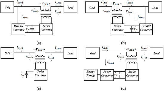
Figure 1.
DVR without energy storage: (a) supply-side-connected shunt converter; (b) load-side-connected shunt converter. DVR with energy storage: (c) variable DC-link voltage; (d) constant DC-link voltage.
According to the obtained equations in [17], the power of the series and the parallel converter is not the same, and the delivered power by the series converter is directly proportional to the voltage sag. Note that maximum loading of current and voltage does not occur simultaneously in the parallel converter because the drawn current is suddenly increasing at severe voltage sag whereas the input voltage decreases. For example, if the source voltage reduces to 0.4 pu in a nominal load, the current of the parallel converter will be 1.5 pu whilst the current of the series converter stays constant at 1 pu. Therefore, the compensation ability for deep voltage sag is diminished by reducing the DC-link voltage to the line voltage value, which is defined as a voltage limitation for compensation.
Load-Side-Connected Shunt Converter
In this topology, the parallel converter and DC-link capacitor are transmitted to the load side in accordance with Figure 1b. The parallel converter from the side of the load provides the required power of the DVR. Hence, the DC-link voltage stays constant due to the feed from the compensated load side.
Due to the supply of the load current and the parallel converter, the current of the series converter increases. The power of the series converter is equal to the power of the parallel converter in the previous setup. The main disadvantage of this setup is that it passes high injecting current through the series converter. For instance, if the source voltage is reduced to 0.4 pu, the series converter current at the nominal load will increase to 2.5 pu, and the parallel converter current will be constant at 1.5 pu. In addition, because of the nonlinear current drawn by the parallel converter from the side of the load, the load-side voltage is polluted to voltage disturbances. The advantage of this setup is the fixed DC-link voltage due to the power supply from the corrected load-side voltage.
2.2.2. Energy Storage-Based Topology
Variable DC-Link Voltage
In this topology, the energy is stored in the DC-link capacitor and in accordance with Figure 1c the parallel converter is removed. At the time of the voltage sag, the DC-link voltage decreases exponentially, and the DVR’s compensation capability is subsequently reduced. Therefore, this topology should be used below the specified voltage level to avoid any problem during compensation.
A series converter or a small auxiliary converter in ordinary conditions can charge the DC-link voltage. In this uncomplicated configuration, when severe voltage sag occurs, a significant amount of stored energy stays useless. This is due to the rapid operation of the converter to inject a high voltage into the network, and it is not an efficient use of storage.
Constant DC-Link Voltage
As shown in Figure 1d, in this setup, separate storage, such as a battery, supercapacitor, and super magnetic energy storage (SMES) with a high power converter is added. The energy through the power converter is transmitted to the DC-link capacitor, and then it is injected into the system. Therefore, the DC-link voltage remains constant during the voltage sag.
Compared to the variable DC-link topology, DVR performance is improved, but due to the addition of separate storage and the power converter, the cost is increased.
2.2.3. Improved Topology of DVR
The overall results of the four discussed topologies show that the variable DC-link voltage has the lowest cost and system complexity (Table 1); it owns the highest score and was selected as the best topology. It also performs poorly in compensating for deep and long voltage sags because of uncontrolled DC-link voltage; but against the disadvantages, it has other salient advantages, such as simple technology and the least overall power rating of DVR converters.

Table 1.
Comparison of the different DVR topologies with the grading: very good (+ +), good (+), poor (-), and very poor (- -).
The load-side-connected shunt converter topology with the privileged features of the ability to compensate long voltage sag, proper DC-link voltage control, and qualified performance in non-symmetrical voltage sags was selected as the second topology. However, this topology has impressive disadvantages, such as the highest overall power rating of DVR converters, inappropriate grid effect, and high cost due to the high power converters. Furthermore, it has the worst impact of power quality on the compensated side of the network as it draws nonlinear currents via a parallel converter during compensation. Accordingly, in spite of the strong emphasis on this topology and lateral suggestions presented by other studies [18,19], it is not suitable for utilization in such a sensitive network due to the reason mentioned above, and other fundamental problems listed in Table 1.
The third rank is related to the constant DC-link voltage topology, which has an excellent function in long and deep voltage sags, preferential DC-link voltage control, acceptable grid effect, and also an admissible overall power rating of converters. By contrast, some disadvantages like its expensive structure, notable size of the energy storage, system complexity, and complicated control have resulted in it coming down in the ranking.
The weakest topology is the supply-side-connected shunt converter. The significant disadvantages of the topology are an uncontrolled DC-link voltage, the unpleasant overall rating of DVR converters, the poor ability to compensate for deep and asymmetric sags, and the tendency of the DVR to draw an asymmetric current from the network in case of asymmetric sag. These remarkable shortcomings cause it to fall to the last order, even though it has a long voltage sag duration capability, the simplicity of control, and an affordable arrangement.
Therefore, according to the analysis conducted, the variable DC-link voltage topology is the most eligible topology for our case, and the ensuing solutions for its drawbacks are presented.
In order to overcome the problem of poor ability of long and deep voltage sag compensation, which is the main cause of dropping the DC-link voltage exponentially at the moment of voltage sag, a battery can be used to stabilize the DC-link voltage.
By placing the battery in this structure (Figure 2), the DC-link voltage controllability will become much better. It should be pointed out that by employing the battery, the required active power for the converter losses is directly supplied and it helps to enhance the stability of the DC-link voltage. The presented solution avoids surplussing the high power converter and its associated problems. Also, by applying a simplified control strategy as described in previous work [6], the complexity of the control in this topology will be resolved.
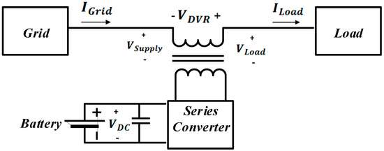
Figure 2.
DVR with optimized constant DC-link voltage topology.
In Table 1, a summary of DVR topologies based on various parameters and scores is presented.
2.3. Dynamic Voltage Restorer Compensation Strategies
By controlling the magnitude and phase angle of the DVR’s injected voltage , the real and reactive power of the DVR can be controlled and implemented using a variety of compensation strategies. The three main compensation strategies are pre-sag, in-phase, and minimum injected active power (energy-optimized). In this section, all compensation strategies and their combinations are considered from various aspects [18,19,20,21,22,23,24].
2.3.1. Pre-Sag Compensation Strategies
By changing the network electrical parameter during sag from to , in the pre-sag strategy, the dropped source voltage is recovered by the magnitude and phase angle prior to the occurrence of voltage disturbance , as shown in Figure 3. In this strategy, in the phase-locked loop (PLL), by locking in the phase angle before the fault, the value of the phase angle is restored to the pre-fault value . This strategy brings the least disturbance to the load side due to maintaining precisely the phase angle of the supply voltage in the pre-fault amount. Thus, this strategy is very appropriate for sensitive loads to the supply-voltage phase angle [20]. As shown in Figure 3, the injected voltage magnitude of the pre-sag strategy is higher than the in-phase strategy. This leads to an injection of high active power and an increase of the required capacity of source storage [21].
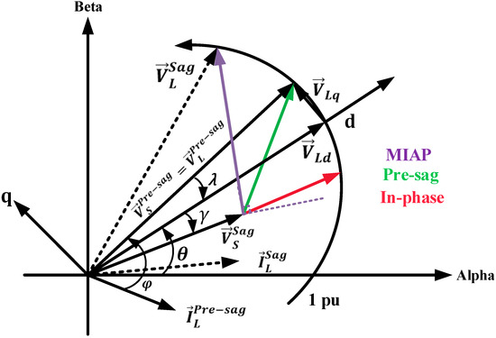
Figure 3.
The diagram of pre-sag, in-phase, and minimum injection active power compensation strategies of the DVR.
2.3.2. In-Phase
In this strategy, DVR’s injected voltage phase angle is similar to grid voltage after the disruption , and unlike other strategies, the magnitude of the injected voltage is minimal (Figure 3). Hence, the need for active power and high-capacity storage is less compared to the previous strategy. Besides, the PLL during compensation is synchronized with the supply voltage during the voltage sag. By changing the load voltage phase during compensation in this strategy, the turbulence and the outage of sensitive loads to the voltage phase occur in the network [22].
2.3.3. Minimum Injection Active Power (MIAP)
In the MIAP strategy, by considering the severity of the voltage sag and limitations on the stored energy of the DVR, it is trying to minimize the delivered active power, and if possible, make it zero. Therefore, the stored energy in the source storage can be used for a longer time. To maximize the injected reactive power and minimize the injected active power, the DVR voltage should be injected perpendicular to the load current, as depicted in Figure 3.
The DVR’s injected voltage in this strategy is absolutely the highest among the other strategies. The amount of MIAP voltage variation depends on the amount of the injected reactive power in which by accurately controlling reference voltages, the amount of the active power delivered by the DVR during the disruption interval will be minimized [24]. The implementation of the MIAP compensation strategy in the d-q coordinate is completely described in detail in [6], and the presented algorithm validates both balanced and unbalanced voltage sag/swell.
2.3.4. Combined Compensation Strategy
In order to exploit the benefits of other strategies and to reduce the existing disadvantages, they can be exploited in combination. In [25], to decrease the DVR voltage magnitude, modulation index, network disturbances, and compensation of large phase jumps, pre-sag and in-phase compensation strategies were combined.
Because of the sensitivity of loads to a sudden phase change, the strategy should be changed quite gradually from the pre-sag to in-phase phases. The starting point of this shift in strategy is when the DC-link voltage or modulation index reaches a threshold limit value. This change in strategy is done by the PLL and injected voltage instead of the pre-sag voltage being synchronized to the grid voltage.
In [26], the pre-sag and MIAP compensation strategies were combined. At first, to reduce the phase jump, DVR operates in pre-sag and then to optimize the stored energy consumption, the compensation strategy changes from pre-sag to MIAP.
The main difficulty of all combined strategies is a long compensation time. So, in this study, due to long and deep voltage sags and other criteria, none of them can be used. The comparison of different DVR compensation strategies for this case study is demonstrated in Table 2.
Table 2.
Comparison of different DVR compensation strategies for this case study with the grading: superior (+ + +), very good (+ +), good (+), poor (-), very poor (- -), and inferior (- - -).
3. STATCOM
Shunt flexible AC transmission system (FACTS) devices, such as STATCOM and static var compensator (SVC), have been extensively used to provide reactive power compensation and support voltage control issues [10]. Since the STATCOM has many benefits, such as a quick response time and better support of voltage instead of other shunt FACTS devices, it was selected for this study [12,27,28]. Moreover, the output reactive power of STATCOM is more than SVC in voltage sag conditions [29]. Additionally, for compensation at this high-level voltage sag, post-fault voltage oscillations of SVC are greater than STATCOM [16]. The control system of STATCOM is the same as the one presented in the previous study [6].
4. Simulation Results and Comparison
In order to verify and validate the performance of the DVR and STATCOM, the TE and ASS were modeled in PSCAD/EMTDC software, as depicted in Figure 4, with the stated parameters in Table 3. The simulation parameters of TE, DVR, and STATCOM are listed in Table 4.
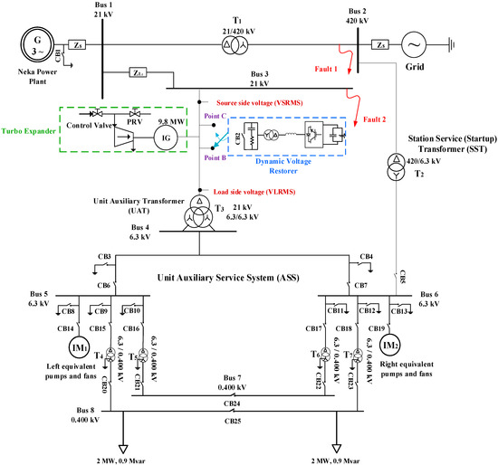
Figure 4.
Schematic diagram of the auxiliary service network (ASS).
Table 3.
Nominal parameters of the Neka power plant network and its ASS.
Table 4.
Nominal simulation parameters of the turbo-expander DVR, and STATCOM.
As the main purpose of this study is to compensate for the SCIG terminal voltage sag under fault conditions, the TE was modeled based on [4], in which the output power of the TE is calculated without using any lookup tables and thermodynamic software. According to the mentioned model, the input mechanical torque of SCIG was simulated; the TE’s generator receives the input torque from the TE via a mechanical shaft.
The scenario design is in line with the most probable events at the power plant. In basic scenarios 1–4, to simulate worst-case disturbances, a temporary fault occurs, with the TE starting concurrently. Furthermore, different types of faults (balanced and unbalanced) and possible locations of the compensators are considered. Scenarios 5–8 discuss the basic scenarios with the DVR compensator located at point B. In addition, in scenarios 9–12 and 13–16, the basic scenarios in the presence of STATCOM compensator at buses 2(420 kV) and 3(21 kV), were also investigated, respectively. It is worth mentioning, the fault occurrence instance and TE start-up for all 16 scenarios was kept the same (t = 0.5 s); it lasts for 1 s.
The four basic scenarios are as follows:
- Scenario 1: Turbo-expander start-up and occurrence of the balanced fault in transmission network (420 kV, 3-phase to ground) simultaneously;
- Scenario 2: Turbo-expander start-up and occurrence of the unbalanced fault in the transmission network (420 kV, 1-phase to ground) simultaneously;
- Scenario 3: Turbo-expander start-up and occurrence of the balanced fault in the ASS (21 kV, 3-phase to ground) simultaneously; and
- Scenario 4: Turbo-expander start-up and occurrence of the unbalanced fault in the ASS (21 kV, 1-phase to ground) simultaneously.
4.1. Dynamic Voltage Restorer Results
Upon the starting of the TE, the generator drawn 63 MVAr of reactive power from the network and makes severe voltage sag in that network [9]. By the presence of the DVR, the reduced supply-side voltage by the TE starting returns to the initial value on the load side voltage (VLRMS), according to Figure 5. All three main compensation strategies considering the amount of injected voltage in the case of the TE starting compensation were simulated. As shown in Figure 6, the amplitude of injected voltage in the MIAP compensation strategy is the largest, the second one is pre-sage, and the last one is in-phase. Therefore, because of the proportionality between the amounts of injected reactive power and the injected voltage magnitude, the MIAP strategy has the highest amount of reactive power injection among other compensation strategies without increasing the size of the DVR’s source storage. Therefore, the MIAP compensation strategy for DVR compensator scenarios (scenarios 5–8) was selected. The simulation results show that in scenario 1, the largest voltage sags of the ASS compared to other basic scenarios (2–4) occur due to a balanced fault in the transmission network. So, as shown in Figure 7a, the source-side voltage (VSRMS) drops to 0.45 pu with 1-s duration.
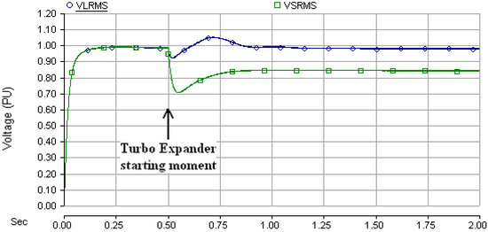
Figure 5.
Supply and compensated load side voltage (VSRMS and VLRMS) in the turbo-expander start-up with the DVR compensator.
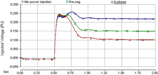
Figure 6.
Comparison of DVR-injected voltage in the minimum power injection, pre-sag, and in-phase compensation strategies.
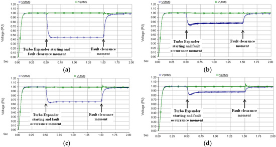
Figure 7.
The DVR performance at point B: (a) Scenario 5; (b) Scenario 6; (c) Scenario 7; and (d) Scenario 8.
In the unbalanced fault scenarios (2 and 4), since the Thevenin impedance in the two scenarios is equal, the higher voltage leads to a higher short circuit capacity (SCC); so, this leads to the voltage drop to 0.72 pu in scenario 2 and 0.81 pu for scenario 4 (Figure 7b,d). Also, in scenario 3, the voltage drop is decreased to 0.37 pu because of the lower voltage level (21 kV) compared to scenario 1 (420 kV).
By placing the DVR at point B (21 kV), all basic scenarios 1–4 were assessed in scenarios 5–8. As shown in Figure 7a, the DVR at point B could rapidly compensate for voltage sag that occurred in scenario 1 and led to voltage drops to 0.45 pu. In other scenarios 6–8, the load side voltage (as shown in Figure 7b–d) in the balanced (scenario 7) and unbalanced fault conditions (scenarios 6 and 8) is clearly compensated for. Figure 7 obviously illustrates the effectiveness of the applied compensation strategy of DVR. Unlike the results of the implemented MIAP compensation strategy in [23], the load side voltage smoothly compensates far better than that of the MIAP strategy. As shown in Figure 7a–d, at the time of both the fault occurring (t = 0.5 s) and thee fault clearing (t = 1.5 s), negligible fluctuations come to pass in the compensated voltage, and there was no voltage sag and swell. In the DVR compensation scenarios (5–8), all voltage sags according to Figure 7a–d, which correspond to 45%, 18%, 27%, and 9%, respectively, in the load side voltage were completely removed.
4.2. Static Synchronous Compensator Results
Different scenarios for determining the best location of compensation were considered. The STATCOM as a shunt FACTS device is connected to bus 3 (21 kV) in scenarios 9–12 and in scenarios 13–16 placed at bus 2 (420 kV). The fault conditions in these eight scenarios are similar to the DVR scenarios. Figure 8 shows the load side voltage (VLRMS) for scenarios 9–12; also, the results of STATCOM in scenarios 13–16 are plotted in Figure 9.
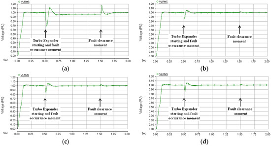
Figure 8.
SATCOM performance at bus 3: (a) Scenario 9; (b) Scenario 10; (c) Scenario 11; and (d) Scenario 12.
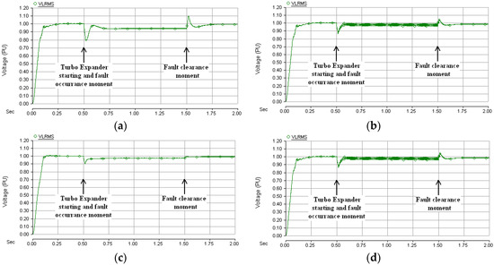
Figure 9.
SATCOM performance at bus 2: (a) Scenario 13; (b) Scenario 14; (c) Scenario 15; and (d) Scenario 16.
In the cases in which STATCOM is installed at bus 3, in scenario 9 (Figure 8a), the most severe voltage sag takes place with a 22% magnitude and 32.5-ms duration. Also, at the fault clearing moment (t = 1.5 s), the voltage swell occurs with a 6.4% amplitude and 18.6-ms duration as well. Scenario 10 (Figure 8b) shows that in the presence of an unbalanced fault at bus 2, the load voltage drops to 0.85 pu (5% voltage sag with 7.3-ms duration).
By changing the fault location in scenarios 11–12 (shown in Figure 8c–d), the voltage sag amplitude in the presence of the balanced and unbalanced fault at bus 3 reaches 8% and 5% for 23.3 ms and 18.6 ms, respectively. Also, no voltage swell conclusively occurs in scenarios 10–12.
To evaluate another possible compensation location, STATCOM was embedded at bus 2 (420 kV). As shown in Figure 9a, the voltage sag increases to 12% for 46.5 ms in the presence of the balanced fault at bus 2. Besides, in the unbalanced fault condition in scenario 14, Figure 9b shows that the compensated voltage falls to 0.86 pu (4% voltage sag with 14.8-ms duration).
As shown in Figure 9c–d, no voltage sag occurs at t = 0.5 in the load side voltage for both fault conditions (balanced and unbalanced), and in the scenarios (13–16), voltage swell never occurs at the fault clearing moment (t = 1.5 s). All in all, the amplitudes and durations of voltage sag and swell are related to the fault voltage level, the type of the fault, and the location and type of the compensator.
4.3. Comparison of Results
The simulation results illustrate that by employing DVR with the MIAP compensation strategy, the voltage sag is instantly compensated. DVR at point B is so well-behaved, which is near the sensitive load. Economically, point B, due to the low voltage level compared to other possible points in high voltage, is more appropriate to reduce DVR costs (especially in terms of the injection transformer).
The STATCOM simulation results in Figure 8 and Figure 9 show that the presence of STATCOM at bus 2 has better performance than bus 3, and by placing STATCOM at bus 3, significant voltage sag occurs. The measurements indicate that the apparent power injected by the DVR is less than that of STATCOM (about 70%). While STATCOM performs compensation for both its downstream and upstream sides, DVR only performs for the downstream side.
In cases of STATCOM compensation, voltage sag and swell eventuated in some scenarios. The utmost voltage sag attributed to scenario 9 on account of balanced fault occurs at bus 3, with a 22% amplitude and 32.5-ms duration; the lowermost is scenario 14, in which the voltage sag magnitude diminishes to 4% with a 14.8-ms extension.
As can be seen in Table 5, where the voltage level is lower, the voltage sag amplitude is decreased; for instance, in scenarios 1 (420 kV) and 3 (21 kV), the voltage sag amplitudes are 45% and 27%, respectively. Since the balanced faults result in a high short circuit current, they have more voltage sag than unbalanced faults, whereas their probability of occurrence is lower than unbalanced types. Considering the locations of the STATCOM shows that by increasing the operating voltage level of STATCOM, close to the severe faults (420 kV), STATCOM has a better performance in compensation. Thus, the best location for STATCOM as the results show is bus 2. As presented in Table 6, due to the passive LC filter, which filters the output of DVR, the amount of harmonic content injected through DVR is less than that of STATCOM. By applying DVR, voltage sag/swell can be removed from the load side voltage waveform in all scenarios, whereas via the action of STATCOM, the voltage sag remains in most scenarios. Overall, regarding the discussed features so far, it is concluded that the most suitable compensator for this issue is DVR at point B.
Table 5.
Comparison of DVR and STATCOM results.
Table 6.
Evaluation of load side voltage frequency spectrum for DVR and STATCOM in scenarios 5 and 13.
4.4. Technical and Economical Evaluation
The application of compensators in the ASS network, besides the compensation of voltage sags caused by TE start-up, input gas MFR fall, and fault conditions for that network, improve the TE performance under fault conditions. Furthermore, local compensation of the reactive power and an increase of the voltage level facilitate the starting conditions for the induction motors (IMs), reduce copper losses and as a result, total ASS consumption decreases. In addition, the reliability of the power plant is enhanced and the voltage of the ASS within the allowed range is supported.
It is worthy to note the voltage fluctuations in the IMs operation, which account for 90% of ASS consumption, and influence their electric parameters, including the efficiency, power factor, and start-up current. Also, it can even change IMs’ active and reactive power demands, which are directly related to the square of the supply voltage.
Hence, by using local compensation, all these issues can be solved. Also, by providing the reactive power required by ASS through the local compensators, instead of using the reactive power produced by the power plant, the capacity of the unit generator is released, and it can be allocated to the more active power generation at full load operation.
The next technical problem in the performance of the TE is the impact of upstream fault which leads to its outage. To provide FRT possibility for TE, the compensator must be installed where the voltage sag is removed from the generator terminal voltage. So, by placing DVR at points B, TE during upstream faults cannot stay operational because it only compensates its downstream side. As the main purpose of this study was to operate the TE and protect the ASS against voltage sag, and because of the inappropriate results of STATCOM in this study and the previous one [6], it is necessary to look for another practicable solution.
Due to the non-repeatability of TE start-up and the lower probability of the inlet gas MFR drop compared to the probability of fault occurrence, regarding the recently performed modifications, the current arrangement does not have technical justification. Hence, after starting TE and reaching steady-state performance, the DVR’s location will be switched to point C. By changing the DVR’s position from point B to C, it can provide FRT capability for TE and support ASS from all aspects.
Providing an economic assessment of the active and reactive power compensated for at the power plant depends on a variety of factors, such as the conditions of the adjacent power plants, the load profile, and how the reactive power is priced.
Based on global prices, DVR costs US$50 per KVAR, so for DVR, with an equivalent capacity of 70 MVAr, the price would be US$3,500,000. The cost of purchasing and installing the TE is assumed to be US$700 per kW. It should be noted that the final guaranteed purchase price of the energy generated by distributed generations is determined based on the price of consumed fuel, the environmental costs, and the price of energy conversion. Accordingly, the proposed guaranteed price with an average of US$0.12 is taken into account for TE generation. Consequently, by the operation of TE with the help of DVR, we have:
There are generally three main methods for evaluating economic projects, such as internal rate of return (IRR), payback method (PM), and NPV. The NPV method is a selecting tool for most financial analysts. The main reasons for selecting NPV are as follows: First, NPV considers the time value of money and future cash flows are expressed based on the value of today’s money; and second, by calculating NPV, a concrete number can be used to compare an initial outlay of cash against the present value of the return. For the economic evaluation of this study, the NPV method as an appropriate and reliable way was used [30].
NPV is determined by calculating the costs (negative cash flows) and benefits (positive cash flows) for each period of an investment. The period is typically one year but could be measured in half-years, quarter-years, or months. After calculating the cash flow for each period, the present value (PV) of each one is obtained by discounting its future value at a periodic rate of return. Finally, NPV is the sum of all discounted future cash flows. A positive NPV results in profit whereas a negative NPV results in the loss.
The NPV is achieved by Equation (5), where t is the time of the cash flows, N is the total number of periods, i is the discount rate, and is the net cash flows for each period (cash inflows minus cash outflows):
In this study, all future cash flows are positive, and the only outflow of cash is the purchase price of the DVR and TE (Equation (4)). The NPV is the PV of future cash flows minus the purchase price. The Neka power plant will cost US$10,360,000 for outgoing cash flow Also, It will provide the equal benefit of US$846,520 for each month, which is obtained by subtracting the cash inflow (US$846,720) from the cash outflow that contains repair and maintenance costs of TE (US$200). The effective annual discount rate is 4% for this project, including the annual inflation rate, interest rate, and risk rate.
As depicted in Figure 10, the NPV value will be positive after 18 months. The NPV’s positivity of this project indicates that the implementation of the project is cost-effective. All costs of the compensator and TE will be paid back within 18 months of TE operation, and then there is a monthly net profit of US$846,520. It is worth mentioning that in the calculation of the payback period, the financial value of the discussed technical benefits of the presence of compensators in the power plant is ignored. By taking into account the mentioned profit and using efficient hybrid designs, such as incorporating the TE with combined heat and power (CHP), the payback period of investment will decrease further from the present value.
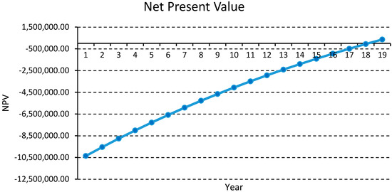
Figure 10.
Net present value diagram.
Finally, a summary of the techno-economic evaluation of this case study is provided in Table 7. The presented table shows a contrast between the two compensators from different features. It shows a significant difference between the score of the DVR and that of STATCOM.
Table 7.
Summary of techno-economic assessment for this case study with the grading: superior (+ + +), very good (+ +), good (+), poor (-), very poor (- -), and inferior (- - -).
By selecting the DVR as the final compensator and executing the presented solution, the possibility of FRT is provided. Also, the achievement of positive NPV proves the project is technically and economically feasible.
5. Conclusions
In this paper, an applicable remedy for supplying ASS o the Neka power plant was provided by utilizing TE during fault conditions. To facilitate the TE operation under the fault conditions, DVR and STATCOM were suggested in series and parallel with the ASS network, respectively. In order to optimize the DVR performance, different types of topologies were investigated and compared in terms of various factors, and improved topologies based on the existing challenges were presented. Also, all basic compensation strategies were reviewed and simulated. The simulation results indicate the effective role of the MIAP compensation strategy and the improved topology of DVR, which in all scenarios could extraordinarily compensate the severe voltage sag. Furthermore, the DVR can respond to disturbances faster with a lower injected harmonic content than the STATCOM.
In this study, by switching the DVR location, all voltage sags caused by the TE starting, the drop in the inlet gas MFR, and the fault occurrence for the ASS network were compensated. Moreover, the possibility of FRT for TE was provided.
The presented analysis confirms the technical and economic feasibility of the project. The economic analysis conducted by the NPV method shows that the project payback time is decreased to 18 months. However, by taking into account the financial value of the technical benefits of the DVR in the ASS, as well as designing high-efficiency hybrid plans, such as integrating TE and CHP, the capital return period will be reduced far less.
Author Contributions
M.N. proposed the main idea, performed the simulations and prepared the original research draft; M.L. supervised the work.
Funding
This research received no external funding.
Conflicts of Interest
The authors declare no conflict of interest.
References
- Daneshi, H.; Khorashadi Zade, H.; Lotfjou Choobari, A. Turbo-expander as a distributed generators. In Proceedings of the IEEE Power and Energy Society General Meeting - Conversion and Delivery of Electrical Energy in the 21st Century, Pittsburgh, PA, USA, 20–24 July 2008; pp. 1–7. [Google Scholar]
- Taleshian Jelodar, M.; Rastegar, H.; Pichan, M. Turbo Expander System Behavior Improvement Using an Adaptive Fuzzy PID Controller. AUT J. Model. Simul. 2017, 49, 23–32. [Google Scholar]
- Babaaei Turkemani, M.; Rastegar, H. Modular modeling of turbo-expander driven generators for power system studies. IEEJ Trans. Electr. Electron. Eng. 2009, 4, 645–653. [Google Scholar] [CrossRef]
- Taleshian, M.; Rastegar, H.; Askarian Abyaneh, H. Modeling and power quality improvement of grid connected induction generators driven by turbo-expanders. Int. J. Energy Eng. 2012, 2, 131–137. [Google Scholar] [CrossRef]
- Norouzi, M.A.; Olamaei, J.; Norouzi, M.J. Improving voltage sag of turbo-expander starting in NEKA power plant by STATCOM. Int. J. Eng. Res. Technol. (IJERT) 2013, 2, 1721–1725. [Google Scholar]
- Norouzi, M.A.; Olamaei, J.; Gharehpetian, G.B. Compensation of voltage sag and flicker during thermal power plant turbo-expander operation by dynamic voltage restorer. Int. Trans. Electr. Energy Syst. 2016, 26, 16–31. [Google Scholar] [CrossRef]
- Shafiul Alam, M.D.; Yousef Abido, M.A. Fault ride-through capability enhancement of voltage source converter-high voltage direct current systems with bridge type fault current limiters. Energies 2017, 10, 1898. [Google Scholar] [CrossRef]
- Liu, S.; Bi, T.; Liu, Y. Theoretical analysis on the short-circuit current of inverter-interfaced renewable energy generators with fault-ride-through capability. Sustainability 2018, 10, 44. [Google Scholar] [CrossRef]
- Yan, L.; Chen, X.; Zhou, X.; Sun, H.; Jiang, L. Perturbation compensation-based non-linear adaptive control of ESS-DVR for the LVRT capability improvement of wind farms. IET Renew. Power Gener. 2018, 12, 1500–1507. [Google Scholar] [CrossRef]
- John Justo, J.; Mwasilu, F.; Jung, J. Doubly-fed induction generator based wind turbines: A comprehensive review of fault ride-through strategies. Renew. Sustain. Energy Rev. 2015, 45, 447–467. [Google Scholar] [CrossRef]
- Hong, L.; Jiang, Q.; Wang, L. A dynamic strategy to improve the ride-through capability of a fixed speed induction generator. Int. Trans. Electr. Energy Syst. 2018, 28. [Google Scholar] [CrossRef]
- Wang, L.; Kerrouche, K.D.E.; Mezouar, A.; Bossche, A.V.D.; Draou, A.; Boumediene, L. Feasibility study of wind farm grid-connected project in algeria under grid fault conditions using D-Facts devices. Appl. Sci. 2018, 8, 2250. [Google Scholar] [CrossRef]
- Yáñez-Campos, S.C.; Cerda-Villafaña, G.; Lozano-Garcia, J.M. Two-Feeder Dynamic Voltage Restorer for Application in Custom Power Parks. Energies 2019, 12, 3248. [Google Scholar] [CrossRef]
- Tien, D.V.; Gono, R.; Leonowicz, Z. A Multifunctional Dynamic Voltage Restorer for Power Quality Improvement. Energies 2018, 11, 1351. [Google Scholar] [CrossRef]
- Farhadi-Kangarlu, M.; Babaei, E.; Blaabjerg, F. A comprehensive review of dynamic voltage restorers. Int. J. Electr. Power Energy Syst. 2017, 92, 136–155. [Google Scholar] [CrossRef]
- Liao, H.; Milanović, J.V. On capability of different FACTS devices to mitigate a range of power quality phenomena. IET Gener. Transm. Distrib. 2017, 11, 1202–1211. [Google Scholar] [CrossRef]
- Godsk Nielsen, J.; Blaabjerg, F. A detailed comparison of system topologies for dynamic voltage restorers. IEEE Trans. Ind. 2005, 41, 1272–1280. [Google Scholar] [CrossRef]
- Jimichi, T.; Fujita, H.; Akagi, H. Design and experimentation of a dynamic voltage restorer capable of significantly reducing an energy-storage element. IEEE Trans. Ind. Appl. 2008, 44, 817–824. [Google Scholar] [CrossRef]
- Jowder, F.A.L. Design and analysis of dynamic voltage restorer for deep voltage sag and harmonic compensation. IET Gener. Transm. Distrib. 2009, 3, 547–560. [Google Scholar] [CrossRef]
- Du, Z.; Chen, Z.; Dai, G.; Yaqoob Javed, M.; Shao, C.; Zhan, H. Influence of DVR on Adjacent Load and Its Compensation Strategy Design Based on Externality Theory. Energies 2019, 12, 3716. [Google Scholar] [CrossRef]
- Nielsen, J.G.; Blaabjerg, F.; Mohan, N. Control strategies for dynamic voltage restorer compensating voltage sags with phase jumps. In Proceedings of the APEC 2001. Sixteenth Annual IEEE Applied Power Electronics Conference and Exposition (Cat. No. 01CH37181), Anaheim, CA, USA, 4–8 March 2001; pp. 1267–1273. [Google Scholar]
- Chung, I.Y.; Won, D.G.; Park, S.Y.; Moon, S.I.; Park, J.K. The DC-link energy control method in dynamic voltage restorer system. Electr. Power Energy Syst. 2003, 25, 525–531. [Google Scholar] [CrossRef]
- Li, G.J.; Zhang, X.P.; Choi, S.H.; Lie, T.T.; Sun, Y.Z. Control strategy for dynamic voltage restorers to achieve minimum power injection without introducing sudden phase shift. IET Gener. Transm. Distrib. 2007, 1, 847–853. [Google Scholar] [CrossRef]
- Mallick, N.; Mukherjee, V. Self-tuned fuzzy-proportional–integral compensated zero/minimum active power algorithm based dynamic voltage restorer. IET Gener. Transm. Distrib. 2018, 12, 2778–2787. [Google Scholar] [CrossRef]
- Meyer, C.; De Doncker, R.W.; Li, Y.W.; Blaabjerg, F. Optimized control strategy for a medium-voltage DVR—Theoretical investigations and experimental results. IEEE Trans. Power Electron. 2008, 23, 2746–2754. [Google Scholar] [CrossRef]
- Rauf, A.M.; Khadkikar, V. An enhanced voltage sag compensation scheme for dynamic voltage restorer. IEEE Trans. Ind. Electron. 2015, 62, 2683–2692. [Google Scholar] [CrossRef]
- Amaris, H.; Alonso, M. Coordinated reactive power management in power networks with wind turbines and FACTS devices. Energy Convers. Manag. 2011, 52, 2575–2586. [Google Scholar] [CrossRef]
- Molinas, M.; Suul, J.A.; Undeland, T. Low voltage ride through of wind farms with cage generators: STATCOM versus SVC. IEEE Trans. Power Electron. 2008, 23, 104–1117. [Google Scholar] [CrossRef]
- Nasiri, M.; Milimonfared, J.; Fathi, S.H. A review of low-voltage ride-through enhancement methods for permanent magnet synchronous generator based wind turbines. Renew. Sustain. Energy Rev. 2015, 47, 399–415. [Google Scholar] [CrossRef]
- Arnold, T. How Net Present Value Is Implemented. In A Pragmatic Guide to Real Options; Palgrave Macmillan: New York, NY, USA, 2014; pp. 1–13. [Google Scholar]


© 2019 by the authors. Licensee MDPI, Basel, Switzerland. This article is an open access article distributed under the terms and conditions of the Creative Commons Attribution (CC BY) license (http://creativecommons.org/licenses/by/4.0/).