Linear Power Flow Method Improved With Numerical Analysis Techniques Applied to a Very Large Network

Abstract

In this paper, we propose a fast linear power flow method using a constant impedance load model to simulate both the entire Low Voltage (LV) and Medium Voltage (MV) networks in a single simulation. Accuracy and efficiency of this linear approach are validated by comparing it with the Newton power flow algorithm and a commercial network design tool Vision on various distribution networks including real network data. Results show that our method can be as accurate as classical Nonlinear Power Flow (NPF) methods using a constant power load model and additionally, it is much faster than NPF computations. In our research, it is shown that voltage problems can be identified more efficiently when MV and LV are integrally evaluated. Moreover, Numerical Analysis (NA) techniques are applied to the Large Linear Power Flow (LLPF) problem with 27 million nonzeros in order to improve the computation time by studying the properties of the linear system. Finally, the original computation times of LLPF problems with real and complex components are reduced by 2.8 times and 5.7 times, respectively.

1. Introduction

Due to the volatility of renewable energy sources (RES), Distribution Network Operators (DNOs) have a great need for faster power flow calculations for simulating different scenarios for network design. DNOs traditionally treat low voltage (LV) and medium voltage (MV) networks as two separate entities where both voltage levels have their own set of assumptions and design policies. However, simulating both the LV and MV networks in a single power flow computation can result in more effective grid management and a new grid design paradigm [1]. On the other hand, this will increase the size and complexity of the power flow problem.

The power flow, or load flow, problem is computed by grid operators to determine whether the power system can function properly for the given generation and consumption. Traditionally, the power flow problem is formulated as a nonlinear system of equations. Therefore, iterative type of methods such as the Gauss-Seidel (G-S), Newton power flow (N-R) and Fast Decoupled Load Flow (FDLF) [2,3,4] are widely used to solve the so-called Nonlinear Power Flow (NPF) problem for transmission networks. However, these conventional power flow methods do not always converge [5] when they are applied to the distribution power flow problem due to some special features of the distribution network, such as radial or weakly meshed structure, high $R/X$ ratio, line’s length and unbalanced loads. Many methods [6,7,8,9] have been developed on distribution power flow analysis and the most of them are based on the Backward-Forward Sweep (BFS) algorithm. Several reviews on distribution power flow solution methods can be found in References [10,11,12].

All iterative power flow solution methods use a direct solver eventually for the linearized NPF problem in every iteration. It has been shown that iterative linear solvers can result in faster performances over sparse direct solvers for very large power flow problems [13,14,15]. In other words, the computational time of NPF computations can be improved by studying the properties of the linear system solved in every iteration and applying Numerical Analysis (NA) techniques such as different reordering schemes, various direct solvers and numerous Krylov subspace methods on them.

Another way to ease the calculation and to speed up the computational time is to linearize NPF equations using some approximations and assumptions in order to obtain the Linear Power Flow (LPF) equations. After the linearization, the resulting LPF equations can be computed only once by direct solvers. Therefore, LPF computations are generally faster than NPF computations and are more suitable to be applied on very large networks with millions of cables for real time simulation. The best-known example of the LPF problem is the DC load flow [16] where linear relations are determined between the active power injections P and the voltage angles $\delta$ and the reactive power injections Q and the deviations of the unknown voltage magnitudes $\Delta \left|V\right|$. Furthermore, the linear power flow formulation is obtained based on a voltage dependent (ZI) load model and some numerical approximations on the imaginary part of the nodal voltages in Reference [17]. Another linear power flow model based on Taylor’s series expansion was proposed in Reference [18]. A direct method taking an advantage of special structure of distribution systems is also developed in Reference [19].

Alternatively, the LPF equations are achieved using only a constant impedance (Z) load model and are used for both strategic studies in Reference [1] and network battery storage control in Reference [20]. This linear model allows for computations to efficiently simulate very large networks, as 22 million buses are simulated in 60 s [1]. However, the linearization quickly loses its accuracy as the voltage drop gets higher and is only to be applied on networks with a ‘relative small’ voltage drop.

In this paper, we propose a fast LPF algorithm improved with NA techniques to solve the Large LPF (LLPF) problem with 27 million nonzeros simulating both the entire LV and MV networks in a single simulation. We investigate the efficiency and accuracy of the LPF computation using a constant impedance (Z) load model by comparing it with the Newton power flow algorithm and a commercial network design tool Vision on various distribution networks. Furthermore, the network of Alliander DNO is used in our linear power flow computations, which contains both the LV and MV power grids and consists of approximately 80,000 km of cable serving over three million customers. The main motivation for using a linear model is that the MV/LV network of Alliander DNO cannot be solved by our NPF solver (Vision). Additionally, MV/LV networks are generally very well conditioned for linear power flow calculations because according to Dutch law and Alliander DNO policies, the voltage drop in the MV/LV network is not allowed to be more than 9% in total. On the LV network, the reactive power and reactance are generally an order lower than the active power and resistance of the network respectively. For this reason, if one simulates the LV grid only and starts from the secondary side of the distribution transformer, it is generally sufficient to only simulate the real part of the network [20]. Therefore, for the application of NA techniques on the LLPF problem, we consider the LLPF problem with first real, and then complex, components.

This paper is structured as follows. Section 2 introduces the mathematical modeling of the LPF problem using a constant impedance load model. In Section 3, the LPF computation is compared with the NPF computation in order to validate the accuracy and efficiency of this linear approach. The case study of the large network of Alliander DNO is given in Section 4. Section 5 describes the application of NA techniques on LLPF problems using real and complex components. Finally, the conclusion is given in Section 6.

2. Linear Power Flow Problem

This section explains how the LPF problem is obtained using a constant impedance load model assuming a balanced network load. The MV and LV network are both modeled using the same physical model. The electricity network can be modeled as a graph $G(\mathcal{N},\mathcal{E})$ where $\mathcal{N}$ represents the network buses and $\mathcal{E}$ the network cables. The relation between the nodal currents $I_{\mathcal{N}}$ and voltages $V_{\mathcal{N}}$ can be defined by Kirchoff’s Current Law:

$$I_{\mathcal{N}}=Y{V}_{\mathcal{N}},$$

(1)

where Y is the so-called nodal admittance matrix. In Equation (1), all variables are given in complex numbers as $V_{\mathcal{N}}=\left|V_{\mathcal{N}}\right|e^{ı\varphi }=V_{\mathcal{N}}^r+ıV_{\mathcal{N}}^m$, $Y=G+ıB$ and $I_{\mathcal{N}}=I_{\mathcal{N}}^r+ıI_{\mathcal{N}}^m$. The admittance matrix can be directly obtained from the network lay-out using the following formula [21]:

$$Y=C{Z}_{\mathcal{E}}^{-1}{C}^{\prime },$$

(2)

where C is a directional connection (branch-node incidence) matrix and $Z_{\mathcal{E}}$ is a square matrix with the corresponding impedance of each cable/edge ($\mathcal{E}$) on its main diagonal.

Generally, the load of the network is modeled as a combination of constant power, constant impedance and constant current (ZIP) [22]. In this paper, we use only a constant impedance load model in order to obtain LPF equations. Furthermore, we model all load buses with nonzero loads (end customers) in the network as constant impedance and connect these buses to the artificial ground buses which are included in the network now as can be seen in Figure 1.

We assume that these additional buses are ground buses and therefore the voltages at these buses are equal to zero or ground voltage level. As a result of this approach, the number of buses in the network increases by the number of load buses with nonzero loads in the network. Theoretically, cables connecting end customers with ground buses have some resistance and reactance. These equivalent resistance $R_{ng}^{\mathrm{eq}}$ and reactance $X_{ng}^{\mathrm{eq}}$ are defined by the following formula:

$$\begin{array}{cc}\hfill R_{ng}^{\mathrm{eq}}& =\frac{V_{\mathrm{ref}}^2{P}_n}{P_n^2+Q_n^2}\hfill \end{array}$$

(3)

$$\begin{array}{cc}\hfill X_{ng}^{\mathrm{eq}}& =\frac{V_{\mathrm{ref}}^2{Q}_n}{P_n^2+Q_n^2}\hfill \end{array}$$

(4)

where $P_n$ and $Q_n$ are active and reactive power consumption of actual load buses with nonzero loads respectively and $V_{\mathrm{ref}}$ is the nominal voltage. Note that Equation (1) cannot be solved directly, because not all elements are known in neither vector $I_{\mathcal{N}}$ and $V_{\mathcal{N}}$. To overcome this problem, we segment the problem in two equations which can be solved separately as:

$$I_{\mathcal{N}}=\left[\begin{array}{c}{I}_1\\ I_2\end{array}\right],Y=\left[\begin{array}{cc}{Y}_{11}& Y_{21}^T\\ Y_{21}& Y_{22}\end{array}\right],V_{\mathcal{N}}=\left[\begin{array}{c}{V}_1\\ V_2\end{array}\right].$$

(5)

We sort the rows of the matrices $I_{\mathcal{N}}$, Y and $V_{\mathcal{N}}$ in such a way that all swing buses and ground buses are placed in $V_1$ and all unknown voltages of remaining buses are placed in $V_2$. In $V_1$, the voltage of the swing buses is set to the nominal level and ground buses are set to ground voltage level. Since the network is modeled as a set of voltage sources and resistances, Kirchoff’s law dictates that $\Sigma I=0$ on every bus in $V_2$. Therefore, $I_2$ is equal to 0 and the power flow equations now become:

$$\left[\begin{array}{c}{I}_1\\ 0\end{array}\right]=\left[\begin{array}{cc}{Y}_{11}& Y_{21}^T\\ Y_{21}& Y_{22}\end{array}\right]\left[\begin{array}{c}{V}_1\\ V_2\end{array}\right].$$

(6)

Since $V_1$ is known, $V_2$ can be solved using the second row of Equation (6) as:

$$\begin{array}{cc}\hfill Y_{22}{V}_2& =-Y_{21}{V}_1,\hfill \end{array}$$

(7)

$$\begin{array}{cc}\hfill Y_{22}{V}_2& =b,\hfill \end{array}$$

(8)

$$\begin{array}{cc}\hfill V_2& =Y_{22}^{-1}b.\hfill \end{array}$$

(9)

Then, we compute $I_1$ as:

$$\begin{array}{c}\hfill I_1=Y_{11}{V}_1+Y_{21}^T{V}_2.\end{array}$$

(10)

Finally, after computing the nodal voltages, the cable currents can be directly calculated by:

$$I_{\mathcal{E}}=Z_{\mathcal{E}}{C}^{\prime }{V}_{\mathcal{N}}.$$

(11)

2.1. Solving in Terms of Only Real Numbers

It is possible to solve the equation in terms of only real numbers in order to ease the calculation or if your software does not support the combination of the complex variables and sparse matrices like the R programming language [1].

2.1.1. Neglecting Imaginary Parts

In LV networks customers use or produce very little reactive power on average. Additionally, due to the fact that the reactive power and reactance are generally an order lower than the active power and resistance, we can neglect the impact of reactive currents, reactive powers and cable reactance. Thus, the equivalent reactance $X_{ng}^{\mathrm{eq}}$ is removed and the equivalent resistance $R_{ng}^{\mathrm{eq}}$ becomes as:

$$R_{ng}^{\mathrm{eq}}=\frac{V_{\mathrm{ref}}^2}{P_n}.$$

(12)

Furthermore, we know that $Y_{22}=G_{22}+ıB_{22}$ and $b=b^r+ıb^m$ in Equation (9). By neglecting all imaginary parts from Equation (9), we obtain the following linear equations as follows:

$$|V_2|=G_{22}^{-1}{b}^r,$$

(13)

where $|V_2|$ is voltage magnitudes, $G_{22}$ is the conductance of admittance matrix $Y_{22}$ and $b^r=-G_{21}\left|V_1\right|$. This makes the power flow computation roughly 50% faster and it might be worth the modeling error introduced by this assumption.

2.1.2. Reformulating Equations with Complex Numbers

Matrix Equation (9) is given as:

$$\begin{array}{cc}\hfill V_2^r+ıV_2^m& ={(G_{22}+ıB_{22})}^{-1}(b^r+ıb^m).\hfill \end{array}$$

(14)

Equation (14) can be reformulated into into the following matrix equation:

$$\begin{array}{cc}\hfill \left[\begin{array}{c}{V}_2^r\\ V_2^m\end{array}\right]& ={\left[\begin{array}{cc}{G}_{22}& -B_{22}\\ B_{22}& G_{22}\end{array}\right]}^{-1}\left[\begin{array}{c}{b}^r\\ b^m\end{array}\right].\hfill \end{array}$$

(15)

After the computation, original $V_2$ is calculated as $V_2=V_2^r+ıV_2^m$ using the computed real $V_2^r$ and imaginary parts $V_2^m$ in Equation (15). In this case, we double the size of the equations but can avoid the complex numbering.

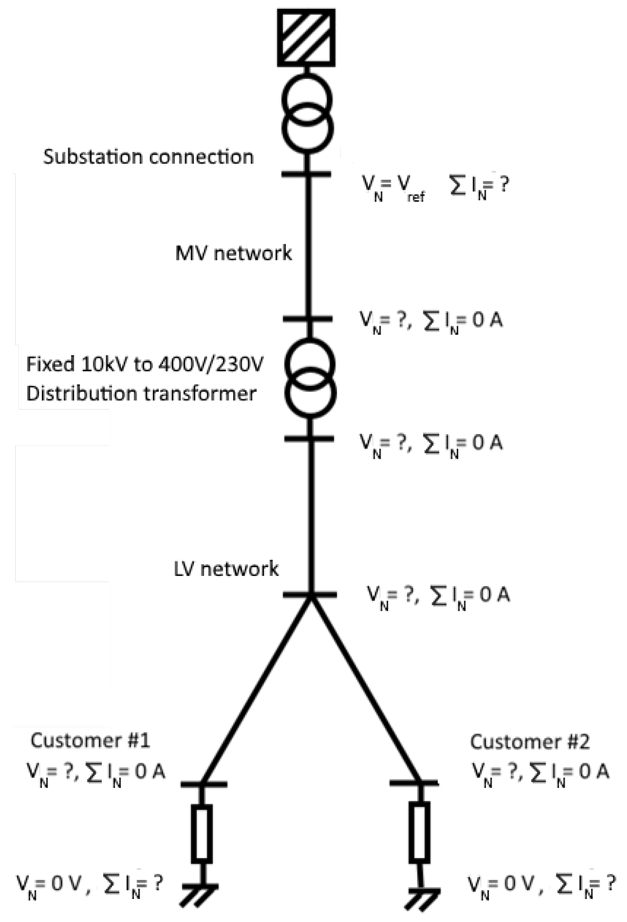
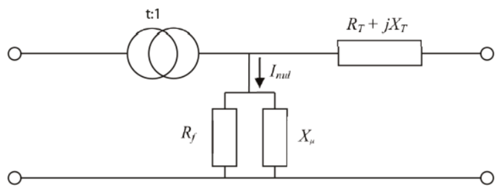
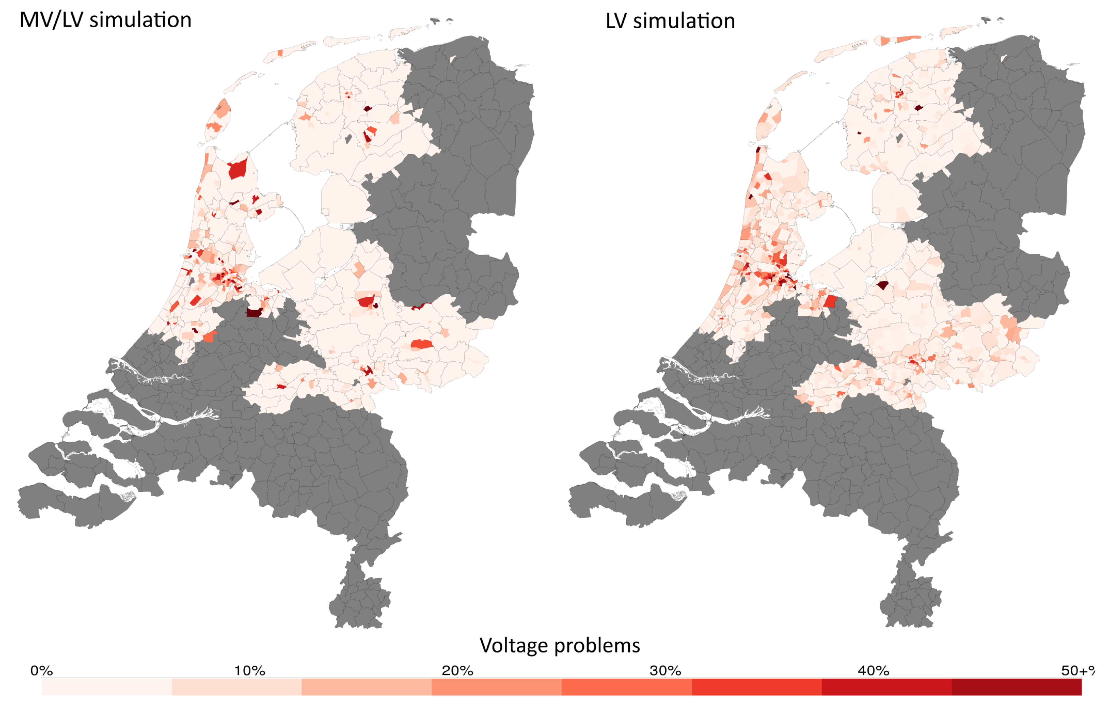
2.2. Modelling MV/LV Transformers

To solve the entire network in a single simulation, the MV/LV transformers are modeled as an RL network [23] as displayed in Figure 2. Transformers are added to the impedance matrix $Z_{\mathcal{E}}$, as the link between the MV and LV network.

In this model, an $\mathcal{E}$ × $\mathcal{E}$ diagonal scale matrix T is defined using the turns ratio t. For every cable behind the secondary side of the transformer, the corresponding value in T is the turns ratio of that transformer. For every cable in the medium voltage network, the corresponding value in the matrix T is 1. The impedance of the link is then scaled using $Z_p=T^2{Z}_s$ where $p,s$ denote the primary and secondary side of the transformer respectively. After the calculation, the turns ratio is used to re-scale the voltage and current to the LV-regime using $V_s=T^{-1}{V}_p$ and $I_s=T{I}_p$.

3. Comparison between Linear and Nonlinear Power Flow Problems

In this section, we compare the LPF approach using a constant impedance load model to the NPF methods using a constant power load model in terms of the accuracy and speed. The Newton power flow method developed in References [24,25] and a commercial network design software Vision [26], are used for NPF computations. Two small balanced distribution networks (Case33 and Case69: network details can be found in Reference [27]) and a large balanced distribution network of Alliander DNO (case991) are considered for the comparison. Network Case991 is the MV network behind the substation Rauwerd, which supplies a significant part of Friesland, a province of The Netherlands. The MV network consists of 991 buses of which 237 are load buses. The network also has significant renewable generation, mostly in the form of wind generators. The same load model is used for the wind generators as for the regular loads, resulting in a negative constant power load in the case of the NPF and a negative constant impedance load in the LPF. The total peak load of this network is 10.3 MVA and the total feed-in peak power is 1.3 MVA. The nominal substation voltage ($V_{\mathrm{ref}}$) is 10.5 kV.

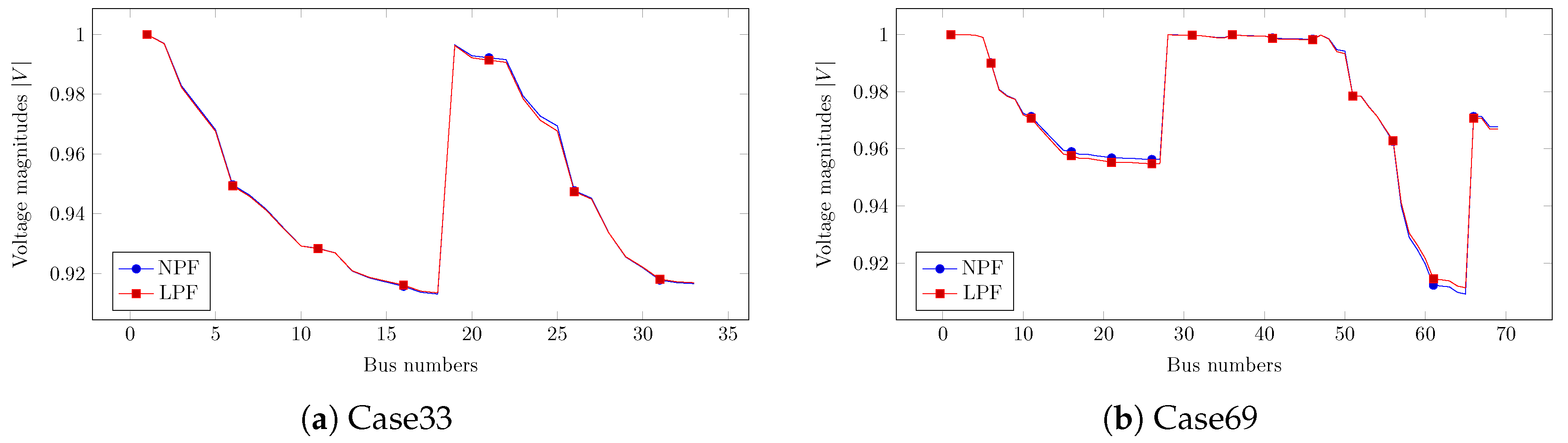
3.1. Comparison to the Newton Power Flow Method

The network currents and voltages have been calculated by applying the LPF and NPF methods on the same network with same properties such as reference voltage and network loads.

Table 1. The CPU time of non-linear power flow (NPF) and linear power flow (LPF) computations (Average of 10 computations) and relative difference.

Test Cases	CPU Time (s)		$\frac{\mathbf{NPF}\left(\mathbf{Time}\right)}{\mathbf{LPF}\left(\mathbf{Time}\right)}$	$\frac{\left|\right|{\mathit{V}}^{\mathit{N}}-{\mathit{V}}^{\mathit{L}}{\left|\right|}_2}{\left|\right|{\mathit{V}}^{\mathit{N}}{\left|\right|}_2}$
	LPF	NPF & Iteration
Case33	0.0005	0.0039 & 3 it	8.3946	$5.87\times {10}^{-4}$
Case69	0.0006	0.0047 & 4 it	8.3585	0.0011
Case991	0.0016	0.0117 & 3 it	7.2025	$7.91\times {10}^{-6}$

shows the total computational (CPU) time of both NPF and LPF computations and relative difference between nodal voltages where $V^N$ and $V^L$ are the computed nodal voltages of NPF and LPF computations respectively. The CPU time also includes data processing time. As shown in the table, the LPF computation is between 7 to 8 times faster than the NPF computation.

In the last column of Table 1, the relative difference $\frac{\left|\right|V^N-V^L{\left|\right|}_2}{\left|\right|V^N{\left|\right|}_2}$ between LPF and NPF solutions, is given and as we can see, the difference is very small. Figure 3 shows the voltage profile of two test cases and compares the results of NPF and LPF computations. The figure visually confirms that the LPF method can be as accurate as the NPF methods.

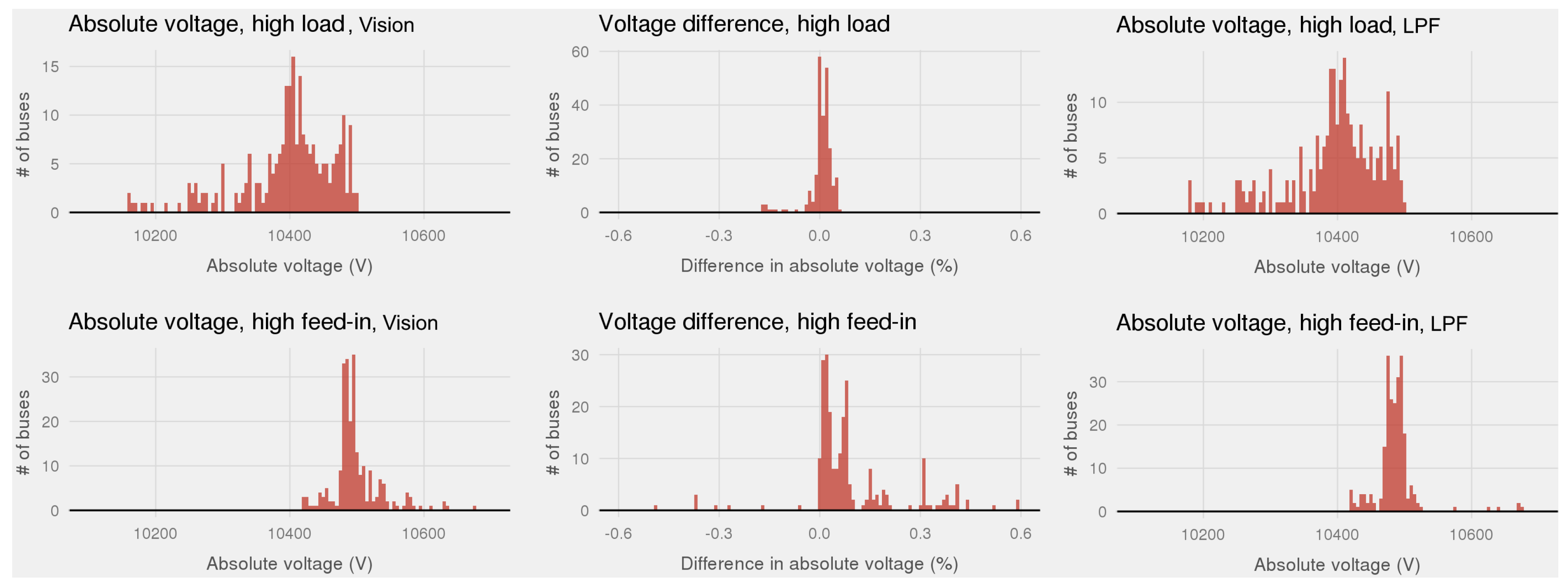
3.2. Comparison to a Commercial Power Flow Software Vision

To further validate the accuracy of the linear modeling approach, the algorithm is compared to a commercial network design tool Vision [26] which is the main software of all Dutch DNOs to dimension their MV networks and uses a constant power load model. The results of the comparison can be found in Figure 4. The figure shows two scenarios; a high load scenario with 100% peak load and 0% feed-in and a high feed-in scenario with 25% peak load and 100% feed-in. The network is relatively heavy loaded because the edge of the network has a voltage drop of around 4%, where 4.5% is the allowed maximum as can be seen in the top-left histogram. It can be observed in right column that the difference between the load assumptions is not more than 0.6%, which is close enough for network design and control purposes.

From both Figure 3 and Figure 4, we can see that the LPF approach using a ‘constant impedance’ load model can be as accurate as classical NPF methods with a ‘constant power’ load model. In addition, the LPF approach is much faster than NPF approach as we have seen in Table 1.

Therefore, this linear power flow approach can be a very powerful tool for electrical grid operators to control the very large networks in real-time.

4. Case Study of Large Dutch Power Grid (LLPF)

In order to demonstrate the impact of integrally simulating the MV/LV grid, a case study has been assembled. The case study focuses on voltage problems. Since the voltage end points are the same for both the MV/LV and LV simulations, the results are easy to compare. The goal of the model is to support large-scale investment policy decisions such as: ‘how many transformers will be overloaded the next 30 years?’ or ‘In which area of the country should more engineers be recruited for cable replacement?’. The model was created for techniques such as time series analysis and agent based modeling which all require evaluating many different load configurations. Several real world MV/LV networks have been studied in literature, some of which have in the order of 100,000 buses [28,29]. However, the networks from these studies are still several orders smaller than the network of this study which has over 24 million buses.

4.1. Data and Assumptions

The network of Alliander DNO is used in our linear power flow computations, which contains both the LV and MV distribution networks and consists of approximately 80,000 km of cable serving over three million customers as shown in Figure 5. It covers over 1/3rd of the total Dutch power grid. The MV network of Alliander DNO consists of 100,000 cable segments whereas the LV network consists of over 24 million buses, three million customers (load nodes), several thousands of generators and around 250 substations. Data sets consist of all cable segments, connectivity and impedance. The connectivity, voltage ratio and impedance of all transformers are used in the power flow computation. The network is mostly radial but some LV networks are strongly meshed and can serve over 100,000 customers.

In line with Alliander DNO policy, a voltage problem is defined as a voltage drop of over 9% in the MV/LV network from the secondary side of the substation transformer to the customer, taking into account that both networks operate on a different voltage level. If only the LV network is considered, the allowed voltage drop is 4.5% from the secondary side of the distribution transformer to the customer. In the MV/LV simulation the nominal voltage ($V_{\mathrm{ref}}$) is assumed to be $10.5$ kV and in the LV simulation the nominal voltage ($V_{\mathrm{ref}}$) is assumed to be 400 V.

Given that the linear model is only valid for relatively low voltage drops, it is important to note that voltage drops of 4.5% on the LV network and over 9% on the MV/LV network are always specified as a ‘voltage problem’ by the DNO. The exact height of the voltage problem is of less importance, as it needs to be solved anyway. The goal of the case study is therefore only to find the problems and not necessarily determining the problem severity.

The current presence of decentralized renewable energy generation is relatively low, around 4% of the total power generation. Generator buses are also modeled as load buses using the constant impedance model. While this is not accurate for the few buses controlling reactive power, it is in line with current Alliander DNO modeling practices.

The network is modeled as a single-phase balanced network, because no data is available of which customer is connected to which phase. While this is a best-case assumption, it is still a good starting point for finding voltage problems in the network and is only an issue for small LV networks with a little number of customers where the law of large numbers does not apply.

To run the linear power flow computation, all three million end users have been given a load of 1.1 kVA with a power factor of 0.95. The power consumption of 1.1 kW is the design peak power for regular households for LV grids containing over forty households. While more detailed data is available within Alliander, it could not be used for publication purposes because of privacy issues. However, the 1.1 kVA assumption yields comparable results on locations with a sufficient number of customers.

4.2. Simulation Results

For this large power flow simulations on LV and MV/LV networks, we use the LPF approach described in Section 2. The LLPF problem with complex components Equation (9) is solved in 58 s on a single processor core using the R programming language. If only active power is considered, the problem is solved in 29 s. All linear algebra is implemented using the Matrix package which is a C wrapper for the Blas and Lapack matrix computation libraries.

The resulting geographical distribution of voltage problems is displayed in Figure 5. Moreover, the absolute number of voltage problems in the MV/LV simulation is 150 thousand, 5% of the total number of customers. The absolute number of voltage problems in the LV simulation is 180 thousand, 6% of the total number of customers. While these percentages are low, they are still very significant as voltage problems can be quite costly to solve.

While the number of voltage problems are in the same order of magnitude between simulations, the locations of the problems are vastly different. The voltage problems overlapped only 20% between the two simulations as can also be observed in Figure 5. The lack of overlap has a severe implication, namely that searching for congestion by only simulating LV networks yields the wrong voltage problem locations. Therefore, it is clear that an identical load configuration will result in a very different layout of voltage problems if the MV/LV network is simulated integrally or only the LV network is taken into account.

It can also be observed from Figure 5 that the problems in the MV/LV simulation are more concentrated compared to the LV simulation due to the fact that a LV network with high loads influences neighboring networks via the MV network. This is very useful information for a DNO, since it also implies that multiple LV voltage problems can be solved by tactically strengthening the MV network.

A subject for future research is a comparison of the calculated problems in this case study with reported problems reported to the DNO. This is not trivial as a good comparison data set is not available. Voltage problems are an emerging issue and currently only very few voltage problems are actually detected by the DNO. This problem is also not easily solved using smart meter data. The smart meter only saves voltage and consumption data from the past 10 days, which is very little information to obtain a good peak consumption pattern. Furthermore, privacy rules and bandwidth limitations also do not allow for constant customer voltage monitoring.

Between the two simulations paradigms (LV only or MV/LV integrally), the integral MV/LV network simulation gives a more accurate estimate of the voltage problem locations as differences in the MV network are taken into account. This conclusion calls for network design using integral MV/LV simulations; a new design paradigm for the DNOs.

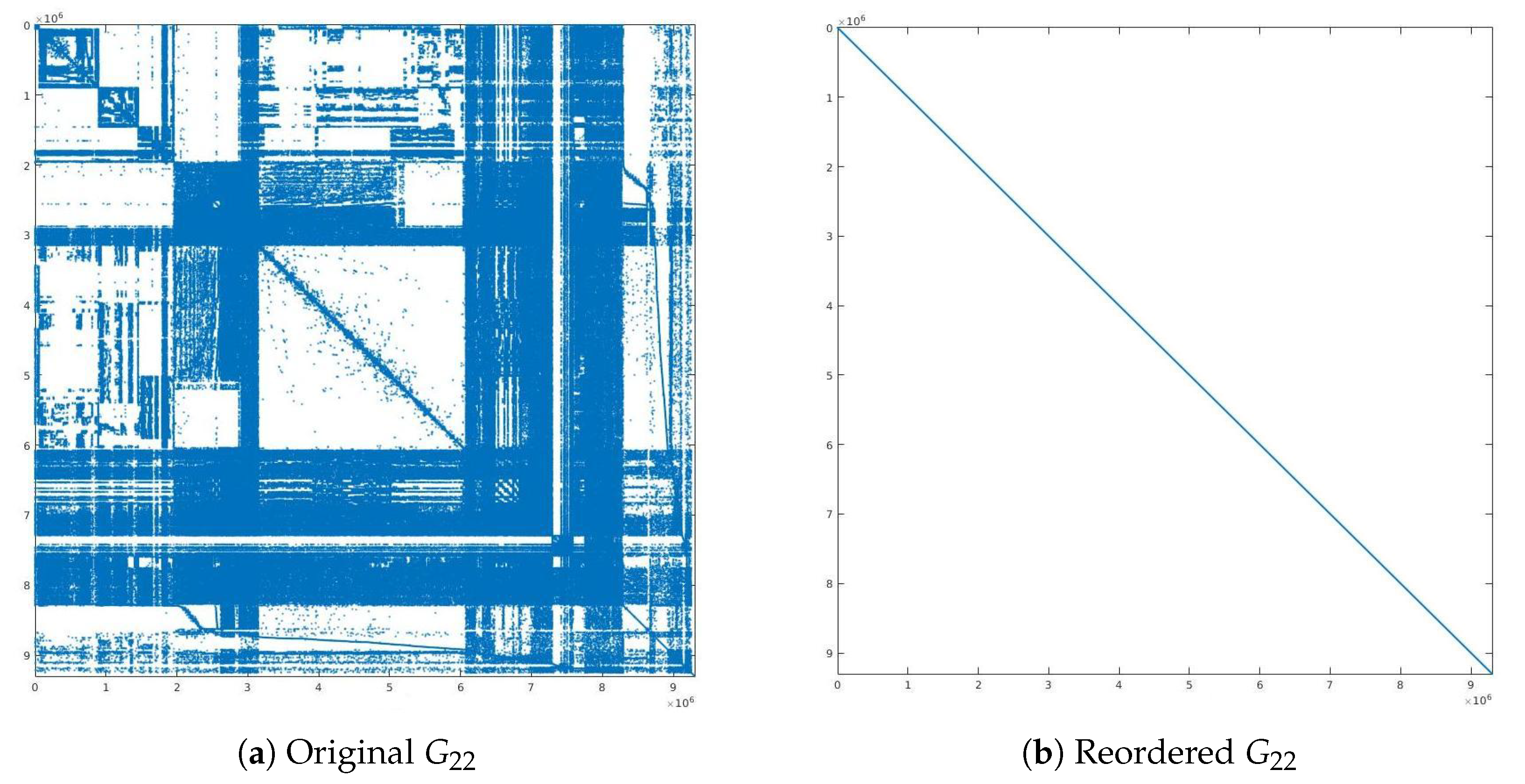
5. Application of Numerical Analysis Techniques on the LLPF Problem

In this section, we show how NA techniques can be used to improve the CPU time of the LLPF computation introduced in Section 4. For this purpose, all solution methods are re-implemented in Matlab. We consider both LLPF problems with complex numbers Equation (9) and without imaginary parts Equation (13). For the numerical experiments, all computations are done on Intel computer i5-6500 3.2 GHz CPU with four cores and 64 GB memory.

5.1. LLPF Problem With Real Components

Let us consider the LLPF problem with real components Equation (13) where the size of matrix $G_{22}$ is $\mathrm{9,300,775}\times \mathrm{9,300,775}$ and the number of nonzeros is $\mathrm{27,867,547}$. Due to the large dimension of the matrix, it is very costly to compute the inverse of the matrix $G_{22}^{-1}$. Therefore, we study the properties of the matrix $G_{22}$ and seek the fastest way to solve Equation (13).

By analyzing matrix $G_{22}$, we observe that $G_{22}$ is a sparse and Symmetric and Positive Definite (SPD) matrix. Due to its SPD properties, we can use NA techniques that are developed for this type of matrices such as the Cholesky decomposition, Incomplete Cholesky (IC) and the Conjugate Gradient (CG) iterative method on $G_{22}$. In addition, some reordering techniques such as Reverse Cuthill-McKee (RCM) and Approximate Minimum Degree (AMD) permutations could improve the properties of $G_{22}$ as well. Figure 6 shows the sparsity structure of $G_{22}$ and reordered $G_{22}$ using RCM.

From the figure, it is clear that the sparseness properties of the matrix $G_{22}$ are improved by using RCM reordering.

For the direct solver, the Cholesky decomposition with RCM reordering could solve the linear system Equation (13) fast. Since $G_{22}$ is a SPD matrix, the best iterative method for matrix Equation (13) is CG. Furthermore, the convergence rate of CG depends on eigenvalues ${\lambda }_k$ of $G_{22}$.

Table 2. The largest and smallest magnitude eigenvalues and the condition numbers for matrix $G_{22}$ and preconditioned $G_{22}$.

Matrix	${\mathit{\lambda }}_{max}$	${\mathit{\lambda }}_{min}$	${\mathit{\kappa }}_2(·)$
$G_{22}$	$9.34\times {10}^8$	$1.38\times {10}^{-3}$	$6.73\times {10}^{12}$
$M^{-1}{G}_{22}$, $L=Chol$	1	1	1
$L=\mathrm{IC}\left({10}^{-5}\right)$	$1.70$	$0.01$	$123.43$
$L=\mathrm{IC}\left({10}^{-6}\right)$	$1.28$	$0.27$	$4.72$
$L=\mathrm{IC}\left({10}^{-7}\right)$	$1.15$	$0.83$	$1.38$
$L=\mathrm{IC}\left({10}^{-8}\right)$	$1.002$	$0.994$	$1.008$

shows the largest ${\lambda }_{max}$ and smallest ${\lambda }_{min}$ magnitude eigenvalues and the condition number ${\kappa }_2(·)=\frac{{\lambda }_{max}}{{\lambda }_{min}}$ of $G_{22}$ and preconditioned $G_{22}$ as $M^{-1}{G}_{22}$.

From the first row of Table 2, we see that the condition number of the matrix $G_{22}$ is very large which means that $G_{22}$ is ill-conditioned. Therefore, using CG without any preconditioner on the linear system Equation (13) cannot improve the computational time since many iterations are required for CG. Thus, the Preconditioned Conjugate Gradient (PCG) method is a proper choice to use instead of CG. In PCG, we solve the transformed system as:

$$M^{-1}{G}_{22}\left|V_2\right|=M^{-1}{b}^r$$

(16)

where M is called a preconditioner and is a SPD matrix. The eigenvalues of $M^{-1}{G}_{22}$ should be clustered around one, resulting in a faster convergence for PCG. Generally, M is obtained as $M=L{L}^{\prime }$ where L is a lower triangular matrix. We can compute L using Cholesky or Incomplete Cholesky decompositions on $G_{22}$ or on reordered $G_{22}$. The eigenvalues of $M^{-1}{G}_{22}$ can be improved by choosing a right preconditioner M for $G_{22}$.

In the second row of Table 2, the Cholesky decomposition is used for L and results in eigenvalues equal to one for the preconditioned $G_{22}$. Therefore, PCG with the Choleksy decomposition is expected to converge after one iteration for Equation (13). However, using the full Cholesky decomposition for L is computationally expensive and the solution time can be larger than using a direct method. In order to decrease the computation time of constructing the lower triangular matrix L, we can use the Incomplete Cholesky decomposition instead of the full Cholesky.

In rows 3–6 of Table 2, we see how the eigenvalues and condition number of $M^{-1}{G}_{22}$ are improved by changing the drop tolerance of IC. Moreover, we can conclude that preconditioner M using IC(${10}^{-8}$) or IC with a drop tolerance smaller than ${10}^{-8}$ for L can be a good preconditioner for matrix $G_{22}$ in terms of the computational time and number of iterations for PCG.

Table 3. Comparison between various numerical analysis (NA) techniques on the large linear power flow (LLPF) problem with real components Equation (13). The best results are given in the bold format.

Algorithms	Time & Iter	$\frac{\left|\right|{\mathit{V}}_2^{\mathit{i}}-{\mathit{V}}_2^{\mathit{d}}{\left|\right|}_2}{\left|\right|{\mathit{V}}_2^{\mathit{d}}{\left|\right|}_2}$	NNZ
$-G_{22}\backslash b^r$	14.32 s	$8.12\times {10}^{-11}$	$\mathrm{27,867,547}$
$G_{22}\backslash b^r$	7.12 s	0
+ RCM	6.94 s	$6.69\times {10}^{-12}$
Cholesky	152.2 s	$7.31\times {10}^{-12}$	$\mathrm{257,293,316}$
+ RCM	5.01 s	$\mathbf{9.51}\times {\mathbf{10}}^{-\mathbf{12}}$	$\mathrm{20,726,961}$
PCG(IC(0)) + RCM	NA	NA	$\mathrm{18,584,161}$
PCG(Cholesky) + RCM	6.24 s & 1 it	$9.51\times {10}^{-12}$	$\mathrm{20,726,961}$
PCG(IC(${10}^{-5}$)) + RCM	6.65 s & 4 it	$0.007$	$\mathrm{19,722,635}$
PCG(IC(${10}^{-8}$)) + RCM	4.96 s & 1 it	$\mathbf{2.42}\times {\mathbf{10}}^{-\mathbf{4}}$	$\mathrm{20,314,280}$

shows the comparison between various linear solvers on Equation (13) in terms of the CPU time, number of iterations and the number of non-zeros (NNZ). All results are averaged over 10 computations. For PCG, the maximum iteration and relative tolerance are set to 100 and ${10}^{-5}$ respectively. The first and second rows of Table 3 are the results of direct solvers using Matlab’s backslash∖operator (R2015a, MathWorks, Natick, MA, USA) without any additional techniques. It is necessary to mention that the CPU time of the first row doubles the CPU time of second row due to the positioning of the minus sign in Equation (7). In addition, if we write the minus sign on the left side of the Equation (7), $-G_{22}$ is not a positive definite matrix which results in large computational time. Therefore, it is better to put the minus sign on the right side of Equation (7) and to keep it inside the vector b.

For the direct solver, the Cholesky decomposition with RCM reordering results in the fastest computational time for matrix Equation (13) as we can see from Table 3. Furthermore, as we expected, IC(${10}^{-8}$) with RCM reordering is the best preconditioner for $G_{22}$ that results in only one iteration in 4.96 s for PCG. However, when IC(${10}^{-8}$) is used for the preconditioner, the relative difference between the direct and iterative solutions $\frac{\left|\right|V_2^i-V_2^d{\left|\right|}_2}{\left|\right|V_2^d{\left|\right|}_2}$ is high compared to other options. Therefore, we also solve the problem Equation (13) with various tolerances for PCG and drop tolerances for IC. Numerical results are given in

Table 4. Numerical results of Preconditioned Conjugate Gradient (PCG) with various tolerances for both Incomplete Cholesky (IC) and PCG.

Time & Iter		Relative Tolerance for PCG
& $\frac{\left|\right|{\mathit{V}}_2^{\mathit{i}}-{\mathit{V}}_2^{\mathit{d}}{\left|\right|}_2}{\left|\right|{\mathit{V}}_2^{\mathit{d}}{\left|\right|}_2}$		${10}^{-7}$	${10}^{-8}$
Drop tolerance for IC	${\mathbf{10}}^{-\mathbf{9}}$	4.96 s & 1 it	4.96 s & 1 it
		& $2.40\times {10}^{-5}$	& $2.40\times {10}^{-5}$
	${\mathbf{10}}^{-\mathbf{10}}$	4.96 s & 1 it	4.96 s & 1 it
		& $2.31\times {10}^{-6}$	& $2.31\times {10}^{-6}$

.

From Table 4, we see that the relative difference $\frac{\left|\right|V_2^i-V_2^d{\left|\right|}_2}{\left|\right|V_2^d{\left|\right|}_2}$ can be improved by decreasing the drop tolerance (${10}^{-9}$, ${10}^{-10}$, ⋯) of IC for the preconditioner $M=L{L}^{\prime }$ while keeping PCG still converge after 1 iteration. Additionally, applying IC gives us smaller NNZ compared to full Cholesky and direct solvers.

Finally, the original computation time (14.32 s) of LLPF problems with real components Equation (13) is improved by 2.8 times (4.96 s) using NA techniques.

5.2. LLPF Problem With Complex Components

In this subsection, we consider the LLPF problem with complex components Equations (9) and (15). For simplicity, let us denote the matrix

$$\left[\begin{array}{cc}{G}_{22}& -B_{22}\\ B_{22}& G_{22}\end{array}\right]$$

in Equation (15) by A. Matrices $Y_{22}$ and A are not positive definite unlike $G_{22}$. Moreover, matrix $Y_{22}$ is symmetric and matrix A is non-symmetric. Therefore, the Cholesky decomposition and CG are not suitable for these types of matrices. Instead, the LU decomposition, Generalized Minimal RESidual (GMRES) and Bi-Conjugate Gradient Stabilized (BiCGSTAB) methods are more convenient to use on matrices $Y_{22}$ and A. For iterative solvers, GMRES and BiCGSTAB, the maximum iteration and relative tolerance are set to 20 and ${10}^{-6}$ respectively.

Table 5. Comparison between numerous NA techniques on the LLPF problem with complex components Equation (9). The best result is highlighted in the bold format.

Algorithms	Time & Iter	$\frac{\left|\right|{\mathit{V}}_2^{\mathit{i}}-{\mathit{V}}_2^{\mathit{d}}{\left|\right|}_2}{\left|\right|{\mathit{V}}_2^{\mathit{d}}{\left|\right|}_2}$	NNZ
Equation (15)	42.6 s	0	$\mathrm{111,470,118}$
Equation (9):   $Y_{22}\backslash b$	17.23 s	$3.03\times {10}^{-11}$	$\mathrm{27,867,547}$
+ RCM	15.58 s	$1.90\times {10}^{-11}$
LU + RCM	7.41 s	$\mathbf{5.84}\times {\mathbf{10}}^{-\mathbf{11}}$	$\mathrm{32,284,123}$
GMRES(ilu(0)) + RCM	177.86 s & 20 it	$0.3427$	$\mathrm{27,867,547}$
BiCGSTAB(ilu(0)) + RCM	56.21 s & 20 it	$0.2503$
GMRES(ilu(${10}^{-8}$)) + RCM	18.75 s & 2 it	$7.23\times {10}^{-8}$	$\mathrm{31,629,906}$
GMRES(ilu(${10}^{-11}$)) + RCM	13.78 s & 1 it	$9.82\times {10}^{-8}$	$\mathrm{32,031,268}$
GMRES(ilu(${10}^{-14}$)) + RCM	14.27 s & 1 it	$9.60\times {10}^{-11}$	$\mathrm{32,244,575}$
BiCGSTAB(ilu(${10}^{-10}$)) + RCM	10.57 s & 0.5 it	$1.12\times {10}^{-6}$	$\mathrm{31,920,611}$
BiCGSTAB(ilu(${10}^{-12}$)) + RCM	10.77 s & 0.5 it	$8.73\times {10}^{-9}$	$\mathrm{32,119,629}$
BiCGSTAB(ilu(${10}^{-14}$)) + RCM	10.92 s & 0.5 it	$9.61\times {10}^{-11}$	$\mathrm{32,244,575}$

shows the comparison between various NA techniques on the LLPF problem Equation (9) in terms of the CPU time, number of iterations and the relative difference between the direct and iterative solutions. In Alliander DNO, Equation (15) is used to solve the LLPF problem because the R programming language does not support complex numbers. Furthermore, from the first and second rows of Table 5, we can see that using Equation (9) to solve the LLPF problem with complex components is almost 2.5 times faster than using Equation (15) when Matlab’s backslash∖operator is used without any additional techniques. Therefore, we use Equation (9) for further experiments.

The same RCM reordering is applied to matrix $Y_{22}$ in order to improve the structure of the matrix. The best computational time (7.41 s) is achieved by the direct solver LU decomposition on the reordered $Y_{22}$ using RCM as can be seen from Table 5. For the iterative methods, the best computation time with the smallest relative difference is obtained by BiCGSTAB with ILU(${10}^{-14}$) as a preconditioner and RCM reordering. However, the best CPU time of the iterative method is still larger than the best CPU time of the direct solver due to the fact that ILU, GMRES and BiCGSTAB are not implemented in the optimal way in Matlab. Furthermore, both LU and ILU decompositions provide relatively similar NNZ for the LLPF problem with complex components.

As a result of the application of NA techniques, the original computation time (42.6 s) of LLPF problems with complex components Equation (9) is improved by 5.7 times (7.41 s).

6. Conclusions

In this paper, we propose a fast LPF method using a constant impedance load model to simulate both the entire LV and MV networks in a single simulation. Mathematical modeling of power systems and transformers is given and the algorithm of the LPF approach is explained in detail. We validate the performance of this LPF approach by comparing it with the Newton power flow method and a commercial network design tool (Vision) on various distribution networks. Our results show that this LPF method can be as accurate as classical NPF methods using a constant power load model and additionally it is much faster than NPF computations. For the largest test network, the entire LV and MV networks of Alliander DNO are used in our linear power flow computations. In our research, it is shown that voltage problems can be identified more efficiently when MV and LV networks are integrally evaluated.

Moreover, NA techniques are applied to the LLPF problem in order to improve the computation time by studying the properties of the linear system. In the numerical analysis, reordering techniques (RCM) and numerous direct solvers (Cholesky, IC, LU and ILU) and various Krylov subspace methods (CG, PCG, GMRES and BiCGSTAB) are chosen and applied to the LLPF problem with both real and complex components. Finally, the original computation times of LLPF problems with real and complex components are reduced by 2.8 times and 5.7 times respectively as a result of the application of NA techniques.

The algorithms in this paper are being applied within Alliander DNO. These applications include: large scale strategic modeling, automatic network design and automatic outage-recovery plans. For the subsequent research, this linear approach will be extended to unbalanced networks and applied to large scale state estimation using thousands of sensors.

References

- Van Westering, W.; Droste, B.; Hellendoorn, H. Combined Medium Voltage and Low Voltage simulation to accurately determine the location of Voltage Problems in large Grids. In Proceedings of the CIRED 27nd International Conference on Electricity Distribution, Madrid, Spain, 3–6 June 2019. [Google Scholar]
- Stevenson, W.D. Elements of Power System Analysis; McGraw-Hill: New York, NY, USA, 1975. [Google Scholar]
- Tinney, W.F.; Hart, C.E. Power flow solution by Newton’s method. IEEE Trans. Power Appar. Syst. 1967, PAS-86, 1449–1460. [Google Scholar] [CrossRef]
- Stott, B.; Alsaç, O. Fast decoupled load flow. IEEE Trans. Power Appar. Syst. 1974, PAS-93, 859–869. [Google Scholar] [CrossRef]
- Tripathy, S.C.; Prasad, G.D.; Malik, O.P.; Hope, G.S. Load-Flow Solutions for Ill-Conditioned Power Systems by a Newton-Like Method. IEEE Trans. Power Appar. Syst. 1982, PAS-101, 3648–3657. [Google Scholar] [CrossRef]
- Cheng, C.S.; Shirmohammadi, D. A three-phase power flow method for real-time distribution system analysis. IEEE Trans. Power Syst. 1995, 10, 671–679. [Google Scholar] [CrossRef]
- Haque, M. A general load flow method for distribution systems. Electr. Power Syst. Res. 2000, 54, 47–54. [Google Scholar] [CrossRef]
- da Costa, V.M.; Martins, N.; Pereira, J.L.R. Developments in the Newton Raphson power flow formulation based on current injections. IEEE Trans. Power Syst. 1999, 14, 1320–1326. [Google Scholar] [CrossRef]
- Chang, G.; Chu, S.; Wang, H. An improved backward/forward sweep load flow algorithm for radial distribution systems. IEEE Trans. Power Syst. 2007, 22, 882–884. [Google Scholar] [CrossRef]
- Martinez, J.A.; Mahseredjian, J. Load flow calculations in distribution systems with distributed resources. A review. In Proceedings of the 2011 IEEE Power and Energy Society General Meeting, Detroit, MI, USA, 24–28 July 2011; pp. 1–8. [Google Scholar]
- Balamurugan, K.; Srinivasan, D. Review of power flow studies on distribution network with distributed generation. In Proceedings of the 2011 IEEE Ninth International Conference on Power Electronics and Drive Systems, Singapore, 5–8 December 2011; pp. 411–417. [Google Scholar]
- Eminoglu, U.; Hocaoglu, M.H. Distribution systems forward/backward sweep-based power flow algorithms: A review and comparison study. Electr. Power Components Syst. 2008, 37, 91–110. [Google Scholar] [CrossRef]
- Zhang, Y.S.; Chiang, H.D. Fast Newton-FGMRES solver for large-scale power flow study. IEEE Trans. Power Syst. 2010, 25, 769–776. [Google Scholar] [CrossRef]
- Idema, R.; Lahaye, D.J.; Vuik, C.; van der Sluis, L. Scalable Newton-Krylov solver for very large power flow problems. IEEE Trans. Power Syst. 2012, 27, 390–396. [Google Scholar] [CrossRef]
- Lahaye, D.; Vuik, K. Globalized Newton–Krylov–Schwarz AC Load Flow Methods for Future Power Systems. In Intelligent Integrated Energy Systems; Springer: Berlin/Heidelberg, Germany, 2019; pp. 79–98. [Google Scholar]
- Schavemaker, P.; van der Sluis, L. Electrical Power System Essentials; Wiley: Hoboken, NJ, USA, 2008. [Google Scholar]
- Martí, J.R.; Ahmadi, H.; Bashualdo, L. Linear power-flow formulation based on a voltage-dependent load model. IEEE Trans. Power Deliv. 2013, 28, 1682–1690. [Google Scholar] [CrossRef]
- Montoya, O.D.; Grisales-Noreña, L.; González-Montoya, D.; Ramos-Paja, C.; Garces, A. Linear power flow formulation for low-voltage DC power grids. Electr. Power Syst. Res. 2018, 163, 375–381. [Google Scholar] [CrossRef]
- Teng, J.H. A direct approach for distribution system load flow solutions. IEEE Trans. Power Deliv. 2003, 18, 882–887. [Google Scholar] [CrossRef]
- van Westering, W.; Hellendoorn, H. Low voltage power grid congestion reduction using a community battery: Design principles, control and experimental validation. Int. J. Electr. Power Energy Syst. 2020, 114, 105349. [Google Scholar] [CrossRef]
- Kirtley, J. 6.061 Introduction to Power Systems Class Notes Chapter 5 Introduction to Load Flow; MIT Open Courseware: Cambridge, MA, USA, 2018. [Google Scholar]
- Kersting, W.H. Distribution System Modeling and Analysis; CRC Press: Boca Raton, FL, USA, 2001. [Google Scholar]
- van Oirsouw, P. Netten Voor Distributie Van Elektriciteit, 2nd ed.; Phase to Phase B.V.: Arnhem, The Netherlands, 2011; Chapter 8. [Google Scholar]
- Sereeter, B.; Vuik, K.; Witteveen, C. Newton Power Flow Methods for Unbalanced Three-Phase Distribution Networks. Energies 2017, 10, 1658. [Google Scholar] [CrossRef]
- Sereeter, B.; Vuik, C.; Witteveen, C. On a comparison of Newton-Raphson solvers for power flow problems. J. Comput. Appl. Math. 2019, 360, 157–169. [Google Scholar] [CrossRef]
- Vision Network Analysis [Application]. Available online: http://www.phasetophase.nl/en_products/vision_network_analysis.html (accessed on 7 December 2016).
- Baran, M.E.; Wu, F.F. Network reconfiguration in distribution systems for loss reduction and load balancing. IEEE Trans. Power Deliv. 1989, 4, 1401–1407. [Google Scholar] [CrossRef]
- Birchfield, A.B.; Xu, T.; Overbye, T.J. Power flow convergence and reactive power planning in the creation of large synthetic grids. IEEE Trans. Power Syst. 2018, 33, 6667–6674. [Google Scholar] [CrossRef]
- Bolgaryn, R.; Scheidler, A.; Braun, M. Combined Planning of Medium and Low Voltage Grids. In Proceedings of the 2019 IEEE Milan PowerTech, Milan, Italy, 23–27 June 2019. [Google Scholar]