Stochastic Optimization of PQ Powers at the Interface between Distribution and Transmission Grids

Abstract

This paper addresses the volt-var control of distribution grids embedding many distributed generators (DGs). Specifically, it focuses on the compliance of powers to specified PQ diagrams at the high voltage/medium voltage (HV/MV) interface while the voltages remain well controlled. This is achieved using a two-stage optimization corresponding to two different classes of actuators. The tap position of capacitor banks is selected on a daily basis, given a stochastic model of the input powers prediction, which allows infrequent actuation and increases the device lifespan. In a second stage, a confidence level optimization problem allows to tune on an hourly basis the parameters of the DGs reactive power affine control laws. Results on a real-size grid show that the combined tuning of these actuators allows the ability to comply with European grid codes while the control effort remains reasonable.

1. Introduction

The variability of active power flows in distribution grids increases with the insertion of distributed generators (DG). As a consequence, the voltages of distribution grids become more fluctuating but can be mitigated by controlling the DGs reactive powers. This leads the DGs, in addition to their active power production, to consume reactive power to compensate over-voltages, which increases the overall consumption of the distribution grid. On the other hand, the growing distance of underground cable generates massive reactive power. Although both problems yield adverse effects, they make the transmission grid voltage control more difficult. In order to reduce power changes at the high voltage/medium voltage (HV/MV) interface, European regulations, specifically the Demand Connection Code (DCC) [1] request that the distribution system operators (DSO) comply with a contractual PQ diagram (Figure 1). Traditionally, capacitor banks (CBs) are used to compensate the reactive power consumption of distribution grids. However, in the context of future grids, their action might not be sufficient, specifically in the cases where the distribution grid produces reactive power, or where a consumption of reactive power stems from voltage control. Therefore, the control of HV/MV interface powers, which have to remain in the contractual diagram, should not rely on CBs alone, but needs to be also supported by the reactive power of some DGs. The optimal coordination of these actuators is the topic of this paper. The main difficulty consists of considering contractual and industrial constraints without undertaking any hardware or grid modification. First, CBs are very fragile and costly devices that should be actuated the least possible, and their lifespan is strongly correlated with the number of tap changes. In this paper, it was chosen that the tap change periodicity should be at most daily. Secondly, today’s communication systems allow, at most, to send information to DGs on an hourly basis and the DG powers are limited by the contractual diagram represented in Figure 2. A reasonable choice is to keep the local droop structure for DG reactive power control and update the parameters to a supervision algorithm. Hence, the supervisory controller of the actuators displays two-time scales, an hourly one for the DGs reactive power controllers, and a daily one for CB control.

A day-ahead rolling window parameter optimization requires us to consider the predictions of power consumption and production. However, by nature, the renewable energies are intermittent and their forecasts are uncertain. A stochastic optimization [2] allows us to encompass the minimization of risks of failure at reasonable actuation prices. In the literature of distribution grid control algorithms, many papers which achieve volt/var stochastic optimization use scenarios or robust optimization in order to take uncertainties into account [3,4,5]. These papers do not require the probability density functions of the input variables; however, they provide little information about the stochastic properties of the voltages and powers inside the grid [6]. Contrary to these procedures, stochastic optimization avoids conservative gain tuning with an unnecessary safety margin, by considering probabilistic density functions and confidence levels as in [7,8,9]. However, these papers address voltage control issues and are not dedicated to HV/MV interface powers control. Few papers deal with the control of powers at the HV/MV interface. The papers [10,11] propose a centralized optimization of DGs local controllers in order to control the powers HV/MV interface but they do not consider capacitor banks. The paper [12] introduces a two-stage optimization of interface powers considering uncertainties. In this paper, the two-time scales are used to schedule the planning and perform the operational optimization, however the limitation of the number of CBs tap change and stochastic objective are not considered. To sum up, these papers focus on control of the HV/MV interface powers without taking advantage of the stochastic nature of the grid variables.

The paper [3] deals with the stochastic nature of the input variables using two time scales, the slow one encompassing capacitor banks and on load tap changer (OLTC) control, and the faster one dealing with reactive power reserves (DG control). However, the objectives and methods are quite different. The paper does not consider an interface PQ diagram. Moreover, the centralized optimization does not keep the industrial local droop-like reactive power control structure. As a result, only a constant reactive power value is supplied for each time interval, which makes it less compliant to disturbances or sparse communication. The optimization methods are based on scenarios instead of probability density functions and confidence levels which makes them efficient but more complex to work out.

Hence, this paper proposes a two-stage stochastic optimization to tune the parameters of the distribution grid HV/MV interface reactive power controllers. The hybrid optimization problem involves both discrete control variables (CBs tap positions), and continuous variables (parameters of DGs reactive power controllers). A model of the grid is proposed, and, under the assumption of truncated Gaussian inputs (production and consumption) powers, voltages and reactive power probability density functions are supplied. In a second time, a voltage control strategy is briefly recalled, which can be based on hourly control parameters updates such as in [9]. Next, the optimal CB tap position is selected using daily forecasts, and the limitations of a strategy using only a constant CB position is explained using PQ diagrams. Then, an optimization program is solved which tunes the parameters of the DG reactive power controllers using hourly forecasts. Finally, the method is applied to a case study.

2. Stochastic Modeling of a Distribution Grid

2.1. Linear Power Flow Models of a Distribution Grid

The commonplace model of distribution grids displays nonlinear equations which make optimization routines very difficult to solve. In order to alleviate this complexity, accurate linear voltage estimations at the steady state were proposed by Bolognani and Zampieri [13,14], assuming a sinusoidal behavior of the voltages and currents which share a common frequency. An extension of this model to a full system [15] considers voltages ($\tilde{\mathbf{V}}$) and powers at the interface (${\tilde{P}}_{HTB}$, ${\tilde{Q}}_{HTB}$) as linear functions of node load/production active ($\tilde{\mathbf{P}}$) and reactive ($\tilde{\mathbf{Q}}$) powers.

$$\begin{array}{ccc}\hfill \tilde{\mathbf{V}}& =& \mathbf{A}\tilde{\mathbf{P}}+\mathbf{B}\tilde{\mathbf{Q}}+\mathrm{𝟙}\widetilde{V_0}\hfill \end{array}$$

(1)

$$\begin{array}{ccc}\hfill {\tilde{P}}_{HTB}& =& {\mathbf{C}}_{\mathbf{P}}\tilde{\mathbf{P}}+{\mathbf{D}}_{\mathbf{P}}\tilde{\mathbf{Q}}+\mathrm{𝟙}{\tilde{P}}_{HTB}^0\hfill \end{array}$$

(2)

$$\begin{array}{ccc}\hfill {\tilde{Q}}_{HTB}& =& {\mathbf{C}}_{\mathbf{Q}}\tilde{\mathbf{P}}+{\mathbf{D}}_{\mathbf{Q}}\tilde{\mathbf{Q}}+\mathrm{𝟙}{\tilde{Q}}_{HTB}^0\hfill \end{array}$$

(3)

where $\mathbf{A},\mathbf{B},{\mathbf{C}}_{\mathbf{P}},{\mathbf{D}}_{\mathbf{P}},{\mathbf{C}}_{\mathbf{Q}},{\mathbf{D}}_{\mathbf{Q}}$ are constant matrices and $\mathrm{𝟙}$ is the vector of all ones. These equations hold under mild assumptions [13,14] that apply to distribution grids as discussed in [15,16], who shows that the accuracy on node voltages remains below 0.001 p.u. and below 0.1 MVA for powers. The values $\widetilde{V_0},{\tilde{Q}}_{HTB}^0$ depend respectively on the OLTC and capacitor banks tap positions. These control variables are supervised by the distribution system operator, while the DGs reactive powers, which are the remaining control variables, are generally equipped with local control laws [17].

The distribution grid used in this paper is displayed in Figure 3. It is a real grid where two distributed generators (3 MW nominal power each) are added without modifying its topology in order to generate overvoltages. The grid has 3441 nodes, 690 loads, 21 generators (mainly PV), which are distributed on 27 feeders, each color in Figure 3 represents a feeder. The maximal consumption of loads is 94.7 MW and 38 MVAr. The nominal power of all generators is 35.5 MW. This network is quite representative of a real distribution grid. The idea is to check whether an appropriate control law allows to add two DGs without topological modifications.

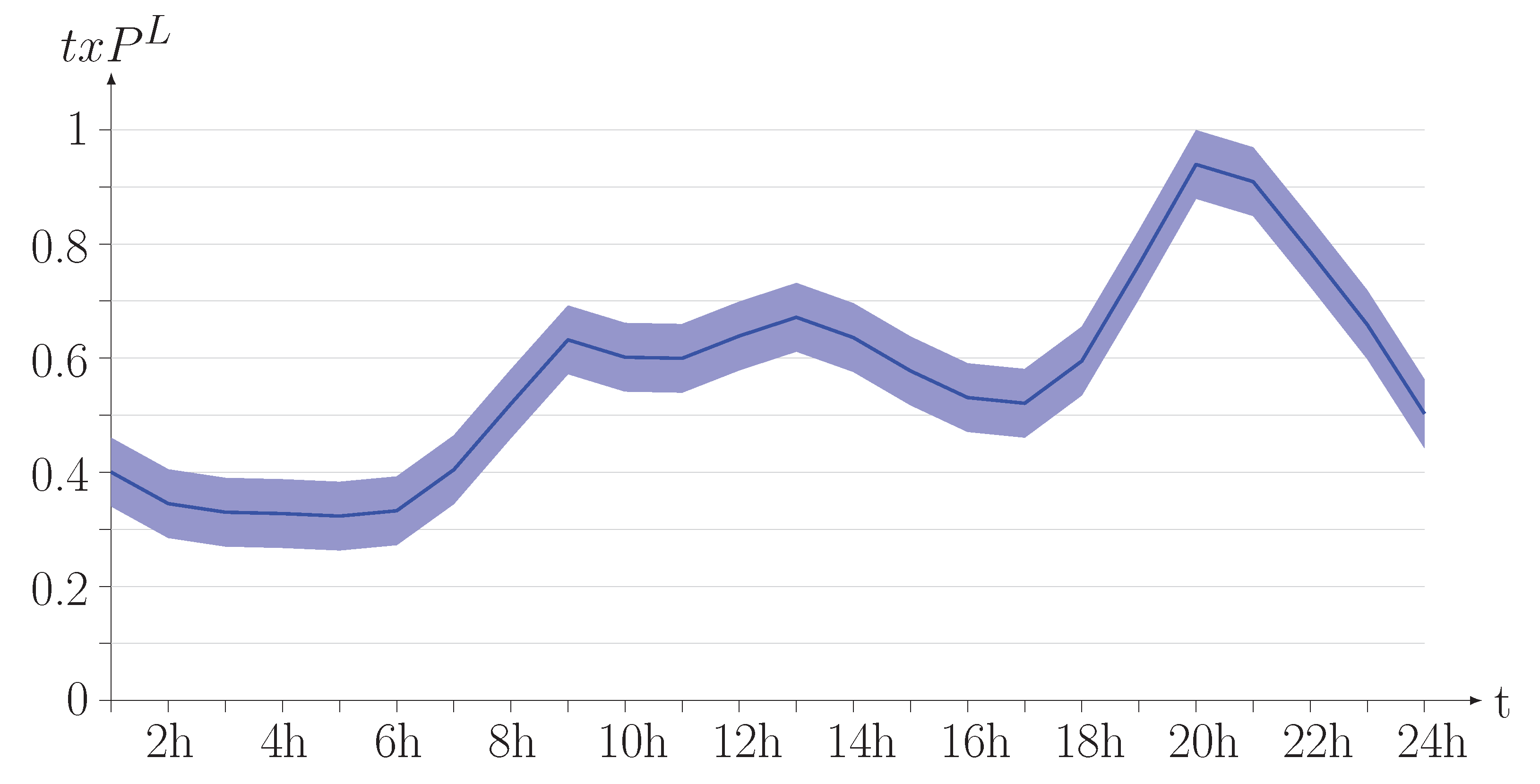
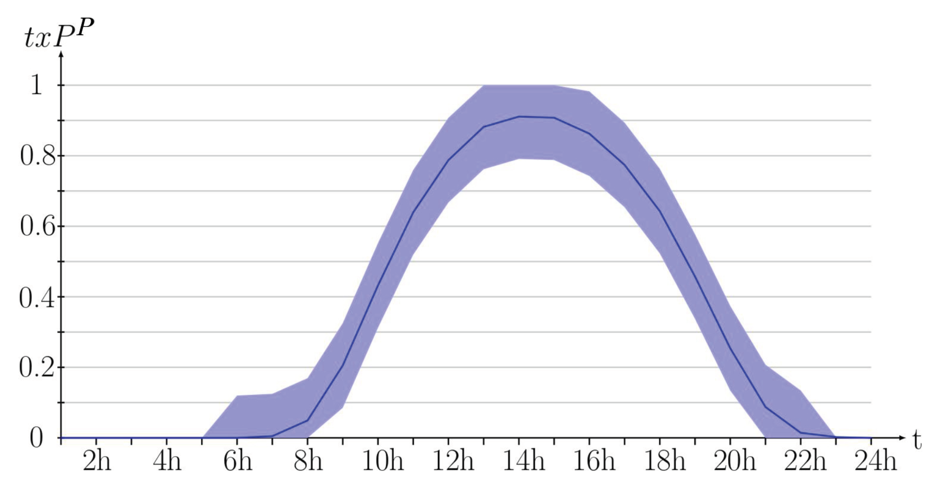
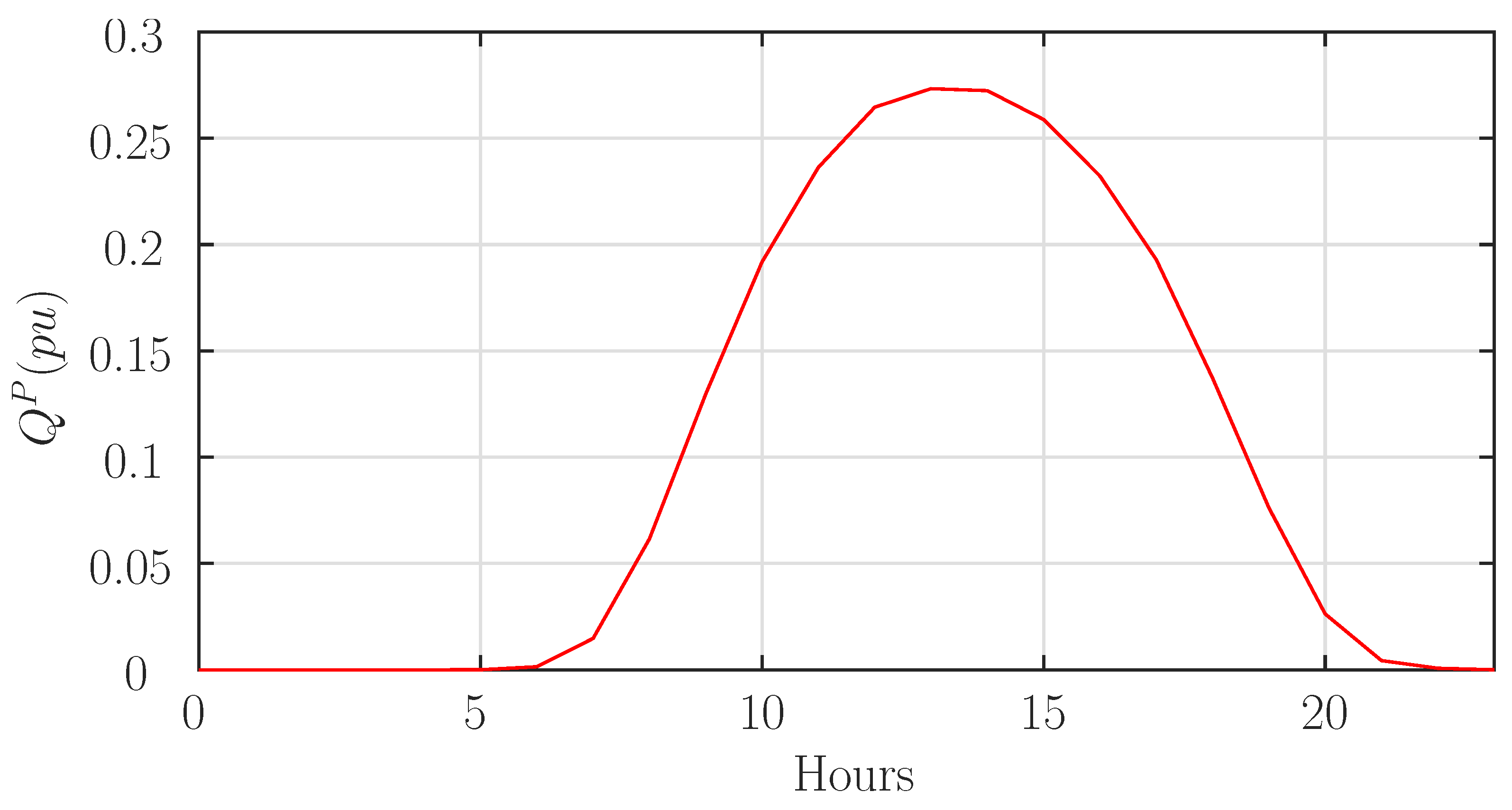
2.2. Daily Stochastic Inputs in a Distribution Grid

The uncontrolled inputs of the network are the consumption and production powers which are very intermittent. Hence, it is important to consider and embed the error estimation of the forecast power into the control algorithm. Indeed, the statistical properties of the node voltages and the HV/MV reactive power can be inferred from the linear model (Equations (1)–(3)) along with forecasting data and model uncertainties. One can obtain not only the voltage expectations, but also their probability density functions and confidence levels.

Future productions and consumption are provided by short term (hourly) most probable forecasts [18,19]. As these forecasts are never accurate, uncertainties inferred from historical data are added (see

Table 1. Uncertainties standard deviations.

Uncertainty (in % of Nominal or Reference Power)	Standard Deviation
Aggregated load forecast uncertainty	3.45%
Load spreading uncertainty	50%
Production forecast uncertainty (photovoltaic energy)	17.16%
OLTC uncertainty	0.005 p.u.

). In the application case, daily consumption and production profiles are illustrated in Figure 4 and Figure 5, they have an hourly basis.

Today, the DSOs usually optimize the parameters of the DGs reactive power controllers over a long horizon. As explained in the introduction, real-time control cannot be implemented in real-life distribution grids, and technological limitations make it preferable to keep traditional droop control structures and update periodically (e.g., hourly) their gains depending on the power inputs. This solution allows us to optimize the interface PQ powers without overloading the communication system. A faster update of parameters can improve the control performance, however it requires a more reliable communication system. However, as the CBs lifespan is strongly correlated to the number of tap changes, it is a reasonable assumption to allow, at most, one tap change to occur on a daily basis. Therefore, the daily profile used for CB control is built from the sum of the hourly forecasts used for DG reactive power control, Figure 6 and Figure 7 display respectively the probability density functions of the consumption and the production during a full day.

These PDFs are represented by Gaussian mixture models over 24 h, combining the hourly Gaussian models proposed in [20]. The consumption consists exactly in a mean of PDFs of Gaussian variables whereas the production is physically bounded between 0% and 100% of its maximal value. In this latter case an important modeling error would be generated if pure Gaussian PDFs were considered. For example, a negative load factor can be remarked in Figure 7. Indeed, the probability density function of a Gaussian variable is supported on the whole real line, and, in some cases, nearly 50% of the density probability lies outside the physical bounds. Hence, the solution consists of using a truncated Gaussian variable instead [9]. Noting ${\mu }_P$ and ${\sigma }_P$ the mean and standard deviation of the forecast power, the corresponding law has three parts:

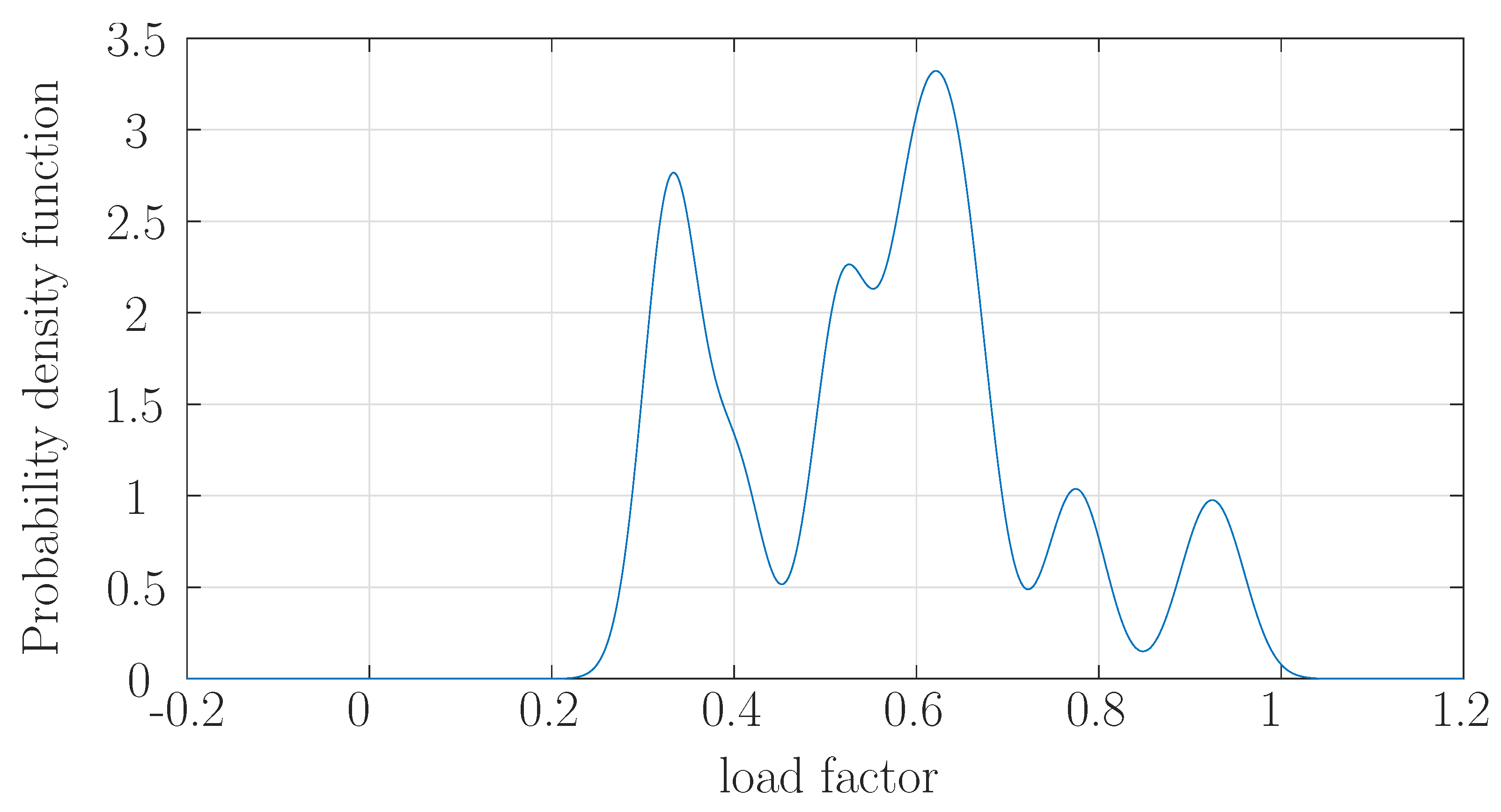
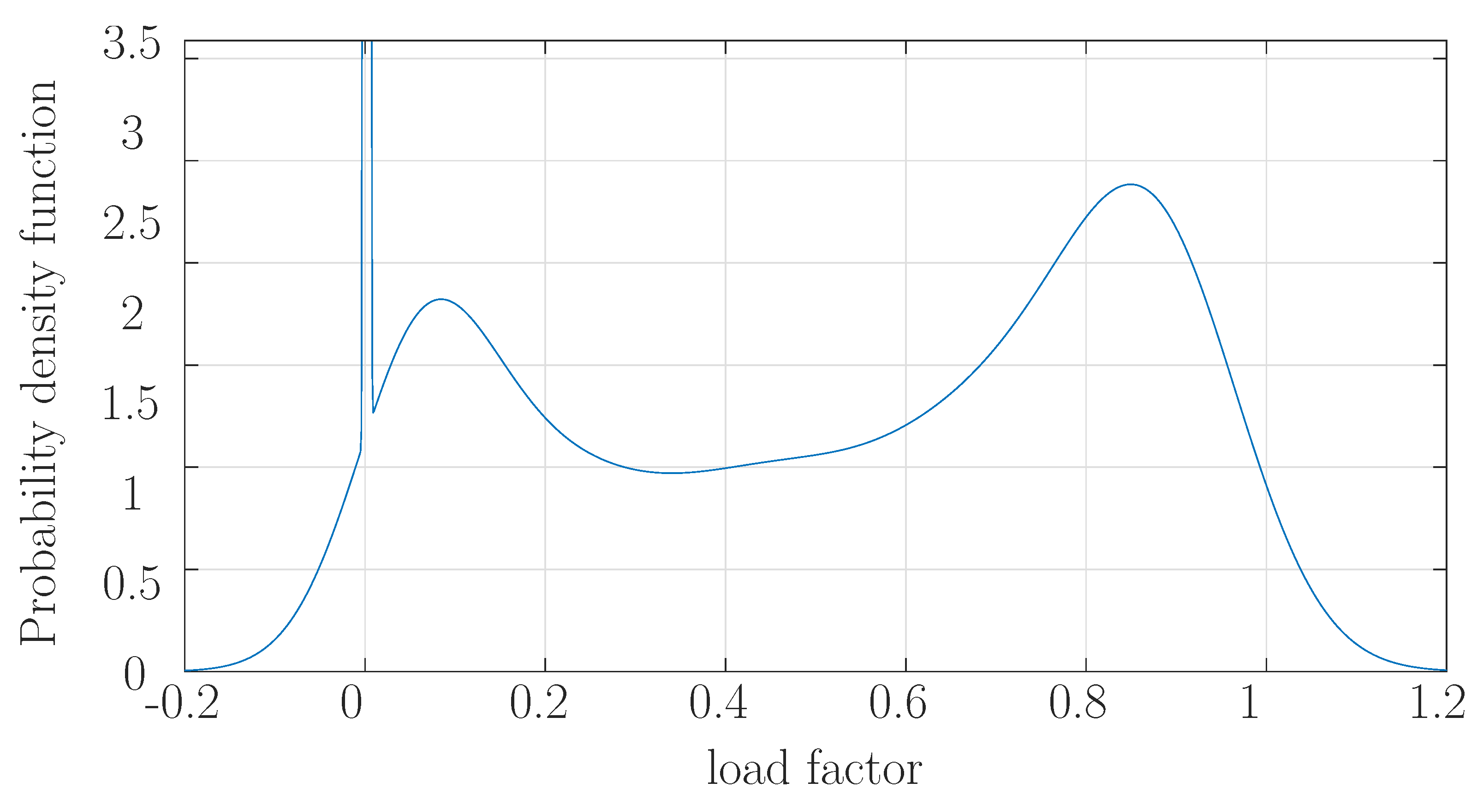
• A truncated Gaussian, with truncations 0 and 1, characteristics ${\mu }_P,{\sigma }_P$:

  $$f_1\left(t\right)=\left\{\begin{array}{ccc}\frac{1}{{\sigma }_P\sqrt{2\pi }}{e}^{-\frac{{(t-{\mu }_P)}^2}{2{\sigma }_P^2}}& \mathrm{if}& 0<t<1\\ 0& \mathrm{else}\end{array}\right..$$

  (4)
• A Dirac distribution at 0 with which area is the probability that the forecast is below 0:

  $$f_2\left(t\right)=\Phi \left(\frac{0-{\mu }_P}{{\sigma }_P}\right)\delta \left(t\right).$$

  (5)
• A Dirac distribution at 0 with which area is the probability that the forecast is above 1:

  $$f_3\left(t\right)=\left(1-\Phi \left(\frac{1-{\mu }_P}{{\sigma }_P}\right)\right)\delta (1-t).$$

  (6)

However, using truncated Gaussian probabilities in a model which will be incorporated into an optimization problem requires a complicated method to propagate truncations over the voltage nodes (for full details, see [9]). A simplified method consists of approximating node voltages by Gaussian variables, which can be achieved if the inputs (production and consumption powers) are themselves Gaussian, since the grid model used in this paper is linear (Equation (1)). It has been chosen to model the input distributions by a Gaussian law obtained with a maximum likelihood approximation. The moments of the distribution are given in Equations (7) and (8).

$$\begin{array}{cccc}\hfill E\left[tx{P}^P\right]=& {\int }_{-\infty }^{\infty }t{f}_1\left(t\right)\hfill & +t{f}_2\left(t\right)\hfill & +t{f}_3\left(t\right)dt\hfill \\ \hfill =& E\left[tx{P}^P\right|0<tx{P}^P<1]\hfill & +0\hfill & +(1-\Phi \left(\frac{1-{\mu }_P}{{\sigma }_P}\right))\hfill \end{array}$$

(7)

$$\begin{array}{cccc}\hfill E\left[{\left(tx{P}^P\right)}^2\right]& ={\int }_{-\infty }^{\infty }{t}^2{f}_1\left(t\right)\hfill & +t^2{f}_2\left(t\right)\hfill & +t^2{f}_3\left(t\right)dt\hfill \\ \hfill & =E\left[{\left(tx{P}^P\right)}^2\right|0<tx{P}^P<1]\hfill & +0\hfill & +(1-\Phi \left(\frac{1-{\mu }_P}{{\sigma }_P}\right))\hfill \end{array}$$

(8)

The mean and standard equation of a Gaussian law truncated in 0 and 1 are found in Equations (9) and (10) where $x\mapsto \varphi \left(x\right)$ is the probability density function and $x\mapsto \Phi \left(x\right)$ the cumulative density function of the standard Gaussian law $\mathcal{N}(0,1)$. Now, these equations can be used to display the node powers as stochastic Gaussian variables. Replacing into the linear model (Equations (1)–(3)) yields in turn Gaussian node voltages, Gaussian active and reactive powers at the transmission–distribution grids interface. The results of this method can be then analyzed hereafter on the studied distribution grid.

$$\begin{array}{ccc}\hfill E\left[tx{P}^P\right|0<tx{P}^P<1]& =& {\mu }_P+{\sigma }_P\frac{\varphi \left(\frac{-{\mu }_P}{{\sigma }_P}\right)-\varphi \left(\frac{1-{\mu }_P}{{\sigma }_P}\right)}{\Phi \left(\frac{1-{\mu }_P}{{\sigma }_P}\right)-\Phi \left(\frac{-{\mu }_P}{{\sigma }_P}\right)}\hfill \end{array}$$

(9)

$$\begin{array}{ccc}\hfill E\left[{\left(tx{P}^P\right)}^2\right|0<tx{P}^P<1]& =& {\sigma }_P^2\left[1+\frac{\frac{-{\mu }_P}{{\sigma }^P}\varphi \left(\frac{-{\mu }_P}{{\sigma }_P}\right)-\frac{1-{\mu }_P}{{\sigma }_P}\varphi \left(\frac{1-{\mu }_P}{{\sigma }_P}\right)}{\Phi \left(\frac{1-{\mu }_P}{{\sigma }_P}\right)-\Phi \left(\frac{-{\mu }_P}{{\sigma }_P}\right)}\right]\hfill \end{array}$$

(10)

3. Two-Stage Optimization Tuning of HV/MV Reactive Power Control

First, it is important to notice that the voltage control inputs have a weak influence on the HV/MV interface reactive power, and, conversely, HV/MV reactive power controllers cause no change of voltage, as long as there is no saturation of the actuators (e.g., when the selected tap number is below the maximum tap). In this case, the actuators used to control the grid voltage are:

• The OLTC which controls the voltage of the secondary node of the distribution transformer. The controller selects the tap which minimizes the difference between the voltage setpoint and the real secondary voltage. Actuation delays are generally added to avoid untimely tap changing and ensure the stability of the electrical system.
• The reactive powers of DGs located in mixed feeder (with both loads and DGs). These DGs are not usually very influential due to their low impact on voltage changes and risks of over-voltage. Their controllers can be either piecewise linear (with a deadband) or linear with the power and the voltage.

The actuators used to control the interface reactive power are:

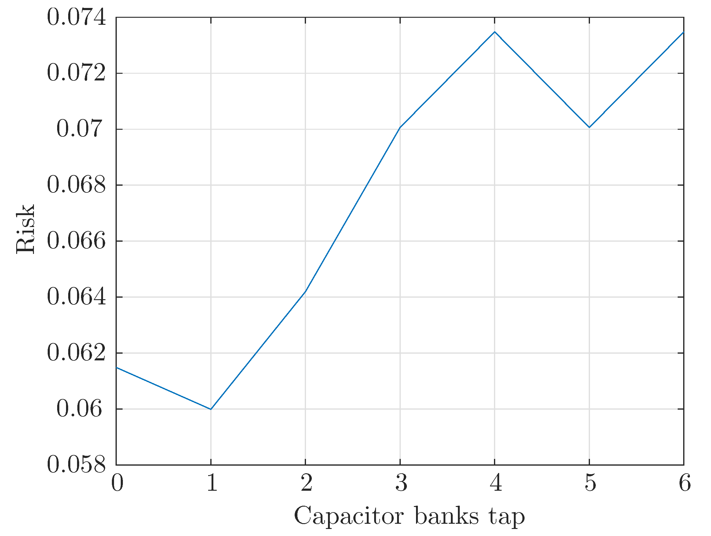
• The capacitor banks which are located at the secondary node of the distribution transformer. Their controller selects a tap for a duration of 24 h.
• The reactive powers of DGs located in dedicated feeders (which embed only DGs). The cables within these feeders are typically sized to avoid overcurrent issues. As a consequence, there are no voltage issues in dedicated feeders. For these DGs, the controllers are affine with the power (it is possible to show that it is useless to use a linear function with the voltage) and can be updated every hour.

Now, the optimization procedure can be achieved independently for each family of actuators (either for voltage or HV/MV reactive power control). This paper proposes a stochastic optimization of the HV/MV interface reactive power considering that the voltage control issue has already been addressed by a classical or advanced algorithm.

3.1. Voltage Control

Voltage control in distribution grids is a widely discussed problem in the literature. This paper is not dedicated to voltage control and any algorithm can be used as long as the parameters remain unchanged during at least one hour.

The European grid code Requirement for Generators [21] defines general guidelines for PQ diagram constraints of distributed generators. These constraints can be customized and adapted to each country. In France, this yields the DG PQ diagram given in Figure 2. This diagram displays reactive power bounds at $-0.35P_i^N$ and $0.4P_i^N$. The value of $tan\left(phi\right)$ = Q/P which minimizes the voltage issues can be inferred directly. Hence, the value $tan\left(phi\right)$ = −0.35 is used for voltage control. In the case where this control law is not able to reach an operating point in the diagram (e.g., $P_i=0.2P_i^N$, $Q_i=0.1P_i^N$), another control law such as an appropriate $Q=f\left(U\right)$ can be used instead [9]. Figure 8 displays the minimum and maximum possible voltages along the 24 hourly windows. In the case study, the node voltages remain between the specified bounds (−0.95; 1.05 p.u.). Designing a sophisticated controller is not necessary to meet the voltage specifications, but the corresponding control effort is important, specifically at daytime with a high production rate, as can be seen in Figure 9.

In order to reduce the reactive power effort, many other control algorithms can be used. As an example, a stochastic optimization based on hourly forecasts has shown nice results and reduced drastically the DGs effort. This method consists in the optimization of the parameters of DGs controllers on a hourly basis using confidence level optimization. The optimization criterion is a weighted sum of confidence levels that node voltages remain within prescribed bounds, of confidence levels that node PQ powers remain within prescribed domains and of the actuation efforts. The DGs controllers can be chosen as linear or piecewise linear. Since the inputs are Gaussian and the power flow model is linear, the model of the node voltages probability density functions are either Gaussian or a sum of truncated Gaussian depending on the DG control structure. The linear case is detailed in [20] and the piecewise linear case in [9].

3.2. Optimization Strategy

After the voltage control is achieved, the HV/MV reactive power control can be carried out. The first step is to select, from daily powers profiles, the CB tap position that maximizes the confidence level that the HV/MV interface remain within the PQ diagram Figure 1. During this tuning procedure, the reactive powers of the DGs of dedicated feeders are not called for. In a second step, DG reactive power control parameters are tuned to further minimize PQ diagram outage using hourly forecast.

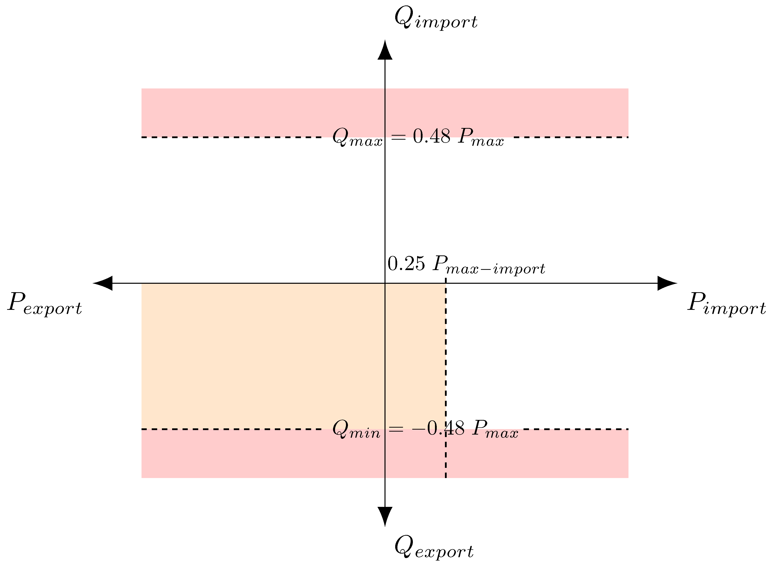
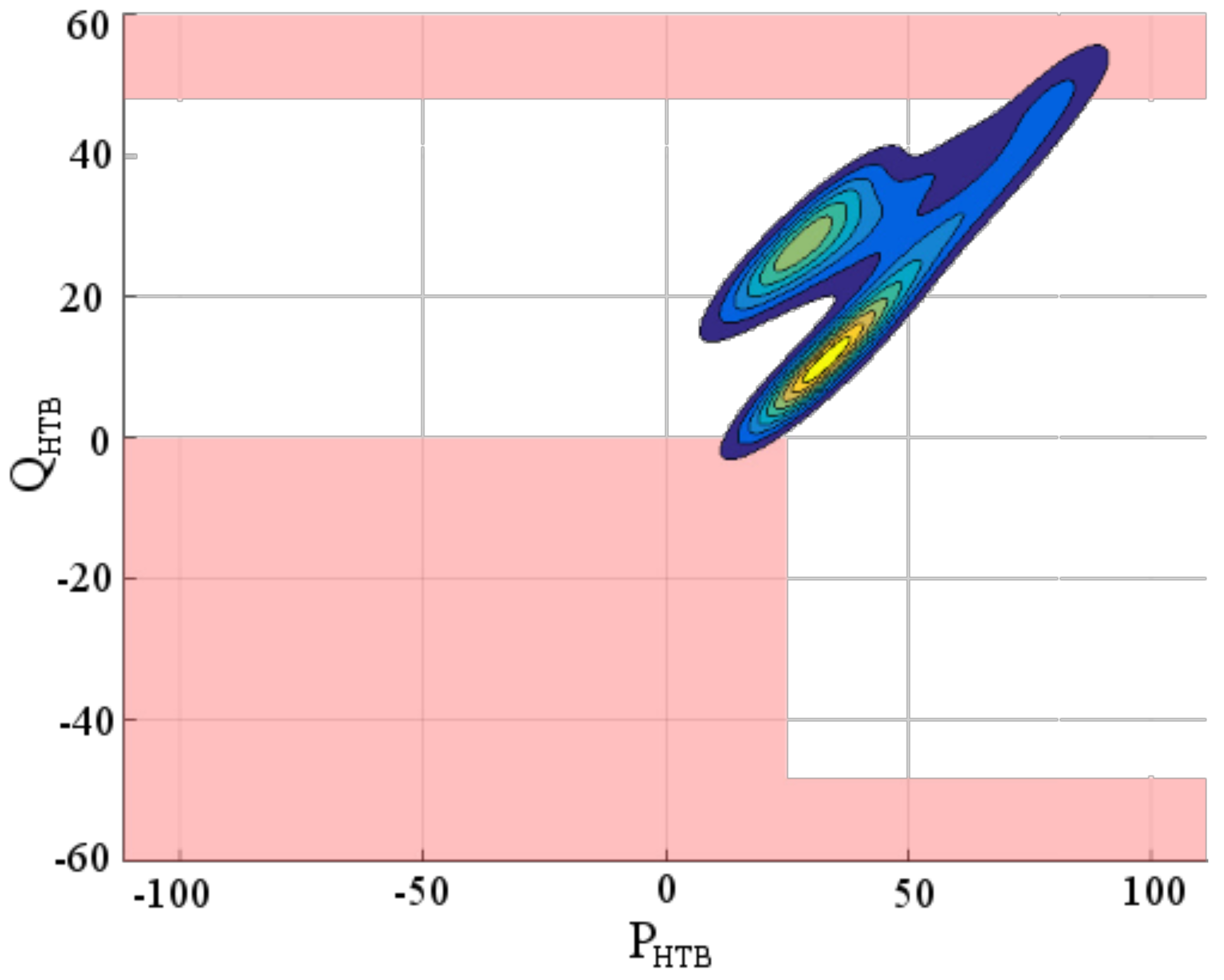
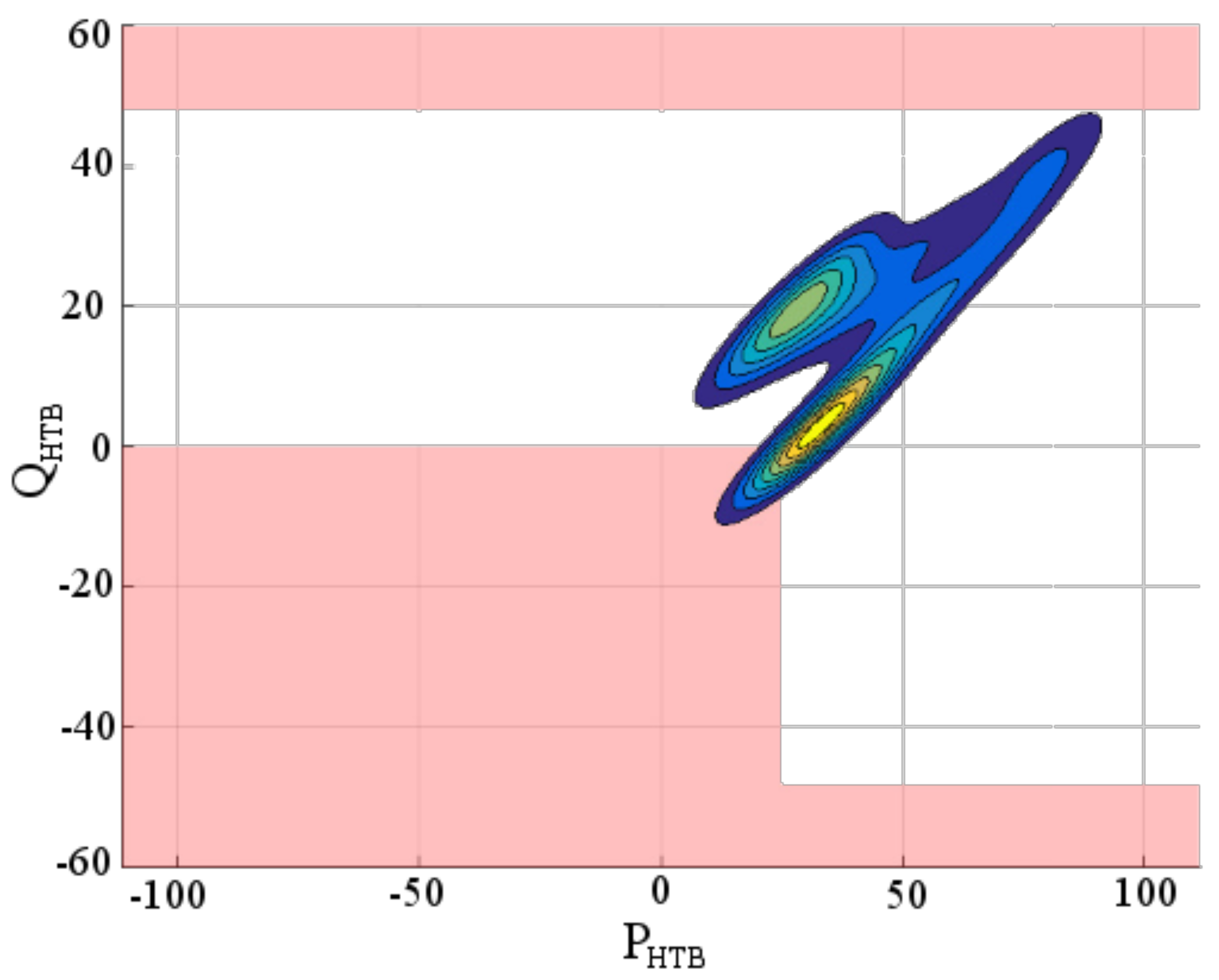
3.3. PQ Diagram Constraints for Fixed Capacitor Bank Tap Position

There are a limited number of CB tap positions, and one can easily consider their daily influence on the PQ diagram at the HV/MV interface. Figure 10 and Figure 11 display the PQ diagram at the interface when the capacitor banks tap position is respectively 0 and 6 (maximum value), which can be compared to the DCC constraints represented in Figure 1.

It is worthy to note that no fixed tap position allows to meet the DCC constraints. When the CBs are idle (position 0), the PQ diagram does not meet the DCC constraints, as the reactive power upper bound is reached. Whenever all CBs are actuated, at the maximum tap position, the stochastic diagram is shifted below, leaving a strong probability for the distribution grid to export reactive power towards the transmission grid.

As the number of tap positions (the discrete optimization variable) is small, finding the optimal tap can be achieved easily by computing the confidence level of the DCC diagram violation for each position, as displayed in Figure 12 and comparing the different values. The optimal tap position is the tap 1, which yields PQ specifications violation risks to 6%. This is above the requested maximum level which is 5%. Hence, it is necessary to coordinate CB tap control with DGs reactive power controllers.

A fine look at the time profiles allows to analyze the source of PQ diagram specifications violations and set the DGs activation periods which correspond to different configurations:

• The consumption exceeds 48% of the maximal power ( time windows 20 h and 21 h). The DG droop controllers may inject reactive power to decrease the reactive power consumption in the grid.
• On the contrary, when the consumption is quite low ($P_{HTB}<0.25\times P_{max}$), reactive power can be exported to the transmission grid (hourly windows 3, 4, 5 and 6 h). On the contrary, DGs can be requested to compensate the phenomenon by consuming reactive power.

This subsection shows how to perform the first stage of the optimization routine, that is to select the CB tap position that minimizes PQ diagram outage at the HV/MV interface. Once this tap is selected, the second stage consists in tuning the DG reactive power control parameters using confidence level optimization.

3.4. Setting a Confidence Level Optimization Problem to Tune DGs Reactive Power Controllers Parameters

In this second stage, the DGs reactive power controllers parameters are updated hourly to minimize the risk of outage of the specified HV/MV interface PQ diagram. The objective of this optimization is to tune the parameters of each DG. It is recalled that the DG local control laws are affine: $Q_i^p={\beta }_i{P}_i^p+Q_i^0$.

This stochastic optimization program considers sub-objectives which involve means, variances and confidence levels:

• Maximize confidence levels ${\lambda }_i$ such that the DG power at node i remains within the contractual PQ domain;
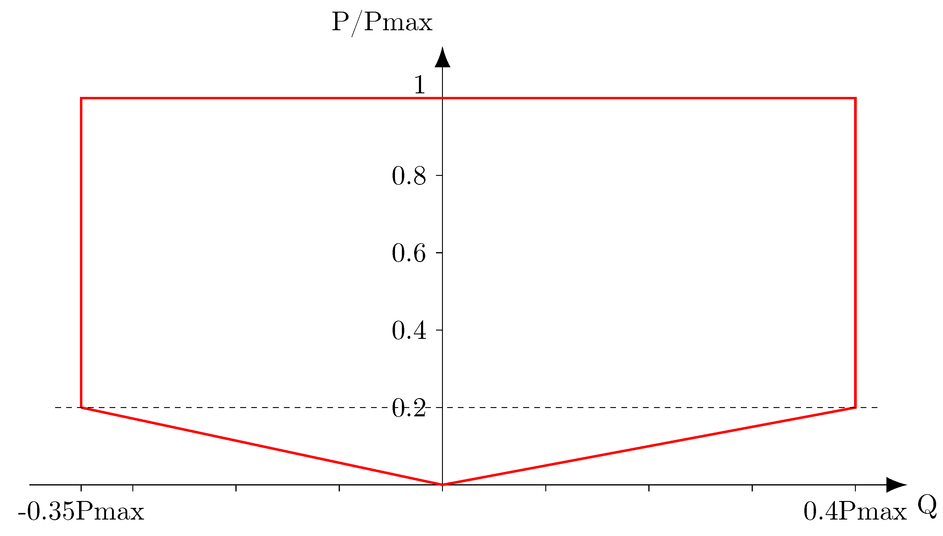
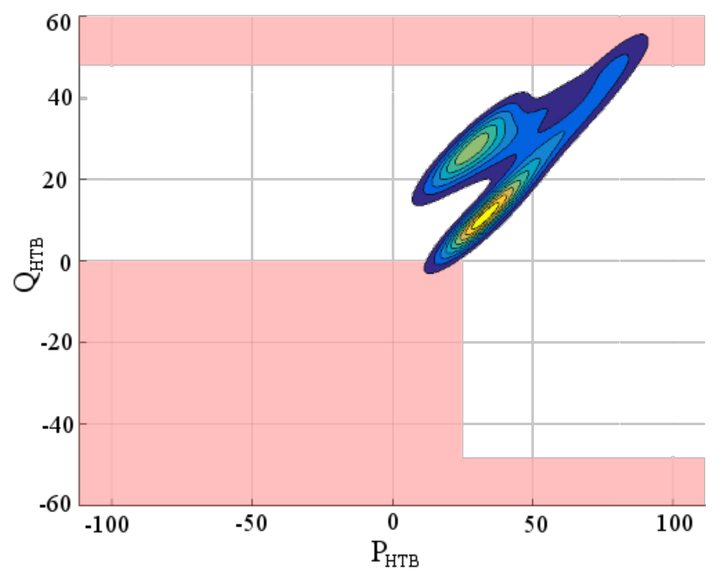
• Maximize confidence level $\nu$ such that the powers at the HV/MV interface $({\tilde{P}}_{HTB},{\tilde{Q}}_{HTB})$ remain within the PQ diagram specified in the grid codes, see Figure 1.
• Minimize DG efforts $E\left[\right|\frac{{\tilde{Q}}_i^p}{P_i^N}\left|\right]$.
• Minimize the variance of the reactive power at the HV/MV interface $var\left(Q_{HTB}\right)$.

The global objective is a weighted sum of these sub-objectives: Equation (11).

$$\underset{x_{\beta },x_Q}{\max }\underset{i=0}{\overset{n}{min}}{\omega }_1{\lambda }_i+{\omega }_2\nu -\sum _{i=0}^n\left(\frac{{\omega }_3}{m}E\left[\right|\frac{{\tilde{Q}}_i^p}{P_i^N}\left|\right]\right)-{\omega }_{4}var\left(Q_{HTB}\right)$$

(11)

The optimization program embeds additional specific constraints described hereafter:

• Confidence levels ${\lambda }_i$ should be above a specified minimal value ${\lambda }_s$ for all nodes.
• Confidence levels ${\delta }_l$ should be above a specified minimal value ${\delta }_s$ for all nodes (that is the confidence levels that the line currents are lower than the maximum authorized current). This constraint is always verified in this study, whatever the consumption or production rates.
• Confidence level $\nu$ should be above a specified minimal value ${\nu }_s$.

The set of constraints is summarized in Equations (12)–(14).

$$\begin{array}{cc}\hfill {\lambda }_i& >{\lambda }_s\forall GEDs\hfill \end{array}$$

(12)

$$\begin{array}{cc}\hfill {\delta }_l& >{\delta }_s\forall conducteurs\hfill \end{array}$$

(13)

$$\begin{array}{cc}\hfill {\nu }_i& >{\nu }_s\forall GEDs\hfill \end{array}$$

(14)

In this study, the values ${\lambda }_s={\delta }_s={\nu }_s=0.95$ are considered. The selection of the weighting factors is done using a Pareto front study in the same way as [9], leading to the following numerical values in Equations (15)–(18).

$$\begin{array}{cc}\hfill {\omega }_1& =0.9995;\hfill \end{array}$$

(15)

$$\begin{array}{cc}\hfill {\omega }_2& =0.9995;\hfill \end{array}$$

(16)

$$\begin{array}{cc}\hfill {\omega }_3& =0.0005\hfill \end{array}$$

(17)

$$\begin{array}{cc}\hfill {\omega }_4& =1;\hfill \end{array}$$

(18)

The previous optimization problem is applied to the case study. The DG effort contribution is restricted by the producers PQ capability diagram. When the production is above 20%, the reactive power is bounded within [−0.35; 0.4] p.u., the limitations shown in Figure 2 are even more severe when the production is weaker.

Similar to the stochastic optimization of the voltage control addressed in [20], this problem is convex and can be solved using a classical interior point method (Matlab routine).

Table 2. DG optimized parameters.

Hour	${\mathbf{txP}}^{\mathit{P}}$	${\mathit{\beta }}_{\mathit{i}}$	${\mathit{Q}}_{\mathit{i}}^0$	PQ Diagram Outage Risk	PQ Diagram Outage Risk
				${\mathit{Q}}_{\mathit{i}}^0$ et ${\mathit{P}}_{\mathbf{cond}}=1$	Optimized Parameters
1	0	0	0	0.0011	0.0011
2	0	0	0	0.0038	0.0038
3	0	0	0	0.0050	0.0050
4	0	0	0	0.0052	0.0052
5	0	0	0	0.0056	0.0056
6	0.0000	0	0	0.0048	0.0048
7	0.0048	0	0	0.0010	0.0010
8	0.0492	0	0	0.0000	0.0000
9	0.2053	0	0	0.0000	0.0000
10	0.4323	0	0	0.0000	0.0000
11	0.6394	0	0	0.0000	0.0000
12	0.7876	0	0	0.0000	0.0000
13	0.8818	0	0	0.0001	0.0001
14	0.9109	0	0	0.0000	0.0000
15	0.9078	0	0	0.0000	0.0000
16	0.8626	0	0	0.0000	0.0000
17	0.7739	0	0	0.0000	0.0000
18	0.6430	0	0	0.0000	0.0000
19	0.4573	0	0	0.0009	0.0009
20	0.2540	0	0.235	0.0185	0.0072
21	0.0875	2	0	0.0126	0.0107
22	0.0144	0	0	0.0012	0.0012
23	0.0024	0	0	0.0000	0.0000
24	0	0	0	0.0001	0.0001
Cumulative risk				0.0600	0.0467

displays the optimized droop gains and constant terms and the corresponding DCC diagram outage risk when reactive powers are zero. In order to balance control efforts, these should be identical for all DGs. In this table, it can be seen that DGs reactive power controllers are not activated except for the time windows 20 h and 21 h. For both times, the initial outage risks are higher than 1%, which greatly contributes to the overall risk. Hence, the optimization routine should pay a special attention to decrease the outage risks in these time windows. At time 20 h, a constant reactive power demand $Q_i^0=0.235$ reduces the risk from 0.0185 to 0.0072. At time 21 h, the active power is low (lower than 0.2 pu) and a maximum droop gain value is selected.

On a daily basis, in this case, the diagram outage risk is lowered from 6% to 4.7% and complies with the optimization program constraints. The corresponding DG efforts are displayed in Figure 13.

The optimized PQ diagram at the HV/MV interface can be seen in Figure 14, which shows that the outage risks are evenly shared between the two main forbidden areas. Parameter optimization allowed to cut the overshoot of the maximum power of 4.8%.

This last subsection has demonstrated that the joint optimization of DG reactive power control parameters allows to increase drastically the reliability of the grid. Both confidence levels that DGs and HV/MV interface powers remain within prescribed PQ diagrams are improved, with a limited actuation cost.

4. Conclusions

A new optimization algorithm has been proposed to improve the control of reactive power flows within distribution grids with many distributed generators. This algorithm is complimentary with voltage control which is ensured by a joint actuation of the OLTC and a control of the reactive power of DGs located into mixed feeders (feeders with both loads and power sources). The main problem addressed in this paper is to tune controllers such that the confidence levels that the powers at the HV/MV interface remain within specified diagrams. This is achieved by a two-stage optimization routine which works at different time-scales. the algorithm uses an accurate linear power flow and an assumption that power consumptions and productions are Gaussian variables. In a first step, the tap position of capacitor banks that minimizes these risks for a standard controller tuning is selected. The time window for this optimization is of one day because the expensive CBs lifespan depends on the number of tap changes, which should be drastically limited. The second stage is done on smaller time-scale (typically one hour), where the parameters of reactive power controllers of DGs in dedicated feeders are adjusted by solving a confidence level optimization problem. Results on a case study show that, after the first step, confidence levels that powers remain within prescribed PQ diagrams are not small enough, but that the two stage optimization tuning procedure allows to comply with specifications at a low actuation cost.

References

1. Network Code on Demand Connection DCC. Available online: https://eur-lex.europa.eu/eli/reg/2016/1388/oj (accessed on 23 October 2019).
2. Amoasi Acquah, M.; Kodaira, D.; Han, S. Real-Time Demand Side Management Algorithm Using Stochastic Optimization. Energies 2018, 11, 1166. [Google Scholar] [CrossRef]
3. Jin, D.; Chiang, H.; Li, P. Two-Timescale Multi-Objective Coordinated Volt/Var Optimization for Active Distribution Networks. IEEE Trans. Power Syst. 2019. [Google Scholar] [CrossRef]
4. Ding, T.; Liu, S.; Yuan, W.; Bie, Z.; Zeng, B. A Two-Stage Robust Reactive Power Optimization Considering Uncertain Wind Power Integration in Active Distribution Networks. IEEE Trans. Sustain. Energy 2016, 7, 301–311. [Google Scholar] [CrossRef]
5. Deng, X.; He, J.; Zhang, P. A Novel Probabilistic Optimal Power Flow Method to Handle Large Fluctuations of Stochastic Variables. Energies 2017, 10, 1623. [Google Scholar] [CrossRef]
6. Soroudi, A.; Amraee, T. Decision making under uncertainty in energy systems: State of the art. Renew. Sustain. Energy Rev. 2013, 28, 376–384. [Google Scholar] [CrossRef]
7. Sedghi, M.; Ahmadian, A.; Aliakbar-Golkar, M. Optimal Storage Planning in Active Distribution Network Considering Uncertainty of Wind Power Distributed Generation. IEEE Trans. Power Syst. 2016, 31, 304–316. [Google Scholar] [CrossRef]
8. Ahmadian, A.; Sedghi, M.; Aliakbar-Golkar, M.; Fowler, M.; Elkamel, A. Two-layer optimization methodology for wind distributed generation planning considering plug-in electric vehicles uncertainty: A flexible active-reactive power approach. Energy Convers. Manag. 2016, 124, 231–246. [Google Scholar] [CrossRef]
9. Buire, J.; Colas, F.; Dieulot, J.; De Alvaro, L.; Guillaud, X. Confidence level optimization of DG piecewise affine controllers in distribution grids. IEEE Trans. Smart Grid 2019, 10, 6126–6136. [Google Scholar] [CrossRef]
10. Wang, H.; Kraiczy, M.; Schmidt, S.; Wirtz, F.; Toebermann, C.; Ernst, B.; Kaempf, E.; Braun, M. Reactive Power Management at the Network Interface of EHV- and HV Level. In Proceedings of the International ETG Congress 2017, Bonn, Germany, 28–29 November 2017; pp. 1–6. [Google Scholar]
11. Stock, D.S.; Sala, F.; Berizzi, A.; Hofmann, L. Optimal Control of Wind Farms for Coordinated TSO-DSO Reactive Power Management. Energies 2018, 11, 173. [Google Scholar] [CrossRef]
12. Saint-Pierre, A.; Mancarella, P. Active Distribution System Management: A Dual-Horizon Scheduling Framework for DSO/TSO Interface Under Uncertainty. IEEE Trans. Smart Grid 2017, 8, 2186–2197. [Google Scholar] [CrossRef]
13. Bolognani, S.; Zampieri, S. On the Existence and Linear Approximation of the Power Flow Solution in Power Distribution Networks. IEEE Trans. Power Syst. 2016, 31, 163–172. [Google Scholar] [CrossRef]
14. Wang, C.; Bernstein, A.; Le Boudec, J.; Paolone, M. Explicit Conditions on Existence and Uniqueness of Load-Flow Solutions in Distribution Networks. IEEE Trans. Smart Grid 2018, 9, 953–962. [Google Scholar] [CrossRef]
15. Buire, J.; Guillaud, X.; Colas, F.; Dieulot, J.; De Alvaro, L. Combination of linear power flow tools for voltages and power estimation on MV networks. In Proceedings of the 24th International Conference and Exhibition on Electricity Distribution, CIRED 2017, Glasgow, UK, 12–15 June 2017; pp. 1–4. [Google Scholar]
16. Buire, J.; Guillaud, X.; Colas, F.; Dieulot, J.; De Alvaro, L. Stochastic power flow of distribution networks including dispersed generation system. In Proceedings of the IEEE PES Innovative Smart Grid Technologies Conference, ISGT Europe, Sarajevo, Bosnia and Herzegovina, 21–25 October 2018; pp. 1–6. [Google Scholar]
17. Baker, K.; Bernstein, A.; Dall’Anese, E.; Zhao, C. Network-Cognizant Voltage Droop Control for Distribution Grids. IEEE Trans. Power Syst. 2017, 33, 2098–2108. [Google Scholar] [CrossRef]
18. Xie, J.; Hong, T.; Laing, T.; Kang, C. On Normality Assumption in Residual Simulation for Probabilistic Load Forecasting. IEEE Trans. Smart Grid 2017, 8, 1046–1053. [Google Scholar] [CrossRef]
19. Pinson, P.; Madsen, H.; Nielsen, H.A.; Papaefthymiou, G.; Klöckl, B. From probabilistic forecasts to statistical scenarios of short-term wind power production. Wind Energy 2009, 12, 51–62. [Google Scholar] [CrossRef]
20. Buire, J.; Guillaud, X.; Colas, F.; Dieulot, J.; De Alvaro, L. Confidence-Level Optimization in Distribution Grids for Voltage Droop Controllers Tuning. In Proceedings of the PSCC PES Power Systems Computation Conference, Dublin, Ireland, 11–15 June 2018; pp. 1–7. [Google Scholar]
21. Network Code on Requirements for Generators RfG. Available online: https://eur-lex.europa.eu/eli/reg/2016/631/oj (accessed on 23 October 2019).
Figure 1. Demand Connection Code (DCC) diagram.
Energies 12 04057 g001
Figure 2. Distributed generators (DG) PQ diagram.
Energies 12 04057 g002
Figure 3. An example of a distribution grid.
Energies 12 04057 g003
Figure 4. Consumption profile.
Energies 12 04057 g004
Figure 5. Solar production profile.
Energies 12 04057 g005
Figure 6. Probability density of consumption rate daily profile.
Energies 12 04057 g006
Figure 7. Probability density of production rate daily profile.
Energies 12 04057 g007
Figure 8. Higher and lower voltages along the line.
Energies 12 04057 g008
Figure 9. Mean DG effort.
Energies 12 04057 g009
Figure 10. Stochastic PQ diagram at transmission and distribution grids interface without capacitor banks (tap 0).
Energies 12 04057 g010
Figure 11. Stochastic PQ diagram at transmission and distribution grids interface with all capacitor banks (tap 6).
Energies 12 04057 g011
Figure 12. PQ diagram violations risk as a function of capacitor banks tap position.
Energies 12 04057 g012
Figure 13. Means of DG efforts.
Energies 12 04057 g013
Figure 14. Optimized high voltage, medium voltage (HV/MV) PQ diagram.
Energies 12 04057 g014