Article

Modeling and Simulation of Temperature and Relative Humidity Inside a Growth Chamber

by
Germán Díaz-Flórez
1,
Jorge Mendiola-Santibañez
2,
Luis Solís-Sánchez
1,
Domingo Gómez-Meléndez
1,
Ivan Terol-Villalobos
3,
Hector Gutiérrez-Bañuelos
4,
Ma. Araiza-Esquivel
1,
Gustavo Espinoza-García
1,
Juan García-Escalante
5 and
Carlos Olvera-Olvera
1,*
1
Unidad Académica de Ingeniería Eléctrica, Universidad Autónoma de Zacatecas, Zacatecas 98000, Mexico
2
Facultad de Ingeniería, Universidad Autónoma de Querétaro, Querétaro 76010, Mexico
3
Facultad de Informática, Universidad Autónoma de Querétaro, Querétaro 76230, Mexico
4
Unidad Académica de Medicina Veterinaria y Zootecnia, Universidad Autónoma de Zacatecas, Zacatecas 98500, Mexico
5
IDGreen Company, Querétaro 76915, Mexico
*
Author to whom correspondence should be addressed.
Energies 2019, 12(21), 4056; https://doi.org/10.3390/en12214056
Submission received: 7 October 2019 / Revised: 19 October 2019 / Accepted: 23 October 2019 / Published: 24 October 2019

Abstract

:
Modeling and simulation of internal variables such as temperature and relative humidity are relevant for designing future climate control systems. In this paper, a mathematical model is proposed to predict the internal variables temperature and relative humidity (RH) of a growth chamber (GCH). Both variables are incorporated in a set of first-order differential equations, considering an energy-mass balance. The results of the model are compared and assessed in terms of the coefficients of determination (R2) and the root mean squared error (RMSE). The R2 and RMSE computed were R2 = 0.96, R2 = 0.94, RMSE = 0.98 °C, and RMSE = 1.08 °C, respectively, for the temperature during two consecutive weeks; and R2 = 0.83, R2 = 0.81, RMSE = 5.45%RH, and RMSE = 5.48%RH, respectively, for the relative humidity during the same period. Thanks to the passive systems used to control internal conditions, the growth chamber gives average differences between inside and outside of +0.34 °C for temperature, and +15.7%RH for humidity without any climate control system. Operating, the GCH proposed in this paper produces 3.5 kg of wet hydroponic green forage (HGF) for each kilogram of seed (corn or barley) harvested on average.

Graphical Abstract

1. Introduction

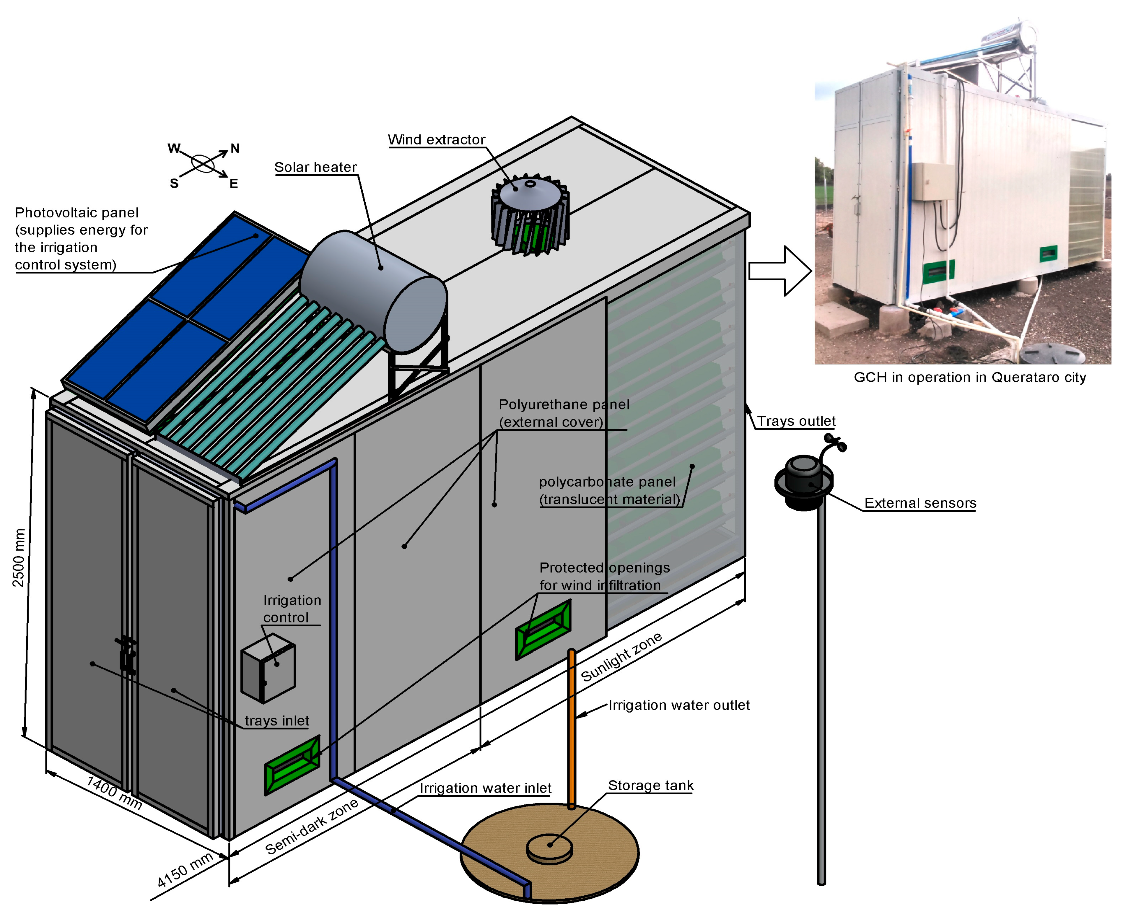
The development of mathematical models and their subsequent simulations are used to predict the behavior of certain variables in a determinate system that changes over time. In our case, such a system is the growth chamber (GCH) presented in Figure 1. Due to the complex interactions carried out among the variables, such as temperature, humidity, radiation, carbon dioxide, water, nutrients, pests, diseases, and weeds, among others, it is necessary to identify and analyze them in subsystems. Several authors [1,2,3,4,5,6,7,8,9,10,11,12,13,14,15,16,17,18,19,20] have characterized the subsystems from different perspectives—for example, climate, nutrition, and irrigation. Models are used to achieve detailed knowledge of all interactions and processes. In some research, through modeling and simulation, the effects of environmental control techniques are analyzed to maintain the following critical variables: Temperature, humidity, lighting, and carbon dioxide concentration [1,2]. Other research projects predict the behavior of one or more variables and provide an appropriate response to keep these variables within the desired limits [3,4,5]. Most of the research on modeling and simulations has mainly been developed for greenhouses [6,7,8,9,10,11] to predict the internal environmental conditions of enclosures utilized for cultivation and plant growth. Several studies from the perspective of different environments of models have also been pursued, with the objective of knowing the behavior of the internal variables, such as temperature and relative humidity, that will serve as support to later define an adequate strategy for controlling the growth conditions within an enclosure. Although the type of crop is not defined explicitly, its influence is implicit, given its inherent condition in the models. These studies have implemented different approaches to develop these models, such as neural networks, genetic algorithms, and neuro-fuzzy models [12,13,14,15,16], where the object of study centers on natural ventilation, forced ventilation, cooling evaporators, or systems that integrate calefaction [17,18,19,20], to mention a few of them. On the other hand, there are alternative studies not developed for greenhouse environments, and proposed by some authors to model and simulate temperature and humidity [21,22,23,24,25].
In our proposal, physical principles are used to obtain a mathematical model of the GCH. Due to this, its internal environment is described employing differential equations [26]. This methodology permits researchers to obtain an environmental model of the GCH, relating outside variables (air temperature, relative humidity, global radiation, and wind speed), inside variables (for example, evapotranspiration), and the optical and thermal properties of building materials, along with the volume and surface of the enclosure. In our research, the resolution of equations and the implementation of the simulations were carried out with Matlab® (R2010A, MathWorks, Natick, MA, USA) software.
In this study, the authors propose a novel GCH that integrates the concept of renewable energy taking advantage of natural resources for its operation because it uses a roof-mounted solar panel. Due to its design, the GCH uses a passive system to control temperature and humidity. The GCH does not contain artificial heating, cooling, or lighting systems, and might be relevant to the production of hydroponic green forage. A mathematical model has been developed to estimate the inside air temperature and relative humidity of the GCH. The confidence in the accuracy and reliability of the model is established comparing the simulated values and measured values through the coefficient of determination (R2), and the root mean squared error (RMSE). Results of the comparison reveal good agreement between experimental measurement data and those obtained by the mathematical model. It needs clarifying that it is not the main objective of the current research to develop a complex model with a high level of detail and accuracy, but a simple model that gives satisfactory predictions for realistic environmental responses of the air temperature and humidity inside the GCH. The application of the simulation results of this study may be regarded as a reference to optimize the prediction model of temperature and humidity in other growth chambers under study.

2. Materials and Methods

This research was carried out on a farm in Querétaro, México (20°32’57.4"N, 100°30’11.7"W), where the GCH is in the open air. To clarify the explanation, this section consists of the following four parts: (1) Growth chamber, in this part describes the camera and all its components; (2) Instrumentation and environmental data, which deals with the sensors used in the study, along with the equation to filter the information; (3) Environmental model, here the mathematical expressions corresponding to the equations of temperature and relative humidity are introduced to analyze the interior of the GCH; and (4) Initial conditions, in which the initial conditions are established to solve the differential equations.

2.1. Growth Chamber

This study centers on the prediction and measurement of the internal air temperature and relative humidity in a GCH built on a farm in the open air, in Querétaro, México.
Its purpose is the growth and development of temporary crops (TCs) of hydroponic green forage (HGF). It is worth mentioning that the crop term used in our work is employed according to the FAO definition (available from http://www.fao.org/es/faodef/fdef11e.htm), i.e., forage used mainly as part of the animal diet, and that can become temporary. Figure 1 presents the scheme of the proposed chamber, and a description is given as follows: Due to its design, the GCH uses passive systems to control the temperature, humidity, and wind speed based on filtering outside conditions without operating any climate control system (heating, cooling, or evaporative).
The GCH integrates the concept of renewable energy because it counts with technology that takes advantage of the natural resources for its operation. Furthermore, it is built with an anticorrosive metallic structure with a tubular rectangular profile in stainless steel of 40 × 40 mm, caliber 12, resulting in rigidity. Additionally, covered with a sandwich-type panel of galvanized steel metal faces and a rigid insulating core of high-density polyurethane PUR (40 kg·m−3) with a thickness of 40 mm, model PF600-40L of the company PAINEL2000, which is useful for isolating the interior from the extreme conditions of the elements. On the roof are placed a solar collector, a polycrystalline solar panel of the 125 W brand EPCOM model EPL12512, and a wind extractor brand ATCFANS model BK2000-14 of anodized aluminum. The photovoltaic system ensures the implementation and operation of the GCH anywhere, without relying on conventional electricity, complemented by the following three elements: (1) A solar charge controller with pulse width modulation (PMW), manufactured by PHOCOS model CX40; (2) a RALLY 1200 W inverter model 7466 to convert 12 V DC to 120 V AC; and (3) two solar batteries of a deep cycle of absorbent glass mat (AGM), brand CONER model 31H, 12 V, and 115 Ah. The extractor only rotates because of the external wind present in the GCH installation site (the movement of the wind extractor is ignored, due to the temperature differential). Therefore, ventilation is said to be natural. The lower part of each wall of the chamber (right and left) has two openings, with a stainless-steel mesh 40, SORFORD brand, that prevents the pests or objects entry since the GCH is outdoors. Due to the wind extractor, air enters through these openings and flows upwards. A high-density geomembrane (HDPE) of 1 mm thickness manufactured by GSE covers the wood floor.
The interior of the GCH is divided into two zones: The first part offers semi-dark conditions and must be kept like this during the first eight days, when the seed begins to germinate, and a second part, where the forage shoots are exposed to sunlight to complete their development from the ninth day to the fifteenth day. The lighting is natural thanks to the sun rays that cross the cellular polycarbonate panel (SKYFLEX U-profile 6 mm). In the interior of the GCH, there are 12 rails used to displace the trays horizontally, distributed in two sections, with six rails per section, and rails are separated vertically by 31 cm.
The growth of the HGF takes place in trays of 60 × 40 cm and 7.5 cm high, manufactured by HYDROCULTURA. Each tray has a 35.5° tilt angle with holes in the bottom, allowing water to flow and drain; unlike conventional production systems that use the practice of run and waste irrigation, i.e., the water on the floor is not reused and wasted. Besides, there is a system for the recirculation of water, which lets considerable water savings. This is one of the advantages of the proposed production system.
Additionally, the GCH has a system of irrigation with the following two components: (1) A storage tank of 1000 L, and (2) a submersible water pump of the 250 W brand ORANGEPUMPS model CSP250C-4. The distribution of the water is carried out with PVC tubes that are 13 mm in diameter, with perforations every 64 cm, where there are installed sprinklers manufactured by the EVERGREEN model MS 8009. The irrigation is conducted using pure water, without nutrients and fertilizers.
The GCH is defined as follows: The GCH is a prototype aimed at mitigating or preventing production losses for small and medium livestock producers, or producers of small animals. It has the following characteristics: It is a small chamber, people cannot walk inside it, and only a part of it contains translucent material. Thanks to its shape and size, the chamber can be relocated without disarming it in its entirety, and for its installation and startup, little time is required. The GCH makes efficient use of space due to the structure composed of several layers in a vertical direction. Due to the optimal isolation of the camera, it exhibits an efficient energy consumption.
On the other hand, one would think that a GCH is like a greenhouse; however, there are several differences. For example, a greenhouse is a closed, static, and accessible on foot, and the light crosses the translucent glass or the plastic, letting use of the effect of solar radiation. This structure covers the crop and has at least one device that can be manipulated to control the variables of the environment, nutritional or biotic or both, that influence the growth and development of the crop. Another marked difference between a greenhouse and the GCH is in the commercial aspect because a greenhouse seeks large-scale production that generates economic value, whereas a GCH is used to ensure the production of animal food.

2.2. Instrumentation and Environmental Data

The GCH counts with a temperature sensor and a data logger factory certified and calibrated brand EXTECH model RHT10.The sensor location is 2.08 m behind from the doors, 1.25 m above the floor, and 0.7 m in front of the walls. This device is useful to register and store temperature and relative humidity each day. The resolution and accuracy of the temperature sensor are 0.1 °C and ±1.0 °C, respectively. The resolution of the relative humidity sensor is 0.1%RH. The accuracy changes according to the range of measurement; for the range of 60 to 80%RH, it is of ±3.5%RH, and for 80 to 10%RH, it is of ±5.0%RH. The external weather conditions are obtained from a station Davis Vantage Pro weather, model 6162. This is located outside of the GCH, 4 m to the left from the wall and 3 m from the ground, and permits to capture the following data: Temperature, relative humidity, solar radiation, and wind speed.
In this study, data collected on 11 November 2015 and 2 February 2016 were used to carry out the characterization of the model for simulation purposes. These data were selected because when compared with the information obtained on the other days, they presented major disturbances. The temperature and humidity were acquired every 5 min (measurement interval), obtaining a total of 288 measurements per variable in a day. Other data collected during two consecutive weeks, from 3 July 2016 to 16 July 2016 (15 days were selected because this period corresponds to a cycle of production of HGF), were used to validate the model, i.e., 4320 measurements in 15 days per variable. This measurement interval for data collection was established based on the work reported in [2,8].
It is also worth mentioning that the recorded data were filtered to avoid unwanted peaks during the simulation process. The filter used is called median–mean, and it is useful in statistical analysis. This filter computes the mean filter first, followed by the median operator. Formally, this is expressed by:
ξ μ B ( f ) ( x ) = X M μ B ( X ¯ μ B ( f ) ) ( x )
where, ξ μ B represents the median–mean filter size µ; X M μ B is the median filter size µ; X ¯ μ B denotes the mean filter size µ; f represents the input vector; x is the evaluation point; B symbolizes the elemental structuring element; and µ is a size criterion, e.g., if µ = 1, the number of elements is 2µ + 1 = 3, and if µ = 2, then the number of elements is 2µ + 1 = 5, etc. The filter expressed in Equation (1) was implemented in Matlab® R2010A.

2.3. Environmental Model

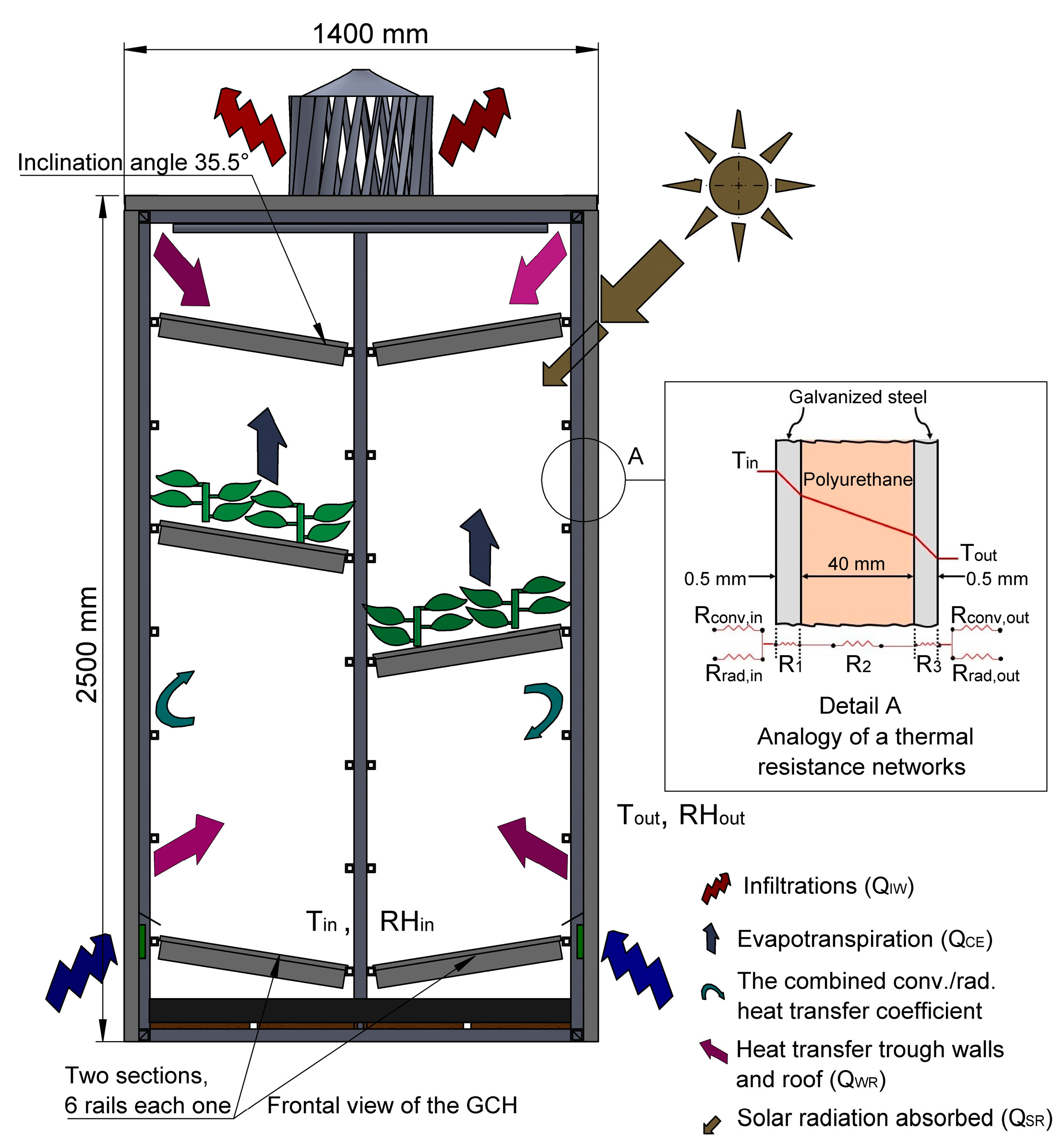
The internal environment of the GCH can be described using a system of two differential equations of the first order, which characterize the behavior of the air temperature and relative humidity [21,27,28] following the mass and energy balances considering the interactions illustrated in Figure 2. External climatic conditions influence this model, as well as the location, orientation, and size of the GCH. The simplified environmental model described in this section takes into consideration next assumptions:
(1) In the temperature model of the air, the heat sources are the heat absorbed through the translucent surfaces, the evapotranspiration of the TC, and the heat transfer through walls and ceiling, while the main source of heat loss is the ventilation. The condensation of the walls (as a result of latent heat) is considered as a parameter neither the water nebulization nor evaporation on the surface of the soil.
(2) The model of humidity in the air considers the evapotranspiration of the crop and ventilation as the main cause of humidity gain and loss, respectively.
(3) The crop evapotranspiration variable utilized in the environmental model comes from some relationships proposed by other authors. Such variables satisfy to be a linear function of the global radiation.
(4) The mathematical relationships of physical processes such as ventilation are simplified. The wind speed within the GCH is considered homogeneous, without considering the multiple crop layers in the GCH. Natural ventilation temperature is despised, due to the small effect of it, with respect to that produced for the wind. Empirical relationships are used to model this physical phenomenon.
(5) The internal temperature and humidity models consider a uniform homogeneous distribution of variables inside the GCH.

2.3.1. The Internal Air Temperature Model

Figure 2 illustrates that the GCH gains heat due to solar radiation absorbed through the translucent surfaces (QSR), the heat provided by crop evapotranspiration (QCE), and the heat transfer through walls and roof (QWR), while the heat losses are due to infiltrations and the effect of wind (QIW). The equation proposed for modeling the behavior of the internal temperature is the following:
d T i n d t = 1 C p ρ a H [ Q S R + Q C E + Q W R Q I W ]
where c p is the specific heat at constant pressure ( J · kg dry   air 1 · K 1 ), ρ a is the air density ( kg dry   air · m 3 ), H represents the average height of the GCH (m).
The heat absorbed by the translucent surface of the GCH due to solar radiation is estimated using the next equation [29,30]:
Q S R = C 1 Q G R
where Q G R is the external global radiation (W∙m−2), and C 1 is a dimensionless coefficient that relates to the energy transmittance through the translucent material and it is a property of the materials used during its construction.
According to the literature, there are several mathematical models of evapotranspiration for crops [31,32,33], some of which are more complex than others. However, the factor that has demonstrated the highest correlation with evapotranspiration is radiation. Based on the work carried out by Jolliet [34], we assume that crop evapotranspiration is a linear function of solar radiation. For this reason, Equation (4) expresses the term that associates the heat contributed by evapotranspiration ( Q C E ) [29]:
Q C E = E = 0.00006 C 1 Q G R + 0.0004
The heat gain through the walls and the ceiling to the interior of the GCH (QWR) consider (1) the conduction through the wall and roof, and (2) the convection and radiation associated with its surfaces. Equation (5) is defined as [35]:
Q W R = ( T i n T o u t ) R t o t a l
where   T i n T o u t , defines the temperature difference between inside and outside of the GCH, R t o t a l is the total thermal resistance in m 2 · · W 1 . Q W R can be handled using the thermal resistance concept. Figure 2 (Detail A) illustrates the analogy of the thermal resistance networks.
The Equations (6)–(11) represent the concept of the thermal resistance parameter. This concept is employed, e.g., by Sarafraz et al. [36], for estimating the overall heat transfer coefficient ( 1 / R ). The equations defined in [35] are presented as follows:
R c o n v ,   i n = 1 h c o n v ,   i n
R r a d ,   i n = 1 h r a d ,   i n = ε · σ · ( T c o v ,   i n 2 + T i n 2 ) · ( T c o v ,   i n + T i n )
R 1 = R 3 = 1.80   m 2 · · W 1
R 2 = R P u l = b K m a t
R c o n v ,   o u t = 1 h c o n v ,   o u t
R c o n v ,   o u t = 1 h r a d ,   o u t = ε · σ · ( T c o v ,   o u t 2 + T i n 2 ) · ( T c o v ,   o u t + T i n )
where   h c o n v and h r a d are the convection and radiation heat transfer coefficients at the surfaces; ε is the emissivity coefficient; σ corresponds to the Stefan–Boltzmann constant; T c o v ,   i n T c o v ,   o u t are the temperatures in the interior and the outside surfaces, respectively; R 1 represents the thermal resistance for the inner and outer sheets of the galvanized steel metal faces with a thickness of 0.5 mm, respectively; b is the thickness of the insulating core; K m a t is the declared thermal conductivity with a value of 0.0211   W · m 1 · 1 . The values are in the technical data sheet of the materials.
Since the convection and radiation resistances are parallel to each other, this may cause some complications in the thermal resistance network. By replacing h c o n v in Equations (6) and (10) by h c o n v ,   r a d ,   i n and h c o n v ,   r a d ,   o u t , which include the effects of radiation on the inner and outer sheets of the galvanized steel metal surfaces of walls and roofs (called surface conductance, which represents the combined convection and radiation heat transfer coefficients), avoids all the complications associated with radiation effect. The common values for h c o n v ,   r a d ,   i n and h c o n v ,   r a d ,   o u t , considering a maximum load, are computed as follows [37]:
h c o n v ,   r a d ,   i n = 8.29   W · m 2 · 1     ( summer   or   winter )
h c o n v ,   r a d ,   o u t = { 34.0   W · m 2 · 1     ( winter ) 22.7   W · m 2 · 1     ( summer )  
According to the consideration made for the radiation effect, the resistance configuration is in series, hence the total thermal resistance is obtained below:
R t o t a l = R c o n v ,   r a d ,   i n + R 1 + R P u l + R 3 + R c o n v ,   r a d ,   o u t
The energy flow caused by infiltrations and the effect of ventilation is computed below [30]:
Q I W = φ w i n d   ρ a c p A   L C ( T i n T o u t )
where φ w i n d   represents the airflow through the apertures of the GCH (m3∙s−1), and A L C is the longitudinal area of the camera ( m 2 ), which is the result of multiplying the width by the height of the GCH.
Subsequently, when replacing Equations (3)–(5) and (15) in Equation (2), the mathematical model to predict the internal air temperature of the GCH is:
d T i n d t = 1 C p · ρ a · H {   ( C 1 · Q G R ) + ( 0.00006 · C 1 · Q G R + 0.0004 ) + ( T i n T o u t ) R t o t a l φ w i n d   · ρ a · c p A   L C ( T i n T o u t ) }

2.3.2. The Internal Air Relative Humidity Model

For the relative humidity, the source of water vapor was evapotranspiration from TC (E), and the only water loss from the system was due to ventilation. Then, Equation (17) represents the changes in water vapor produced inside the GCH, i.e.,
d ω i n d t = 1 H ρ a [ E φ w i n d   A L C ρ a ( ω i n ω o u t ) ]
Equation (4) establishes the crop evapotranspiration E ( kg water ∙m−2∙s−1), ω i n ω o u t represents the difference between the inside and outside absolute humidity of the GCH, and it is calculated utilizing the next equations [38]:
ω i n =   R H i n 100 [ ( 0.004055 ) + ( 0.0001152 · T i n   s i m ) + ( 0.00002167 · T i n   s i m 2 ) ]
ω o u t =   R H o u t 100 [ ( 0.004055 ) + ( 0.0001152 · T o u t ) + ( 0.00002167 · T o u t   2 ) ]
where R H i n is the internal relative humidity of the chamber, and T i n   s i m is the value simulated by the temperature obtained through Equation (16).
2.4. Initial Conditions

The initial conditions (time t = 0) for each one of the state variables of the differential Equations (12) and (14) were assumed to be equal to the measured outside temperature ( T o u t ) and humidity ( ω o u t ). For instance, when recording measurement data at the time 00:00, with the outside temperature sensor reading 15 °C, then T i n   =   T o u t   =   15   ° C ; similarly, it is done for ω i n   =   ω o u t . Other initial input values used in these equations were the outside measured variables, such as global radiation and wind speed. Table 1 presents the parameters used in the model.

3. Results

To evaluate the performance of the mathematical model, we used two criteria: (1) The coefficient of determination (R2) obtained through a regression analysis (for the humidity, a fifth-degree polynomial function is used, due to the nonlinear behavior), and (2) the root means squared error (RMSE). These criteria assessed the correlation between simulated and measured values. They are defined as follows:
RMSE   T   ( ° C ) = 1 n 1 n ( T i n   s i m T i n   m e a ) 2
RMSE   R H   ( % ) = 1 n 1 n ( R H i n   s i m R H i n   m e a ) 2
where T i n   s i m and R H i n   s i m correspond to the simulated values of the temperature and the relative humidity inside the GCH, respectively, and T i n   m e a and R H i n   m e a represent the measured values of the temperature and the relative humidity inside the GCH, respectively.
The uncertainties of the experimental results are obtained using the Kline-McClintock equation [39] employed in [36]. Based on the uncertainty analysis, the uncertainties of the T i n   s i m and R H i n   s i m are 12.8% and 8.1%.
The results section consists of the following four parts: (1) Two days are analyzed in different seasons. The parameter R2 is computed analyzing the differences between the measured and simulated data; (2) parameters RMSE and R2 are obtained using the data of two consecutive weeks corresponding to the summer season; (3) internal conditions of the GCH, where a percentage is computed to know how much the temperature and humidity maintain ideal conditions without operating any heating or cooling system; and (4) GCH operation example. Here is illustrated the practical functionality of the proposed GCH.

3.1. Two Days in Different Seasons

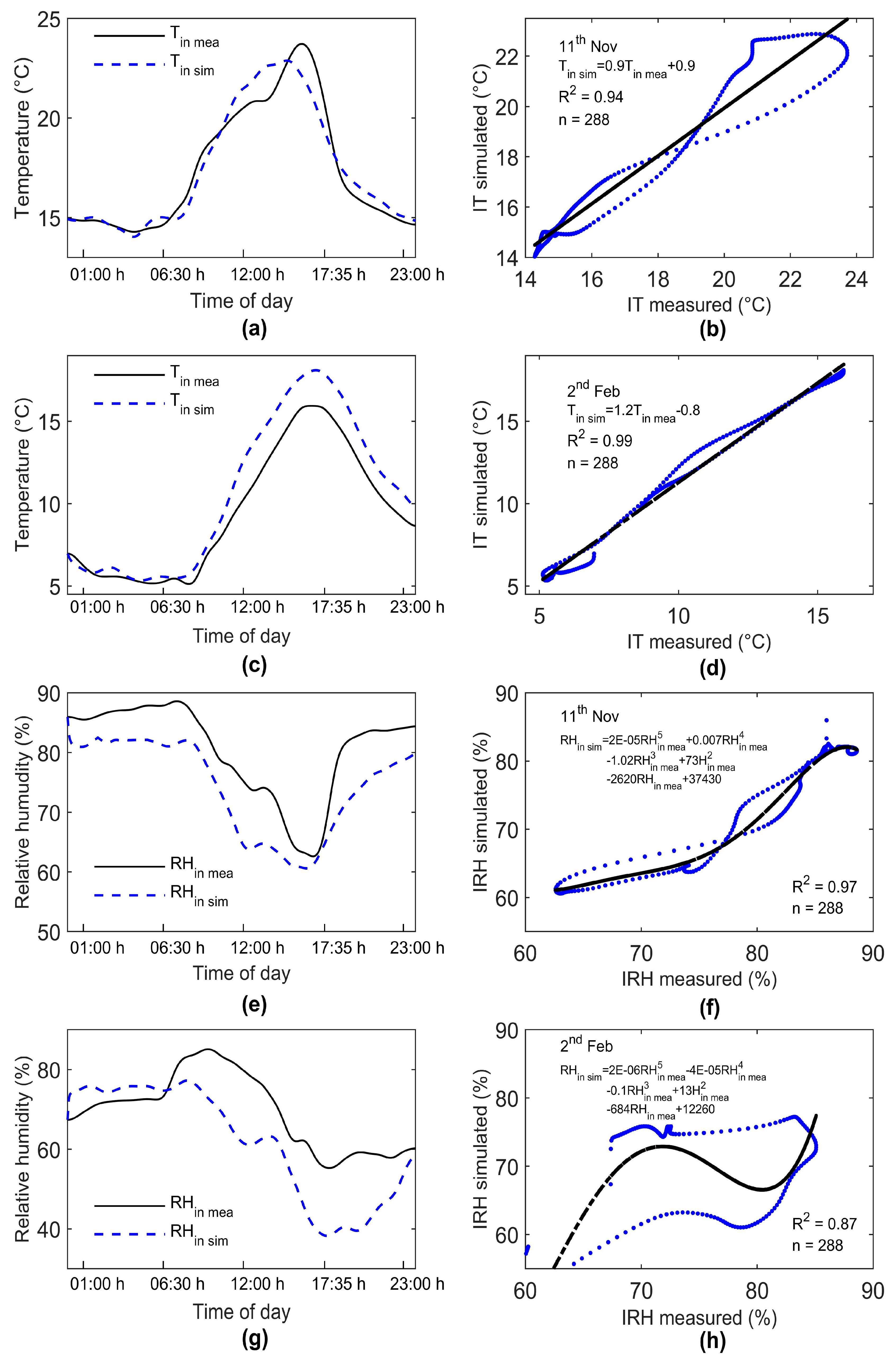
The results of the simulation corresponding to the temperature and relative humidity of two days, 11 November 2015 and 2 February 2016, can be seen in Figure 3a,c,e,g, respectively. For each day are taken into account 288 samples of temperature and relative humidity, 1152 samples are considered in total. From the data graphed in Figure 3, the average difference between the simulated value and the measured value is computed, giving a result of T i n   s i m T i n   m e a ¯ = 0.06 °C for the temperature and R H i n   s i m R H i n   m e a ¯ = −6.1%RH for the relative humidity on a day in autumn, and T i n   s i m T i n   m e a ¯ = 1.2 °C and R H i n   s i m R H i n   m e a ¯ = −7.9%RH for a winter day. Negative signs reveal an underestimation of the mathematical model, i.e., the simulated value was less than the measured value.
Figure 3b,d,f,h shows the graphs corresponding to regression analysis for the two days considered in the simulation. The coefficients of determination deduced from the data are the following: (1) R2 = 0.94 for the temperatures on an autumn day and R2 = 0.99 for temperatures on a winter day, and (2) R2 = 0.97 for the relative humidity on an autumn day and R2 = 0.87 for the relative humidity on a winter day. Comparing the coefficients obtained in this research concerning those reported in [40], whose values are R2 = 0.92 and R2 = 0.87 for the temperature and relative humidity in a greenhouse, a little improvement was observed in respect to the temperature, and no difference to the relative humidity.

3.2. Two Consecutive Weeks

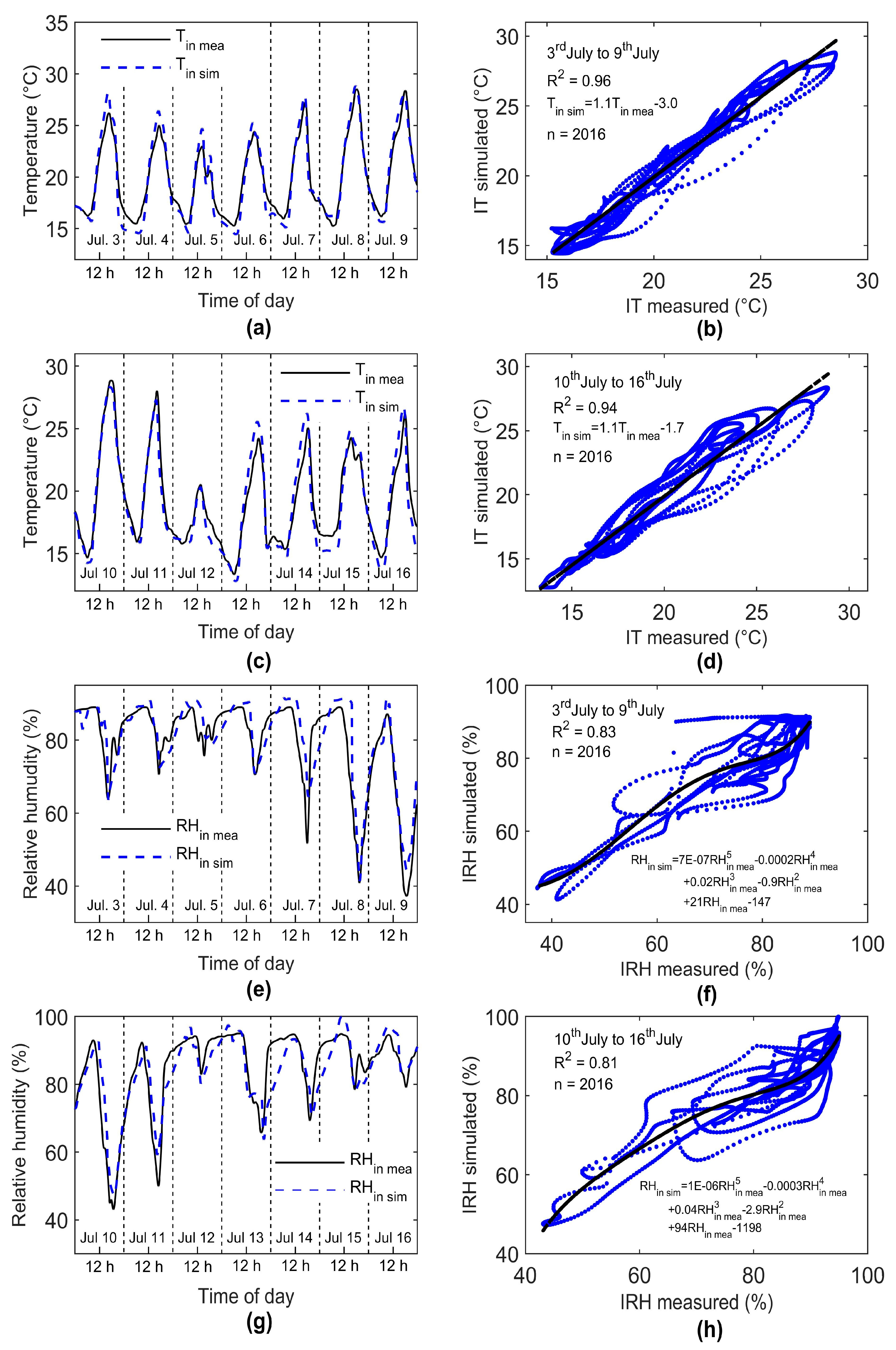
Similar simulations to those presented in Figure 3 are provided in this section, but now considering 15 days. In Figure 4, the corresponding graphs for the temperature (n = 2016) and relative humidity (n = 2016) for the two weeks (from 3 July 2016 to 16 July 2016) are displayed. In Figure 4, the horizontal lines indicate the days. Figure 4a,c shows a visual check of the measured internal temperature and the simulated (or predicted) internal temperature of the week from July 3 to 9 (first week) and the week from July 10 to 16 (second week), respectively. Figure 4b,d shows the internal temperature regression analysis, with the regression lines that best adjust to the scatter diagram and the linear regression equations with their coefficient of determination values. Similarly, Figure 4e,g shows a visual check of the measured internal relative humidity, and the simulated (or predicted) internal relative humidity of the first and the second week, respectively. Figure 4f,h shows the internal relative humidity regression analysis using a polynomial approximation (to get a best adjust of the data), with the regression lines that best adjust to the scatter diagram and the regression equations with their coefficient of determination values. The RMSE values for the first week are 0.98 °C and 5.5%RH, whereas those for the second week are 1.08 °C and 5.5%RH. In the same way, the RMSE value of the simulated temperature is less than the value reported in [15], of 1.9 °C, and a bit higher than the RMSE value of the relative humidity reported in the same paper, with a value of 3.2%RH for three consecutive days in a greenhouse. The computed RMSE value obtained in our research is slightly higher than that reported in [26], of 0.9 °C, and lower when compared to the relative humidity of 6.6%RH for a single day of simulation inside a greenhouse.
Table 2 presents the coefficient of determination and the mean squared errors associated with the obtained simulations through the proposed humidity model, and those obtained from a humidity model that includes (i) a different method to obtain evapotranspiration [32], and (ii) an equation for condensation [41]. In Appendix A, the tests under different scenarios using the mathematical model are presented.
In several studies [6,40], the regression analysis applied to the model has as a linear correspondence, but in our case, due to the fluctuations presented by the data, a polynomial approximation is computed since the behavior does not correspond with a straight line. Table 3 shows the R2 values calculated using linear regression and a fifth-degree polynomial.
In Appendix B, the units of Equations (2) and (17) are verified.

3.3. Internal Conditions of the GCH

The variables that most influence the development of the TC of the HGF are temperature and humidity. In the literature, several studies have been carried out under different conditions of controlled temperature and relative humidity, depending on the application—for example, 21–25 °C and 65–75%RH [42]; 22–26 °C and 50–73%RH [43]; 23–25 °C and 6–70%RH [44]; 18–21 °C and 70%RH [45]. In such studies are reported yields of 7–12 kg of wet HGF per kilogram of harvested seed. The temperature and humidity must keep as stable as possible within a specific range to obtain a good crop inside the GCH. If we establish the ideal range for internal conditions (temperature and humidity), based on the previously cited authors, which is between 20 °C and 25 °C for temperature and 70% and 80% for relative humidity, we find that only 31% of the temperature data measured inside the chamber remain in that ideal internal temperature range, although the average internal temperature measured is 20 °C. In the case of relative humidity, only 14% of the humidity data measured inside the chamber are in the ideal humidity range, while the average of internal relative humidity measured is 82%.

3.4. GCH Operation Example

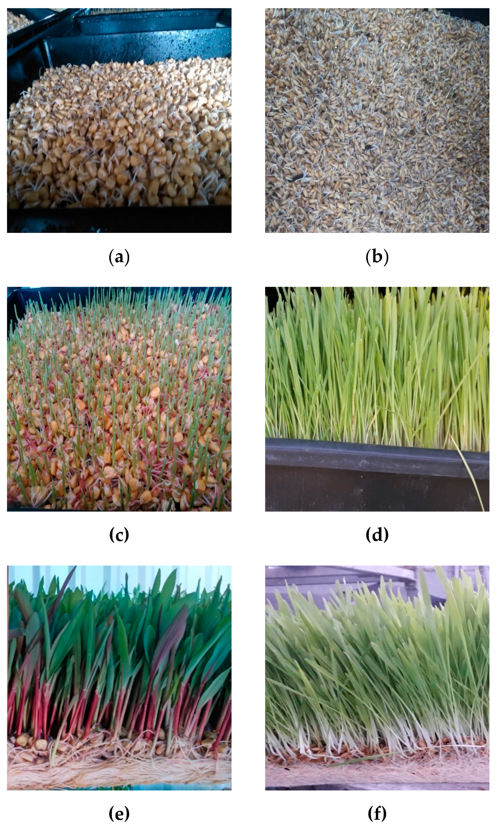
The TC examples provided in this subsection serve uniquely to illustrate the functionality of the proposed GCH. This paper just reports the results obtained in the field of forage production using the GCH. Our approach is the modeling and simulation of the internal air temperature and internal relative humidity. In this way, any economic, practical, or nutritional analysis is outside of the scope of the paper. The TCs correspond to the Zea mays and Hordeum vulgare in production cycles of 15 days and 12 days, respectively. The total water used inside the chamber has been generally defined in agronomy [44] as the water added during the irrigation minus the water drained out of the trays. The amount of water used to produce a daily average of forage is equal to the kilograms of wet forage produced on average daily by the GCH among the total water used inside the chamber. Due to the use of recirculation system water, the GCH can produce HGF while saving water. On average, it produces 1.4 kg of corn HGF and 1.7 kg of barley HGF using a liter of water per day in cycles of 15 and 12 days, respectively. Figure 5 illustrates a comparison of the HGF production from Zea mays and Hordeum vulgare. Additionally, the mass of the seed at the time of harvesting (wet seed after being immersed in water for 48 hours) was registered. During the seeding procedure, the seed was weighed dry and recorded. Another measure considered was the mass of wet forage at the time of being recollected. In Appendix C, there are further details on the obtention of HGF.
Table 4 provides information about the kilograms of wet forage obtained for a TC of corn in a cycle of 15 days. Equally, in Table 5, the results for a TC of barley in a cycle of 12 days are presented. The conversion factor relates dry seed to fresh forage of the same sample produced in the GCH, and differs from the conversion ratio (CR), which considers the concentration of dry matter.
A conversion factor of 3.5 is obtained on average, i.e., 3.5 kg of fresh HGF is produced for each kilogram of dry seed planted. The GCH presented in this paper only fulfills the specified objectives, and there is not any interest to carry out a commercial or economic analysis. The performance is low when compared with the results reported in [45], with respect to the proposed hydroponic system, which presented values between 4.93 kg and 7.21 kg of fresh forage for each kilogram of barley grain. In [42], 1 kg of forage seed produces a quantity of wet forage between 7 kg and 9 kg. This occurs because the seed utilized in our project is not certified. Therefore, the percentage of germination is unknown; besides, irrigation was carried out using pure water.

4. Discussion

The results of the model give satisfactory predictions for the air temperature and the humidity in the GCH. Overestimation during the day and underestimation during the night may be due to the unsuitable consideration of a heat transfer coefficient for walls-air or crop-air. Due to the fact that the value of relative humidity depends on the internal airflow through the apertures of the GCH (φwind) and the evapotranspiration inside of the GCH ( E ), which is not measured directly in this research, they are only estimated using equations that were developed with experimental data for different conditions than those used in this study.
The results obtained with the proposed humidity model were compared with another system that includes (i) a different method of calculating evapotranspiration [32], and (ii) an equation for condensation [41]. This comparison shows that there are no significant differences in the R2 parameters obtained by both methods. Our results are similar when applying the mathematical model proposed by Hargreaves [32] where, the authors do not consider analyzing samples in short lapses of time; in our case, every 5 minutes, radiation was measured—i.e., variations of temperature occur in a longer time, at the beginning and the end of the day, instead of a sampling period. While the equation proposed here is not general, it can be used to compute determined parameters using the captured information of solar radiation. On the other hand, the model introduced by Hargreaves [32] employs tabulated values derived from other experimental procedures.
Moreover, Cengel and Boles [46] have affirmed that, contrary to the relative humidity that varies as the temperature varies, the absolute humidity remains constant in the presence of these variations. Since the estimation of it is performed using absolute humidity, the results may not reflect the variations that relative humidity would display, and this could explain the low coefficient of determination values for the humidity model.
Similarly, from the point cloud shown in the scatter diagrams for the humidity model in Figure 3f,h and Figure 4f,h, there is a better correspondence between the simulated values and the measured values with a nonlinear function. According to that expressed in [25] and [15], relative humidity is a nonlinear phenomenon because nonlinear equations involved in its modeling govern the transfer of heat and mass. Therefore, linear models like ours suffer from many of the shortcomings by not considering nonlinear effects.
Besides, two factors we have considered for explaining the deviation remaining between the values simulated by the model and the measurements are the following: (1) The complexity of choosing the correct calibration parameters that allow all the state variables that are involved in the model to be adjusted simultaneously, and (2) the assumption that the GCH is a perfect mixing tank, when in fact, the air movement is somewhat limited as a result of the multiple trays inside the GCH. This impacts on the temperature and moisture distribution inside the chamber, since we assume that the air is like a perfectly mixed fluid when there is a spatial distribution.
The simulated data and the values measured experimentally have a good fit. However, the model can be improved. Nevertheless, the use of more complex equations to model humidity within cultivated enclosures does not guarantee better results. For example, in [6], the authors obtained lower coefficients of determination than ours, or the research reported in [40], who obtained slightly higher coefficients than ours. It is so complex to model humidity conditions, that there are even authors who, in their work, only model and simulate temperature, or perhaps they do not show interest in this [11,15,28,30,38].
For 11 November, which corresponds to the autumn season, the measured maximum difference between the internal air temperature of the chamber T i n and the external temperature T o u t was 2.27 °C. However, on average, the internal air temperature was only 0.01 °C lower than the external temperature. In the case of relative humidity, the measured maximum difference between the internal relative humidity ( ϕ i n ) and external relative humidity ( ϕ o u t ) was 20.8%. The internal relative humidity was 11.5% higher than the external relative humidity on average. On 2 February, corresponding to the winter season, the measured maximum difference between the internal air temperature of the chamber and the external temperature was 0.69 °C. However, the internal temperature remains 1.1 °C lower than the external temperature on average. On the other hand, the maximum difference between the internal relative humidity of the chamber and the external relative humidity was 33.2%, and the internal humidity was 11.5% higher than the external humidity on average. In the case of the summer season, two consecutive weeks from 3 July to 16 July were analyzed, the measured maximum differences between the interior and exterior of the chamber were 3.82 °C and 38.8% for temperature and relative humidity, respectively. Similarly, the internal air temperature was only higher than the external temperature by an average of 0.34 °C, and the internal relative humidity was maintained at an average of 15.7% higher than the external humidity.
On the other hand, the R2 data computed with values 0.96 and 0.94 for the temperature model and of 0.81 and 0.80 for the humidity model for two consecutive weeks are not necessarily bad when compared, concerning other index values published in other papers. For example, in the research presented in [6], the R2 values computed for the internal air temperature were 0.89, 0.80, and 0.80; similarly, R2 values of 0.52, 0.73, and 0.77 were obtained for simulated humidity in several runs. As can be seen, these R2 values are lower than those obtained by the model proposed in this paper. Another example is presented in [40], who obtained an R2 maximum of 0.92 for the internal temperature and 0.87 for the internal relative humidity. These results are slightly higher than those reported in our research. Notice that the R2 value of 0.80 is quite common among the published works, which derives from the complexity to predict humidity in closed enclosures for crops.

5. Conclusions

The simple and efficient mathematical model proposed in this paper to predict the internal air temperature and relative humidity is a useful tool to know the behavior of these variables within the GCH since, from the obtained results, the predicted values present a good correlation with the measured values and with those reported in the literature when comparing the R2 and RMSE parameters. The simulation results of this study are useful for the design and optimization of environmental control systems applied to a growth chamber. Next, some conclusions from the results are presented:
(1) During two consecutive weeks of the summer, the coefficients of determination values were R2 = 0.96 and R2 = 0.94 for the model of temperature, and R2 = 0.83 and R2 = 0.81 for the model of the relative humidity. For a winter day, these coefficients were R2 = 0.99 and R2 = 0.87 for air temperature and relative humidity, respectively. Similarly, the results for an autumn day were R2 = 0.94 and R2 = 0.97.
(2) The RMSE values for the temperature model were 0.98 (°C) and 1.08 (°C) during two consecutive weeks of summer, and 5.45 (%RH) and 5.48 (%RH) for the model of the humidity in the same period of measure. For an autumn day, the RMSE values computed were 0.78 (°C) and 6.5 (%RH) for temperature and humidity, respectively. For a winter day, the RMSE values were 1.47 (°C) and 11.6 (%RH).
(3) The average temperature differences between the simulated and measured air temperatures and simulated and measured relative humidity were no less than 0.1 °C and 1.2%RH for the period from the 3 to 9 July, and for the period from the 10 to 16 July, the differences were no less than 0.2 °C and less than 0.7%RH. Equally, the average differences were more than 0.06 °C (below the resolution of the sensor) and 6.1%RH, corresponding to an autumn day, and for a winter day, the results were no more than 1.2 °C and less than 7.9%RH.
(4) With the use of GCH, the growth of forage in different places and times of the year can be guaranteed, regardless of climatic conditions. Although the interior of the chamber, on average, was only a little colder in autumn ( ( T i n T o u t ) ¯ = 0.01   ° C , below the resolution of the sensor) and winter ( ( T i n T o u t ) ¯ = 1.1   ° C ) and only slightly hotter in summer ( ( T i n T o u t ) ¯ = + 0.3   ° C ), this did not prevent it from fulfilling its objective of producing HGF. It is worth emphasizing that the interior was always wet compared to the external conditions that occurred in the place of experimentation, so materials selected for the construction of the GCH are adequate.
(5) The results obtained in the production of HGF are interesting because, despite not having an environmental control, not using certified seed, and using water without nutrients, the average production rate of 3.5 kg of wet HGF was achieved for each kilogram of seed (corn or barley) harvested.

Author Contributions

G.D.-F. performed the experiments and wrote the paper. J.M.-S. supervised the experiments and analyzed the data. L.S.-S. revised and edited the paper. D.G.-M. contributed with the materials and original draft preparation. I.T.-V. revised and edited the paper. H.G.-B. revised and edited the paper. M.A.-E. revised and edited the paper. G.E.-G. obtained the resources. J.G.-E. revised and edited the manuscript. C.O.-O. supervised and managed the project.

Funding

This research received no external funding.

Acknowledgments

The authors thank CONACYT for the scholarship number 326183 and the Master´s program in Engineering Sciences SEP-CONACYT-PNPC-2852. The authors also thank the IDGREEN company for providing the use of their facilities.

Conflicts of Interest

The authors declare no conflicts of interest.

Appendix A

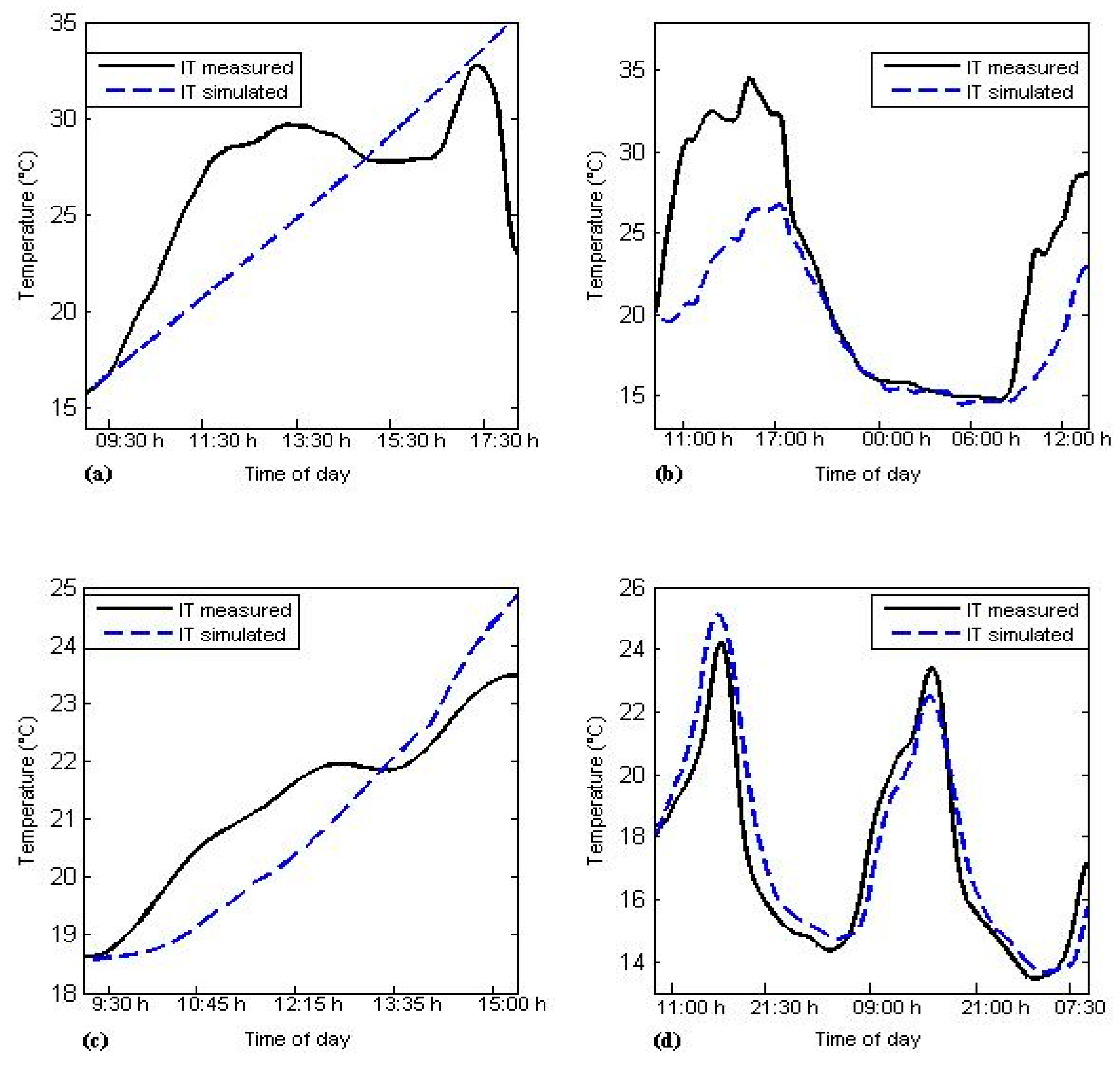
Four scenarios are presented below, considering the variables QSR, QWR, QIW, and QCE. They are added gradually until all of them are completed.
The first scenario, the temperature action does not consider ventilation, irrigation, or forage inside the GCH, i.e., only the heat flowing through the walls, ceilings, and translucent surfaces intervene. Figure A1a present the result, and Equation (2) is written as follows:
d T i n d t = 1 C p ρ a H { C 1 Q G R + ( T i n T o u t ) R t o t a l } ,
In the second scenario, natural ventilation without applying irrigation and forage is considered. Here, the variable that relates to the losses due to infiltrations of ventilation intervenes. In Figure A1b, is presented the result, and Equation (2) is expressed as:
d T i n d t = 1 C p ρ a H { C 1 Q G R + ( T i n T o u t ) R t o t a l φ w i n d   ρ a c p A   L C ( T i n T o u t ) } ,
In the first and second scenarios, an empty GCH is analyzed, so the heat provided by crop evapotranspiration does not intervene.
Third and fourth scenarios: These include all the variables and the contribution from crop evapotranspiration. The results are displayed in Figure A1c,d, respectively. Notice that better simulations occur when increasing the variable number and this indicates that at least four inputs are necessary for the development of a general model. Table A1 shows the coefficients of determination and the variables that intervene in each one of the scenarios.
Figure A1. Model behavior in multiple scenarios. (a) The first scenario, where the growth chamber is empty. (b) The second scenario, where only is considered natural ventilation. (c,d) Third and fourth scenarios, when all variables in the simulation are included.
Energies 12 04056 g0a1
Table A1. Comparison of simulated and measured values under different scenarios.
ScenariosR2RMSEVariablesData NumberDate
10.534.15QSR and QWR553, every minute8 August 2015
20.825.04QSR, QWR, and QIW1722, every minute20 to 21 August 2015
30.860.92QSR, QWR, QIW, and QCE75, every five minutes11 August 2015
40.911.04QSR, QWR, QIW, and QCE582, every five minutes12 to 14 November 2015

Appendix B

In this appendix the units of Equations (2) and (17) of the mathematical model are explained in detail.
d T i n d t = 1 C p ρ a H [ Q S R + Q C E + Q W R Q I W ] ,
d ω i n d t =   1 H ρ a [ E φ w i n d   A L C ρ a ( ω i n ω o u t ) ] ,
Table A2. Units of the equations.
ParameterDescriptionUnits
Q S R C 1 Q G R W m 2
Q C E 0.00006 C 1 Q G R + 0.0004 W m 2
Q W R ( T i n T o u t ) R t o t a l ( W m 2 · ) ( ) = W m 2
Q I W φ w i n d   ρ a c p A   L C ( T i n T o u t ) ( m 3 s · kg m 3 · J kg   K m 2 ) ( K ) = J s · m 2 = W m 2
E defined as a linear function of global radiation kg wat   vap m 2 · s
ω i n ω o u t relationship between the amount of water vapor contained in a unit of dry air mass kg wat   vap kg dry   air
φ w i n d   represents the air flow through the apertures of the GCH m 3 s
ρ a air density kg dry   air m 3
C p specific heat at constant pressure J kg · K
H average height of the GCH m
Now, we replace the units of each parameter in Equation (2):
d T i n d t = 1 J kg   K · kg m 3 · m · [ ( W m 2 + W m 2 + W m 2 ) W m 2 ]
d T i n d t = K · m 2 J · ( W m 2 )
It should be remembered that when W = J s , then
d T i n d t = K · m 2 J · ( J s · 1 m 2 )
d T i n d t = K s
For Equation (17), we have
d ω i n d t = 1 m · kg dry   air m 3 ( kg wat   vap m 2 · s )
d ω i n d t = m 2 kg dry   air · kg wat   vap m 2 · s
d ω i n d t = 1 s · kg wat   vap kg dry   air

Appendix C

Appendix C describes the seeding procedure. Consider maize seed (Zea mays) in a production cycle of 15 days. The process of the production of HGF was carried out through the following procedure: (1) Screening the seed: The seed was sieved to eliminate foreign agents; (2) cleaning of the seed: Impurities and fragments of seed not removed with the sieve were manually eliminated; (3) disinfecting and washing: Seeds were washed using tap water, and they were immersed posteriorly, in a solution of sodium hypochlorite for 10 min; (4) seed immersion: Corn seed was soaked in a container with water for 48 h to speed up germination, and posteriorly, water was changed after 24 h; (5) sowing in trays: The seed was moved to the cleaned and disinfected plastic trays and distributed without exceeding 1 cm in height; (6) harvesting: Once the trays contained the seeds, they were transported immediately to the interior of the GCH. The trays were situated in a semi-dark place on the rails (see Figure 1), advancing horizontally every time when placed inside; (7) irrigation: The micro-sprinklers were activated for 2 minutes each, with a total of eight irrigations per day; (8) growth: From the third day, the buds of the seedlings started growing, until completing their cycle on the fifteenth day.
During the production cycle, the variables of interest, humidity, and temperature in the GCH were collected.

References

  1. Bennis, N.; Duplaix, J.; Énéa, G.; Haloua, M.; Youlal, H. Greenhouse climate modelling and robust control. Comput. Electron. Agric. 2008, 61, 96–107. [Google Scholar] [CrossRef]
  2. Van Beveren, P.; Bontsema, J.; Van Straten, G.; Van Henten, E. Optimal control of greenhouse climate using minimal energy and grower defined bounds. Appl. Energy 2015, 159, 509–519. [Google Scholar] [CrossRef]
  3. Van Straten, G.; Challa, H.; Buwalda, F. Towards user accepted optimal control of greenhouse climate. Comput. Electron. Agric. 2000, 26, 221–238. [Google Scholar] [CrossRef]
  4. Van Straten, G.; Van Willigenburg, G.; Van Henten, E.; Van Ooteghem, R. Optimal Control of Greenhouse Cultivation; CRC Press: Boca Raton, FL, USA, 2010. [Google Scholar]
  5. Rodríguez, F.; Berenguel, M.; Guzmán, J.; Ramírez-Arias, A. Modeling and Control of Greenhouse Crop Growth; Springer: Berlin/Heidelberg, Germany, 2016. [Google Scholar]
  6. Luo, W.; De Zwart, H.F.; Daii, J.; Wang, X.; Stanghellini, C.; Bu, C. Simulation of Greenhouse Management in the Subtropics, Part I: Model Validation and Scenario Study for the Winter Season. Biosyst. Eng. 2005, 90, 307–318. [Google Scholar] [CrossRef]
  7. Carlini, M.; Castellucci, S. Modelling and Simulation for Energy Production Parametric Dependence in Greenhouses. Math. Probl. Eng. 2010, 2010, 1–28. [Google Scholar] [CrossRef] [Green Version]
  8. He, F.; Ma, C. Modeling greenhouse air humidity by means of artificial neural network and principal component analysis. Comput. Electron. Agric. 2010, 71, S19–S23. [Google Scholar] [CrossRef]
  9. Nebbali, R.; Roy, J.; Boulard, T. Dynamic simulation of the distributed radiative and convective climate within a cropped greenhouse. Renew. Energy 2012, 43, 111–129. [Google Scholar] [CrossRef]
  10. Kıyan, M.; Bingöl, E.; Melikoğlu, M.; Albostan, A. Modelling and simulation of a hybrid solar heating system for greenhouse applications using Matlab/Simulink. Energy Convers. Manag. 2013, 72, 147–155. [Google Scholar] [CrossRef]
  11. Guo, J.; Liu, Y.; Lü, E. Numerical Simulation of Temperature Decrease in Greenhouses with Summer Water-Sprinkling Roof. Energies 2019, 12, 2435. [Google Scholar] [CrossRef]
  12. Linker, R.; Seginer, I. Greenhouse temperature modeling: A comparison between sigmoid neural networks and hybrid models. Math. Comput. Simul. 2004, 65, 19–29. [Google Scholar] [CrossRef]
  13. Coelho, J.P.; Oliveira, P.D.M.; Boaventura-Cunha, J. Greenhouse air temperature predictive control using the particle swarm optimisation algorithm. Comput. Electron. Agric. 2005, 49, 330–344. [Google Scholar] [CrossRef] [Green Version]
  14. Fourati, F.; Chtourou, M. A greenhouse control with feed-forward and recurrent neural networks. Simul. Model. Pract. Theory 2007, 15, 1016–1028. [Google Scholar] [CrossRef]
  15. Patil, S.; Tantau, H.; Salokhe, V. Modelling of tropical greenhouse temperature by auto regressive and neural network models. Biosyst. Eng. 2008, 99, 423–431. [Google Scholar] [CrossRef]
  16. Azaza, M.; Echaieb, K.; Tadeo, F.; Fabrizio, E.; Iqbal, A.; Mami, A. Fuzzy Decoupling Control of Greenhouse Climate. Arab. J. Sci. Eng. 2015, 40, 2805–2812. [Google Scholar] [CrossRef]
  17. Arbel, A.; Barak, M.; Shklyar, A. Combination of Forced Ventilation and Fogging Systems for Cooling Greenhouses. Biosyst. Eng. 2003, 84, 45–55. [Google Scholar] [CrossRef]
  18. Dayan, J.; Dayan, E.; Strassberg, Y.; Presnov, E. Simulation and control of ventilation rates in greenhouses. Math. Comput. Simul. 2004, 65, 3–17. [Google Scholar] [CrossRef]
  19. Bartzanas, T.; Tchamitchian, M.; Kittas, C. Influence of the Heating Method on Greenhouse Microclimate and Energy Consumption. Biosyst. Eng. 2005, 91, 487–499. [Google Scholar] [CrossRef]
  20. Abdel-Ghany, A.M.; Kozai, T. Dynamic modeling of the environment in a naturally ventilated, fog-cooled greenhouse. Renew. Energy 2006, 31, 1521–1539. [Google Scholar] [CrossRef]
  21. Daskalov, P.; Arvanitis, K.; Pasgianos, G.; Sigrimis, N.; Arvanitis, K. Non-linear Adaptive Temperature and Humidity Control in Animal Buildings. Biosyst. Eng. 2006, 93, 1–24. [Google Scholar] [CrossRef]
  22. Abbes, M.; Farhat, A.; Mami, A.; Dauphin-Tanguy, G. Pseudo bond graph model of coupled heat and mass transfers in a plastic tunnel greenhouse. Simul. Model. Pract. Theory 2010, 18, 1327–1341. [Google Scholar] [CrossRef]
  23. Olofsson, T.; Mahlia, T. Modeling and simulation of the energy use in an occupied residential building in cold climate. Appl. Energy 2012, 91, 432–438. [Google Scholar] [CrossRef]
  24. Sdringola, P.; Proietti, S.; Desideri, U.; Giombini, G. Thermo-fluid dynamic modeling and simulation of a bioclimatic solar greenhouse with self-cleaning and photovoltaic glasses. Energy Build. 2014, 68, 183–195. [Google Scholar] [CrossRef]
  25. Lü, X.; Lu, T.; Kibert, C.; Vahtikari, K.; Hughes, M.; Zhao, Y. A dynamic modelling approach for simulating climate change impact on energy and hygrothermal performances of wood buildings. Build. Simul. 2018, 11, 497–506. [Google Scholar] [CrossRef]
  26. Blasco, X.; Martínez, M.; Herrero, J.; Ramos, C.; Sanchis, J. Model-based predictive control of greenhouse climate for reducing energy and water consumption. Comput. Electron. Agric. 2007, 55, 49–70. [Google Scholar] [CrossRef]
  27. Bozchalui, M.; Cañizares, C.; Bhattacharya, K. Optimal energy management of greenhouses in smart grids. IEEE Trans. Smart Grid 2015, 6, 827–835. [Google Scholar] [CrossRef]
  28. Joudi, K.A.; Farhan, A.A. A dynamic model and an experimental study for the internal air and soil temperatures in an innovative greenhouse. Energy Convers. Manag. 2015, 91, 76–82. [Google Scholar] [CrossRef]
  29. Fitz-Rodríguez, E.; Kubota, C.; Giacomelli, G.A.; Tignor, M.E.; Wilson, S.B.; McMahon, M. Dynamic modeling and simulation of greenhouse environments under several scenarios: A web-based application. Comput. Electron. Agric. 2010, 70, 105–116. [Google Scholar] [CrossRef]
  30. Shen, Y.; Wei, R.; Xu, L. Energy Consumption Prediction of a Greenhouse and Optimization of Daily Average Temperature. Energies 2018, 11, 65. [Google Scholar] [CrossRef]
  31. Allen, R.G.; Pereira, L.S.; Raes, D.; Smith, M. Crop Evapotranspiration-Guidelines for Computing Crop Water Requirements-FAO Irrigation and Drainage Paper 56; FAO: Rome, Italy, 1998. [Google Scholar]
  32. Hargreaves, G.H.; Samani, Z.A. Reference Crop Evapotranspiration from Temperature. Appl. Eng. Agric. 1985, 1, 96–99. [Google Scholar] [CrossRef]
  33. Thom, A.; Oliver, H. On Penman’s equation for estimating regional evaporation. Q. J. R. Meteorol. Soc. 1977, 103, 345–357. [Google Scholar] [CrossRef]
  34. Jolliet, O. HORTITRANS, a Model for Predicting and Optimizing Humidity and Transpiration in Greenhouses. J. Agric. Eng. Res. 1994, 57, 23–37. [Google Scholar] [CrossRef]
  35. Cengel, Y. Steady heat conduction. In Heat and Mass Transfer a Practical Approach, 3rd ed.; McGraw Hill: Boston, MA, USA, 2006; pp. 127–185. [Google Scholar]
  36. Sarafraz, M.; Nikkhah, V.; Madani, S.; Jafarian, M.; Hormozi, F. Low-frequency vibration for fouling mitigation and intensification of thermal performance of a plate heat exchanger working with CuO/water nanofluid. Appl. Therm. Eng. 2017, 121, 388–399. [Google Scholar] [CrossRef]
  37. American Society of Heating, Refrigeration and Air-Conditioning Engineers. Heat, air and moisture control in building assemblies. In ASHRAE Handbook—Fundamentals; ASHRAE: Atlanta, GA, USA, 2017. [Google Scholar]
  38. Tong, G.; Christopher, D.; Li, B. Numerical modelling of temperature variations in a Chinese solar greenhouse. Comput. Electron. Agric. 2009, 68, 129–139. [Google Scholar] [CrossRef]
  39. Kline, S.; McClintock, F. Describing uncertainty in single sample experiments. Mech. Eng. 1953, 75, 3–8. [Google Scholar]
  40. Castañeda-Miranda, R.; Ventura-Ramos, E.; del Rocío Peniche-Vera, R.; Herrera-Ruiz, G. Fuzzy greenhouse climate control system based on a field programmable gate array. Biosyst. Eng. 2006, 94, 165–177. [Google Scholar] [CrossRef]
  41. Garzoli, K.V. A simple greenhouse climate model. Acta Hortic. 1985, 174, 393–400. [Google Scholar] [CrossRef]
  42. Al Ajmi, A.; Salih, A.; Kadim, I.; Othman, Y. Yield and water use efficiency of barley fodder produced under hydroponic system in GCC countries using tertiary treated sewage effluents. J. Phytol. 2009, 1, 342–348. [Google Scholar]
  43. Al-Karaki, G. Utilization of treated sewage wastewater for green forage production in a hydroponic system. Emir. J. Food Agric. 2011, 23, 80. [Google Scholar] [CrossRef]
  44. Al-Karaki, G.; Al-Hashimi, M. Green fodder production and water use efficiency of some forage crops under hydroponic conditions. ISRN Agron. 2011, 2012, 924672. [Google Scholar] [CrossRef]
  45. Fazaeli, H.; Golmohammadi, H.; Tabatabayee, S.; Asghari-Tabrizi, M. Productivity and nutritive value of barley green fodder yield in hydroponic system. World Appl. Sci. J. 2012, 16, 531–539. [Google Scholar]
  46. Cengel, Y.; Boles, M. Gas-vapor mixtures and air-conditioning. In Thermodynamics and Engineering Approach, 8th ed.; McGraw Hill: New York, NY, USA, 2015; pp. 725–729. [Google Scholar]
Figure 1. Schematic of the experimental setup of the growth chamber used to produce hydroponic green forage.
Energies 12 04056 g001
Figure 2. Mass and heat interactions between inside and outside variables of the growth chamber.
Energies 12 04056 g002
Figure 3. Results of the simulation of temperature and humidity during two days in different seasons (autumn: 11 November 2015 and winter: 2 February 2016). (a) The temperature in autumn. (b) Regression analysis of temperature in autumn, R2 = 0.94. (c) The temperature in winter. (d) Regression analysis of temperature in winter R2 = 0.99. (e) Humidity in autumn. (f) Regression analysis of humidity in autumn, R2 = 0.97. (g) Humidity in winter. (h) Regression analysis of humidity in winter, R2 = 0.87.
Energies 12 04056 g003
Figure 4. Results of the simulation of the temperature and humidity for two weeks, from 3 July to 9 July and 10 July to 16 July. (a) Temperature simulation for the first week. (b) Regression analysis for the temperature in the first week, R2 = 0.94. (c) Temperature simulation for the second week. (d) Regression analysis of temperature in the second week, R2 = 0.92. (e) Humidity simulation for the first week. (f) Regression analysis for humidity in the first week, R2 = 0.83. (g) Humidity simulation for the second week. (h) Regression analysis for the humidity in the second week, R2 = 0.81.
Energies 12 04056 g004
Figure 5. Comparative temporary crops of hydroponic green forage using Zea mays and Hordeum vulgare in the GCH. (a) The third day of corn. (b) The third day of barley. (c) The tenth day of corn. (d) The tenth day of barley. (e) The fifteenth day of corn. (f) The twelfth day of barley.
Energies 12 04056 g005
Table 1. Parameters used for the growth chamber model (GCH).
ParametersMeaningValue (Unit)
ALCLongitudinal area of the GCH4.6 (m2)
cpSpecific heat at constant pressure 1010   ( J · kg dry   air 1 · K 1 )
d ω i n d t Differential of the inside absolute humidity( kg water kg dry   air 1 ∙s−1)
d T i n d t Differential of the inside temperature(K∙s−1)
EEvapotranspiration crop(kgwater∙m−2∙s−1)
ΦRelative humidity(%)
φwindAir flow through the apertures of the GCH(m3∙s−1)
RHin, IRHInside relative humidity(%)
RHoutOutside relative humidity(%)
ω i n Inside absolute humidity( kg wat   vap kg dry   air 1 )
ω o u t Outside absolute humidity( kg wat   vap kg dry   air 1 )
T i n , ITInside temperature humidity(°C, K)
T o u t Outside temperature humidity(°C, K)
C1Coefficient that relates the energy transmittance of glazed material0.32 (dimensionless)
Table 2. Comparative analysis of the results obtained through the proposed humidity model and those obtained from a humidity model that includes (i) a different method of calculating evapotranspiration. Reproduced with permission from [32]. American Society of Agricultural and Biological Engineers, 1985, and (ii) an equation for condensation. Reproduced with permission from [41]. International Society for Horticultural Science, 1985.
Name11 November2 February3 to 9 July10 to 16 July
Data number (n)28828820162016
R2 for T0.940.990.960.94
R2 for RH0.970.870.830.81
1R2 for RH10.9010.7410.8410.83
RMSE T (°C)0.781.470.981.08
RMSE RH (%)6.5311.645.455.48
1 RMSE RH6.609.835.255.27
T i n   s i m T i n   m e a ¯ 0.061.170.110.19
R H i n   s i m R H i n   m e a ¯ 6.0967.9121.1920.733
1 Results obtained with another method to calculate evapotranspiration [32] and including condensation [41]. Note: The values obtained of R2, RMSE, and differences between simulated and measured are below the resolution of the sensor.
Table 3. The R2 values calculated using linear regression and a fifth-degree polynomial.
DateEquationR2
LinealFifth-Degree PolynomialLinealFifth-Degree Polynomial
11 November 0.9562 x 2.5738 2 E 05 x 5 + 0.007 x 4 1.02 x 3 + 73.2 x 2 2620 x + 37 , 430 0.910.97
2 February 1.1936 x 21.365 2 E 06 x 5 4 E 05 x 4 0.09 x 3 + 13.4 x 2 685 x 12 , 260 0.640.87
3 to 9 July 0.8193 x + 15.551 7 E 07 x 5 0.0002 x 4 + 0.02 x 3 + 0.9 x 2 22 x 147.64 0.810.83
10 to 16 July 0.7804 x + 17.872 1 E 06 x 5 0.0003 x 4 0.44 x 3 2.9 x 2 + 95 x 1197.7 0.790.81
Table 4. Results of the hydroponic green forage of Zea mays for a production cycle of 15 days.
SowingDry Seed SeededHarvest SeedWet Forage RecollectedConversion Factor
112 kg28.99 kg43.10 kg3.6
212 kg29.00 kg32.30 kg2.7
312 kg29.03 kg38.40 kg3.2
412 kg29.02 kg35.30 kg2.9
512 kg29.02 kg37.22 kg3.1
612 kg29.05 kg40.81 kg3.4
712 kg28.02 kg39.59 kg3.3
87 kg17.30 kg25.55 kg3.6
Table 5. Results of the hydroponic green forage of Hordeum vulgare for a production cycle of 12 days.
SowingDry Seed SeededHarvest SeedWet Forage RecollectedConversion Factor
17 kg8.80 kg24.91 kg3.6
27 kg11.16 kg26.74 kg3.8
37 kg10.80 kg27.22 kg3.9
47 kg10.68 kg27.48 kg3.9
57 kg10.47 kg29.75 kg4.2
67 kg10.82 kg26.30 kg3.8
77 kg11.14 kg24.27 kg3.5
87 kg10.57 kg27.68 kg3.9