Optimization of 100 MW_e Parabolic-Trough Solar-Thermal Power Plants Under Regulated and Deregulated Electricity Market Conditions

Abstract

Parabolic-trough solar-thermal power-plant investments are subordinate to radiation availability, thermal-energy storage capacity, and dynamic behavior. Their integration into electricity markets is made by minimizing grid-connection costs, thus improving energy-availability and economic-efficiency levels. In this context, this work analyzes the sizing-investment adequacy of a 100 MW_e parabolic-trough solar-thermal power plant regarding solar resources and thermal energy into power-block availability for both regulated and deregulated electricity markets. For this proposal, the design of a mathematical model for the optimal operation of parabolic-trough power plants with thermal storage by two tanks of molten salt is described. Model calibration is made by using a currently operated plant. Solar-resource availability is studied in three different radiation scenarios. The levelized cost of electricity and production profit relating to the investment cost are used to analyze plant sustainability. Thus, the levelized cost of electricity shows the best plant configuration for each radiation scenario within a regulated market. For deregulated markets, the optimal plant configuration tends to enhance the solar multiple and thermal-storage capacity thanks to an increment on selling profit. The gross average annual benefit for electricity generation of deregulated against regulated markets exceeds 21% in all radiation areas under study.

1. Introduction

Research areas in solar radiation, energy storage, and electricity generation (and their control systems even more so) are some the most important technological challenges regarding the exploitation and integration of renewable energy in the electricity market (EM) at the same level as conventional sources [1,2,3]. Moreover, during the past few years of research European directives, particularly 2009/28/EC (promotion of electricity generated from renewable energy in inner EMs [4]), have reported technicians and departments connected with renewable energies and, more specifically, with solar thermal energy and electricity production. European Union (EU) legislation evolution has followed the dynamics of deregulation that allowed the evolution of installed power capacity on renewable resources in parallel with the development of renewable-resource technologies. This directly depends on technical and legislative factors related to economic support for investment in the construction of this type of power-generation system.

Thus, electricity generation from renewable resources works under regulated market prices, and deregulated market prices with lower and upper limits, established and supported by EU governments, which ensure the economic viability of power plants [5]. In this way, parabolic-trough (PT) solar-thermal power plants, together with the development of thermal-storage systems, allow the increase of electricity generation for solar-thermal systems, and also to make PT plants renewable-energy systems able to meet the requirements of electricity consumption by each hour by.

The technological development of current PT plants set as basic design criteria obtaining sufficient resources to operate the plant for the greatest number of hours possible [6]. The optimization of the solar-field collector area and sizing of the storage system as a whole must be addressed, considering not only the physical factors of location and solar resource, but also strategic factors according to the electricity market, cost of implementation, load curves, and other environmental factors that improve the plant benefits. This analysis facilitates the viable installation of PT plants in lower-radiation locations, allowing distributed electricity generation close to the consumption points in which solar resources may not be high.

From the point of view of electricity generation, PT plants must offer electricity production that is stationary and independent from solar-radiation variability. To do this, the use of a storage system that enables the power block to work continuously is necessary, thus preventing fluctuation risks in direct sunlight. Reliable and efficient thermal storage is a basic condition to introduce thermal systems of electricity production into the market [7]. Thermal-energy storage (TES) by two tanks of molten salt with the same thermal transmission fluid is the most widespread storage technology in PT plants [8].

PT plant optimization regarding location, sizing, operation strategy and EM was studied in the prior literature. In [9,10], PT plants are investigated from a performance and plant operating point of view. Optimization of efficiency by heat loss reduction was carried out. A mathematical programming model to optimize the operation of concentrating solar power (CSP) plants using regenerative Rankine cycle was developed by [11]. Concentrated solar-power plant modelling was presented in [12] based on equations of mass and energy conservation. This model included equivalent TES of 8 h. However, this model did not include electricity sale prices as a decision variable, considering them as constant value. In [13], a 50 MW_e PT plant simulation model was developed from an operating point of view for electricity output prediction. Results were compared to operating plant data. In [14], a solar field TES model for a 50-MW_e solar-only PT plant was presented; the relationship between generated energy and the average lifetime levelized cost of electricity (LCOE) was studied considering regulated EM (REM). In [15], the relationship between generated energy and LCOE was studied in PT plants with two tanks of molten salt TES for the Middle East without considering market prices. This analysis was based on the PT plant model developed in [16]. In addition, other works study PT plants according to the location, Algeria [17], Cyprus (Gr.) [18,19], India [20,21] and Egypt [22]. All of them from an operating point and regardless the type of EM. Guédez et al. [23] presented a technoeconomic analysis of CSP plants with TES and the analysis of its penetration into EM. LCOE assessment was performed and results were compared with an equivalent combined cycle power plant. In [24], an optimization method for CSP plants revenues maximization as a function of electricity prices is presented. This work analyzes the optimal market operation strategy for generic CSP, finding the limitations of Spanish subsidy policies for DEM. In [25], a CSP plant model with thermal storage operating in the context of variable electricity prices was defined. Nevertheless, this work neither studies Deregulated EM (DEM) behavior, nor establishes an optimization PT plants by comparing the results with REM. In [26], a 50 MW_e PT plant operation model with two tanks of molten salt TES and DEM was developed. However, this model did not include the LCOE analysis and neither did DEM-REM operation assessment regarding different solar radiation scenarios.

As shown before, other works analyze PT plants regarding location feasibility. Generic CSP and PT plants are studied by its behavior within variable prices electrical markets. Operation models are as well presented for PT plants, made operation analysis based on LCOE as technoeconomic assessment of the PT plants optimal dimensioning. Nevertheless, previous literature analyzes LCOE considering either REM or does not mention any EM behavior.

The novelty of this work lies in the plant investment viability comparison between operation sales benefits and investment cost, according to regulated and deregulated EM for a 100 MW_e PT plant. The electricity-production and LCOE evolution values with SM and TES are as well studied. As added value, the optimal dimensioning of the PT plant regarding the markets operation and LCOE analysis is compared in each of the radiation scenarios. Results show how accurate is LCOE analysis for the optimal dimensioning of the PT plant for both regulated and deregulated EM. Hence, LCOE shows accurate analysis in REM, whereas DEM allows for greater plant sizing and enhances the benefits. Average DEM’s benefits exceed REM’s by 21%, it is therefore essential to consider the type of EM to perform an optimal feasibility analysis of this type of plants.

Therefore, the main objectives of this work are first to establish optimal solar-plant sizing according to solar-resource availability, the size of the solar field, and thermal-storage capacity for a 100 MW_e PT plant. Second, to analyze the evolution of electricity generation and the LCOE as a function of solar multiple (SM) and TES. Third, to establish the relationship between solar-field oversize and TES capacity needed to fit electricity market (EM) demands, which enhance plant benefits under regulated- and deregulated-electricity-market requirements. For REM, the LCOE is one of the main tools to analyze optimal plant sizing. Nevertheless, in DEM factors such as electricity demand, market price and selling strategy must be considered for plant-investment optimization.

2. Materials and Methods

2.1. Location of Direct Normal Irradiance (DNI) and Solar Field

Solar radiation as the main source of energy in solar-thermal power-generation plants considers its thermal properties related to spectral wavelength (infrared and visible spectrum as 93% of transport energy) [27]. Regarding PT plants, the specific location allows one to calculate the main solar parameters (specified in surface units) as annual DNI (MWh/year), real incidence angle, thermal energy from the solar field (MWh/year), thermal-efficiency peak (%), as well as total hours of plant full load and annual CO₂ emission reduction related to a standard coal plant (kg/year) [28,29].

To identify the solar resources required in electricity production using PT plants, it is necessary to characterize the parameters of solar radiation according to definitions and equations that allow quantification of the obtained resources. They start from definitions and parameters studied in [30] that in-depth analyze the received solar energy and the mathematical relationships between the physical parameters dependent on this radiation.

After the definition of the different generic radiation values, the next step is to particularize these to the specific location of Earth’s surface that circumscribes this study. In [31], it was assumed that solar-concentration systems are economically viable for locations with annual solar isolation greater than 1800 kWh_th/m²/year. The forecast of solar radiation, gathered in monthly periods, is obtained from the DNI and cloudy log values used as envelop curves. Obtained curves are used as input parameters in solar-plant modelling to decide the best plant operation. To achieve such a goal, this work presents the classification of solar-radiation surfaces considering three intervals for the study (low radiation; medium radiation; high radiation), as shown in

Table 1. Representative considered Direct Normal Irradiance (DNI) investment scenarios.

Location	Vittoria (Italy)	Posadas (Spain)	Death Valley, CA (USA)
DNI Scenarios	Low radiation (Area 1)	Medium radiation (Area 2)	High radiation (Area 3)
Daily average DNI	5 KWhth/m2	6 KWhth/m2	7 KWhth/m2
Coordinates	36°57’N, 14°31’E	37°45′N 5°3′W	36°14′N 116°49′W
Average temperature	16.73 °C	21.10 °C	25.10 °C
Elevation	168 m	88 m	92 m

. This classification is related to three types of PT plant investment viability, considering technoeconomic and EM assessments.

According to each location, the sum of DNI provided per square meter is evaluated by 8760 vector values in a yearly period. In this work, not just sunshine was considered, but also cloudy periods along the year for the three representative radiation areas in the modelling process. Likewise, a SM (oversize of solar-collection surface referred to the 100 MW_e solar-thermal plant) range between 1.0 and 2.6 was considered for the implemented mathematical model. On the other hand, solar reception is mainly performed in the infrared spectrum. Thermal exploitation is through an active transmission fluid in medium temperature (from 220 to 400 °C), and concentration by PT concentrating thermosolar systems (CTS). The solidification point of molten salt makes them less useful in solar fields and pipes, making heat-transfer fluid (HTF) by synthetic oil the most common resource.

Categorized according to the way in which they focus sunrays and the technology used to receive the sun’s energy [28], PT receivers consist of parallel rows of reflectors curved in one dimension with rotational axis to focus the sunrays. A local controller determines the position for the collector using a shade sensor which determines the sun position at any time, and with the aid of a mathematical algorithm by which the exact position of the sun any time of the year can be known with high precision [14].

The most usual solution for a medium investment cost is the utilization of PT in arrays of more than 100 m long with a curved surface of 5 to 6 m across [32]. Absorber tubes as heat collectors by stainless-steel pipes have a selective coating that is designed to allow pipes to absorb high levels of solar radiation while emitting very little infrared radiation. The pipes are isolated by an evacuated glass envelope. Both reflectors and absorber tubes move following the sun with one degree of freedom. North–South is the preferred collector orientation in the Northern Hemisphere, and East–West in the Southern Hemisphere [33].

2.2. Thermal-Energy Storage: System of Two Molten-Salt Tanks

Combined with an additional thermal-storage system, PT plants allow to divert excess heat to thermal-storage material during the day. Thus, they can continue to produce electricity even when clouds block the sun or after sundown. The mechanical and chemical stability of the system of two tanks of molten salt reduces storage costs by over 65%, and it also increases thermal reversibility compared to other thermal-storage systems [34]. However, the two-tank direct-system TES increases installation complexity and therefore its implementation costs. The whole efficiency of this double thermal-exchange system, synthetic oil in the solar field, molten-salt TES, and steam in the power block, is lower than a single thermal-exchange system with synthetic oil in the solar field and steam in the power block.

Nevertheless, data relating to investment returns regarding the implementation and maintenance costs of the solar field are directly related to the use of TES [8]. The low uniformity of solar capture of the field, due to different parameters and meteorology, makes the use of partial blurs by collectors necessary that increase the transient effect of solar collection, hindering plant operation [35]. Thus, TES systems offer the possibility to provide reliable electricity that can be dispatched to the grid when needed, including after sunset to match late-evening peak demands, or even around the clock to meet base-load demands [28,36]. Thus, TES availability optimizes reception surface and dynamizes plant operation enhancing the economic benefits of electricity generation. The schema in Figure 1 shows the PT plant implementation with two-tank direct-system TES [26].

2.3. PT Plant Managment and Implementation

2.3.1. Plant-Management Analysis

PT plants with TES systems in commercial operation rely on HTF as the fluid that transfers heat from collector pipes to heat exchangers where water is preheated, evaporated, and then superheated. The superheated steam runs a turbine that drives a generator to produce electricity. After being cooled and condensed, water returns to the heat exchangers. In the water-condenser process, the water-cooler heat exchanger is the most common system, but it is unusual for PT plants in desert environments, where a dry-cooler is a must.

There are four main configurations of thermal storage in PT plants depending on the amount and availability of solar radiation, load-out needs, and hourly sun distribution. The intermediate load configuration (ILC) was designed to produce electricity when the available sunshine is sufficient to supply thermal energy during specific need periods. It requires only a small amount of thermal storage and the smallest investment cost. The delayed intermediate production system (DIPS) collects solar energy throughout the day, but produces electricity from noon to sunset according to the highest electricity needs. It requires a large amount of storage. The Based load configuration (BLC) runs for twenty-four hours per day during most of the year. It needs a larger amount of thermal storage and it is appropriate when power-generation limits are specified that are lower than the real capacity of the solar-thermal plant. The peak load plant (PLP) was designed to only provide electricity for a few hours considering higher load daily levels. It requires a large turbine and a large amount of storage to produce the most expensive but also most valuable electricity [28].

Regarding solar resources, there are two main operation modes of the system. In generation and storage mode, high solar resource (HSR), solar radiation is sufficient to give enough energy to the steam turbine to operate at full capacity. Leftover heat can be stored in the two-tank system by using molten salt. In generation and recuperation mode, low solar resource (LSR), the storage system adds thermal energy to the system to allow full capacity in the steam turbine when solar radiation is null or not enough.

As shown in Figure 1, the presented PT plant was equipped with backup power from fossil fuels. Auxiliary gas-heat contribution is given by higher heating value (HHV) natural-gas combustion in the boiler, producing complementary heat that, with appropriate mixing valves, increases the HTF temperature to suitable values focused to operate in secure intervals. Its main use is based on the first startup operation of any day as well as for covering the solar radiation fluctuations along the day [26].

Relating to the EM selling price, this work includes two different scenarios. In REM, fixed price of electricity are considered in the plant operation. For DEM, two plant-operation classification periods are considered. High market Prices (HP) correspond to high demand of electrical energy, and low market price (LP) where electricity demand decreases with market prices [26].

2.3.2. Implementation Basics

In this work, a perfect solar forecast was assumed with the DNI involved curves shown in Figure 2. Sunshine and cloudy periods during the year were also considered for the three representative locations around the world: Vittoria (Italy), 36°57′N 14°31′E; Posadas (Spain) 37°45′N 5°3′W; and Death Valley, CA (USA), 36°14′N 116°49′W. For specific formulation, real solar radiation in hourly distribution for the year 2017 [28,37] was considered here.

Regarding PT plant configuration,

Table 2. Reference design values for 50MW_e PT plant with two-tank molten-salt thermal energy storage (TES) [38,39,40].

Solar Field
PT collectors	Units	624
Total collector surface	m2	475,438
Solar-thermal efficiency ${\eta }_{Ct}$(${\eta }_{Solar}$)	%	51.6
Solar-field losses $c_{Ct}$	%	<1
Average operation temperatures Solar-field input temperature Solar-field output temperature	°C °C °C	260–391 293 391
Pressure in checkpoints
Thermal-fluid-pump output Solar-field input Solar-field output Steam-generation system input/output Molten-salt exchange input/output	bar bar bar bar bar	15.30 14–28 10–15 391/293 293–380
Yearly received thermal energy	MWhth	1,090,000
Total thermal energy collected by heat-transfer fluid (HTF) system	MWhth	465,000
Collector thermal efficiency	%	43
Total average efficiency	%	16
Thermal energy storage (Seven equivalent hours of thermal storage)
Composition of thermal fluid		60% NaNO, 40% KNO
Initial operation point	°C	221
Molten-salt mass	T	20,000
Molten-salt global flux	Kg/s	948
Low-temperature tank	°C	292
High-temperature tank	°C	391
Total storage capacity	MWhth	1010
Storage efficiency ${\eta }^{+}$(${\eta }_{HEDFromSt}$)	%	98
Storage-recovery efficiency ${\eta }^{-}$(${\eta }_{HEDToSt}$)	%	97
Steam turbine. Single recirculation, four steam extractions
Nominal electric power	MWe	49.9
Residual loses	MWe	5.0
Efficiency (ηDTurbineGross)	%	99
Net energy production	MWhe	160,000
Input steam to turbine Recirculation	bar bar	100 (370 °C) 16.5 (370 °C)
Steam nominal flux	kg/s	59

shows a summary of the main design parameters [38] based on the scheme of the solar PT power plant with two tanks of molten-salt TES from Figure 1. The information there was used to configure the mathematical model proposed for the plant. These parameters vary among plants, taking into account the SM in the solar field and TES size by equivalent hours of electricity generation [1,36].

2.4. Mathematical Modelling and Simulation Process

For the mathematical modelling and simulation process, plant management and operation, as well as a detailed study of the elements to be introduced in the model design, have been considered. EM parameters were analyzed to obtain operation limitations to adapt this model to network needs. [26]. Thus, data for market prices and electricity generation allow to validate the presented PT plant-operation model. Economic information and solar-radiation data correspond to the year 2017 [37].

2.4.1. PT Solar-Thermal Plant Modeling

This study uses plant modeling based on a currently operated PT plant with 50 MW_e net output. Seventy-six loops of solar collectors plus 12 modules in each loop are necessary for such a plant. Considering high-efficiency solar collectors, the surface interval needed for this plant is from SM = 1.0 to 2.1 to obtain better production in different radiance periods. Real solar-radiation values were used to obtain numerical results.

HTF temperature tends to be a fixed value along the plant operation in order to get the maximum efficiency. HTF fluid pressure keeps constant, expansion tanks maintain the fluid pressure within the solar field loops, helping to balance the system. Therefore, the plant makes continuous adjustments on the HTF fluid flow, trying to get the optimal fluid conditions at the power block input [14]. Thus, HTF nominal and minimum working temperatures are set to 391 °C and 380 °C respectively in the PT plant model. When the HTF temperature is below 380 °C, according to the operation strategy the plant demands thermal energy from the TES system or switches to standby mode.

The two-tank direct storage system, 1 through 7 h of equivalent full load thermal energy, was produced with 305.76 to 1348.40 MWh_th, and 391 °C fluid temperature [1,41].

The power block is formed by a regenerative Rankine cycle with superheating, reheating and regeneration, used for the electrical power generation. The working temperature of the oil directly influences the conception and design of the steam generation block. Temperatures below 400 °C limit the average conversion efficiency of the thermodynamic cycle, coming down to 37% [40]. 391 °C is the nominal inlet temperature, 293 °C the outlet temperature, 100 bar the boiler operating pressure, and 20% thermal power fraction for standby or startup.

The average efficiency intervals are shown in

Table 3. 50 MW_e PT plant accumulative efficiency coefficients. Empirical averages [39].

DNI	${\mathit{\eta }}_{\mathit{S}}$	${\mathit{\eta }}_{\mathit{H}\mathit{E}\mathit{D}-\mathit{T}\mathit{S}}$	${\mathit{\eta }}_{\mathit{H}\mathit{E}\mathit{D}-\mathit{F}\mathit{S}}$	${\mathit{\eta }}_{\mathit{D}\mathit{T}\mathit{G}}$
100.0%	65.0%	97.5%	98.0%	99.0%

from a generic 50 MW_e power plant [39]. These values were used for the analyzed plant in these simulations.

The PT plant model was designed by using the THERMOLIB^© library [42]. Considered design parameters were location area, plant modeling, DEM, REM, and economical valuation, including plant benefits regarding the type of EM and costs. The structure of the proposed PT plant model was created in MATLAB^© (2016b, MathWorks, Cambridge, UK) [43] in accordance with its architecture and operation mode. The simulation environment structure, detailed input, and output data flow are shown in Figure 3 [26].

The plant operation algorithm defines the thermal energy sent to the power block, the thermal energy to storage into the molten salt tanks, or a combination of both direct discharge and thermal storage. The gross electric energy generated is affected by the power block and the electric generator technical characteristics. Finally, net electricity generation is the gross energy production subtracted by the generation efficiency. The functional unit for a power block and the net electricity generation model is shown in Figure 4 [14].

2.4.2. Implementation of the Model into Real PT Plant

The solution of the mathematical optimization problem was formulated by linear programming using the MATLAB^© [43] “linprog” solver. Hourly updates of corrections are introduced in the model matrix of vectors due to deviations in final solar radiation, final prices of market, energy accounting in the storage system, and electric power finally produced. The proposed model uses parameters of positive real values formed by vectors of 8760 elements of real numbers. The optimization model used variables are solar resource, $R_{DNI}$, solar multiple, $F_S$, TES, $N_H$, thermal energy from storage, $Q_{FS}$, thermal energy to storage, $Q_{TS}$, fadeout, $Q_{HCE-F}$, and price of electricity in DEM, ${\mathsf{\Pi }}_{DM}$, formed by vectors of 8760 elements of real numbers [26]. The results of production were obtained over four vectors of 8760 values, the electricity power generated, $P_{E\_j}$, using a predictive model, the electricity price on REM, ${\mathsf{\Pi }}_{RM\_j}$, and DEM, [${\mathsf{\Pi }}_{HMP\_j}$;${\mathsf{\Pi }}_{LMP\_j}$] through historical values. ${\mathsf{\Pi }}_{HMP\_j}$ and ${\mathsf{\Pi }}_{LMP\_j}$ correspond to high/low price of electricity into DEM.

PT Plant Model Calibration

Model calibration by using data from a currently operated PT plant validates the used tools. In the calibration process, validation of the model is made by comparison of the behavior of two of its main parameters in both model data results and those from the real system of the plant. They were the mass flow of synthetic oil at the exit of the pressure group in the solar field, and the fluid temperature at the same point. The use of these values is determined by their significance in plant operation.

For this calibration, real physical parameters from the “La Africana Energía” 50 MW_e PT solar-thermal power plant located in Posadas (Spain) 37°45′N 5°3′W were used. After completing this calibration process, validation results made it possible to determine whether the proposed model could anticipate the behavior of the real system in a reliable way. For management of thermal resources, this plant had two tanks of molten salt with 7 h of equivalent TES.

Correspondence between real plant data and the obtained values from the implemented model was made by using the coefficient of determination (R²), which indicates the percentage of values that meet with the correlation between the data of the plant and the model. As detailed in [26], a validation study explains up to 97.66% and 95.37% of the total variation observed in HTF mass flow and inlet temperature respectively.

Short Time Analysis

In this work, the PT plant could take advantage of both sale options under regulated or deregulated market prices. In this way, the optimization model calculated the benefits on the electrical-energy production schedule according to the chosen market. The study period was daily throughout a calendar year. For REM, the selling price of electricity is structured in bands of fixed amplitude, established by the managing entity of the electricity market in each state. In order to simulate the sale of electricity in DEM, an annual series of values of the price of electrical energy was used. This annual series was created from the arithmetic average of 24-hour price series that are negotiated for each hour of the following day in an EM (€/kWh_e). The period considered was 1 January to 31 December 2017, with a total of 8760 entries [26].

The yearly series of results were distributed into two main families, solar resource and generated-electricity selling price, where case studies defined were set as shown in

Table 4. Defined case studies for deregulated and regulated markets sale of electricity. Note: FP, Fix-Price; LP, Low Price; HP, High Price; HSR, High Solar Resource; LSR, Low Solar Resource.

Scenario	Solar Resource Availability	Deregulated Market Behavior	Reregulated Market Behavior
CS[LSR][LP;FP]	LSR	LP	FP
CS[LSR][HP;FP]	LSR	HP	FP
CS[HSR][LP;FP]	HSR	LP	FP
CS[HSR][HP;FP]	HSR	HP	FP

. Figure 5 plots 72 h scheduling of optimal production for the High Solar Resource (HSR) and Low Price (LP) case studies into DEM [26].

2.4.3. Optimization Problems

The optimization of the PT plant has been oriented toward the improvement of production of electricity in both regulated and deregulated daily markets. Thus, the index of performance (or objective function) is the economic benefit of the plant activity, subject to a set of equations and inequalities that represent the behavior and the physical restrictions of the system.

The equality restrictions express the equations of the power flow. The restrictions of inequality can be physical (limitations of the capacity of system components), operational (limits of practice of system operation, that must be considered in the model), and of security (determined by a set of contingencies determined by the real-time security analysis) [3]. Next, the formulation of the thermal group hourly program (TGHP) [3] is taken into account in order to study the processes of loading and unloading, at least, a complete cycle of operation. For the formulation of this problem, linear programming in the intervals (J) was considered.

Optimization Problems for Electricity Sales Benefits

A generic optimization problem is expressed in Equation (1), where ${\mathsf{\Pi }}_{\_j}$ represents a generic price of electricity sale in the period j, and $x_i$, the decision variables. Likewise, the objective function dependence on $x_i$, the decision variables, is as well declared. Equation (2) expresses the electricity production, $P_{E\_j}$, as a function of the decision variables, $x_i$, in the period j. Thus, the Optimization problems are set for DEM in Equations (3) and (8), and for REM in Equation (10). These equations express the optimum benefit of the total electricity production for each hour in the PT Plant, considering the price of electricity sale in both DEM, [${\mathsf{\Pi }}_{HMP\_j}$;${\mathsf{\Pi }}_{LMP\_j}$] and REM, ${\mathsf{\Pi }}_{RM\_j}$. In each equation, the optimization problems are composed by the sales benefit from $P_{E\_j}$, as parameter of optimization. Constraints for ${\mathsf{\Pi }}_{HMP\_j}$, ${\mathsf{\Pi }}_{LMP\_j}$, and ${\mathsf{\Pi }}_{RM\_j}$, are expressed in Equations (4), (9) and (11) respectively. Equations (5) and (6) give the limits for generated power by the power block. The power generated is limited by $P_{DE}$ and $P_E^{min}$ as the nominal and minimum power generated of the plant. This limitation influences the amount of energy stored and generated related to the thermal energy obtained through the solar concentrators. To obtain the maximum electricity power generated of the PT plant, an electrical energy amount equivalent to the product of $N_{AH}$ storage hours multiplied by $P_{DE}$, the nominal power of the steam turbine, is required. In Equation (7), the number of decision variables together with their constraints $\left(a_i-b_i\right)$, are represented. Considered decision variables for the electricity power generated are $F_S$ and $N_H$. Constraints for the defined cases of studies are between the intervals [1.0:0.1:2.6] and [0:1:7], for $F_S$ and $N_H$ respectively:

$$\underset{x_i\in X}{\max }{\displaystyle \sum }_{j=1}^n\left[({\mathsf{\Pi }}_{\_j}·f{\left(x_i\right)}_{\_j})\right]$$

(1)

$$P_{E\_j}=f{\left(x_i\right)}_{\_j}\forall j\in J$$

(2)

$$\underset{x_i\in X}{\max }{\displaystyle \sum }_{j=1}^{8760}\left[\left({\mathsf{\Pi }}_{HMP\_j}·P_{E\_j}\right)\right]$$

(3)

$$\mathrm{s}.\mathrm{t}.0\le {\mathsf{\Pi }}_{HMP\_j}\forall j\in J$$

(4)

$$P_E^{min}\le P_{E\_j}\le P_{DE}\forall j\in J$$

(5)

$${\displaystyle \sum }_{j=1}^{8760}{P}_{E\_j}\le N_{AH}·P_{DE}\forall j\in J$$

(6)

$$a_i\le x_i\le b_{i}fori=1to2$$

(7)

$$\underset{x_i\in X}{\max }{\displaystyle \sum }_{j=1}^{8760}\left[\left({\mathsf{\Pi }}_{LMP\_j}·P_{E\_j}\right)\right]$$

(8)

$$\mathrm{s}.\mathrm{t}.0\le {\mathsf{\Pi }}_{LM{P}_j}\forall j\in J$$

(9)

$$P_E^{min}\le P_{E\_j}\le P_{DE}\forall j\in J$$

$${\displaystyle \sum }_{j=1}^{8760}{P}_{E\_j}\le N_{AH}·P_{DE}\forall j\in J$$

$$a_i\le x_i\le b_{i}fori=1to2$$

$$\underset{x_i\in X}{\max }{\displaystyle \sum }_{j=1}^{8760}\left[\left({\mathsf{\Pi }}_{RM\_j}·P_{E\_j}\right)\right]$$

(10)

$$\mathrm{s}.\mathrm{t}.0\le {\mathsf{\Pi }}_{RM\_j}\le {\mathsf{\Pi }}_{RM}^{max}\forall j\in J$$

(11)

$$P_E^{min}\le P_{E\_j}\le P_{DE}\forall j\in J$$

$${\displaystyle \sum }_{j=1}^{8760}{P}_{E\_j}\le N_{AH}·P_{DE}\forall j\in J$$

$$a_i\le x_i\le b_{i}fori=1to2$$

Objective Function for Electricity Production

In Equation (12), a generic Objective function is represented. The electricity production, $P_{E\_j}$, as a function of $x_i$, is expressed in Equation (2) for the period j. Hence, Equations (13) gives the Objective function of electricity production. Likewise, constraints are defined in Equations (5)–(7). Restrictions for $F_S$ and $N_H$ are between the respective intervals [1.0:0.1:2.6] and [0:1:7]:

$$\underset{x_i\in X}{\max }{\displaystyle \sum }_{j=1}^n\left[(f{\left(x_i\right)}_{\_j})\right]$$

(12)

$$P_{E\_j}=f{\left(x_i\right)}_{\_j}\forall j\in J$$

$$\underset{x_i\in X}{\max }{\displaystyle \sum }_{j=1}^{8760}\left[\left(P_{E\_j}\right)\right]$$

(13)

$$\mathrm{s}.\mathrm{t}.P_E^{min}\le P_{E\_j}\le P_{DE}\forall j\in J$$

$${\displaystyle \sum }_{j=1}^{8760}{P}_{E\_j}\le N_{AH}·P_{DE}\forall j\in J$$

$$a_i\le x_i\le b_{i}fori=1to2$$

Equations (14) and (15) give the conversion relationship between thermal energy and electricity production, considering the efficiency factors in each step of the process:

$${\eta }_{DTG}·Q_{DTG}=P_{DE}$$

(14)

$${\eta }_{DTG}·Q_{TTI\_j}=P_{E\_j}\forall j\in J$$

(15)

The thermal storage system was sized to allow the power block to operate at its maximum load, $Q_{DTG}$, using energy from storage alone with the same thermal energy for charging and discharging ($Q_{FS}$ and $Q_{TS}$). The addition of a thermal source provides additional energy for electricity generation, $Q_{TTI\_j}$, increasing capacity and ancillary services. We assumed that hourly energy losses in thermal storage were 0.03% [39].

Solar Field and Two Tanks of Molten Salt Thermal Storage

Relating to the solar field, the relationship between the Direct Normal Irradiation $R_{DNI}$ on the PT collectors and the thermal energy supplied to the thermal storage and electricity generation systems is shown in Equation (16):

$$\frac{Q_{HCE-H\_j}}{{\eta }_S}=\left(1-C_{Ct}\right)·R_{DNI}·A_E·F_S\forall j\in J$$

(16)

where $Q_{HCE-H\_j}$ is the thermal energy received from solar concentrators in hour j as a known value. ${\eta }_S$ is solar-thermal conversion efficiency as a factor of optical efficiency and heat losses in pumps and pipes, $C_{Ct}$ represents the losses of the solar field as well as the solar radiation not captured by the collectors, and $A_E$ is the total acquisition surface. In this equation 174,000 m² is the value of reference for $A_E$ in 100 MW_e solar thermal plants [39].

For the storage system, to obtain the optimized equation of the electricity power generated in the hour j,$P_{E\_j}$, first basic analysis considered a maximum fixed capacity for TES, given by the total number of hours of generation over a one-day cycle in while solar radiation is not enough to supply thermal needs. The relationship between storage energy and time of generation from storage is given in Equation (17), where $E_{S\_j}$ is the thermal energy storage in the molten salt tanks in the hour j, for each period of 24 h throughout the year, and $Q_{DNI}$ as the maximum solar field direct normal irradiance received. As $Q_{DNI}$ is dependent on the value of SM, to run the plant model in intervals of 24 h, a total of 8760 times throughout the year is necessary to fix maximum TES:

$$N_H=\frac{{{\displaystyle \sum }}_{j=1}^{24}\left(E_{S\_j}\right)}{Q_{DNI}}\forall j\in J$$

(17)

In Equation (18), the relationship between $E_{S\_j}$, the thermal energy flow from the solar field collectors, $Q_{TS}$, and the thermal energy flow to the power block, $Q_{FS}$, is shown. Technical restrictions in the thermal storage system, minimum stored thermal energy in the tanks, $E_S^{min}$, nominal power in the steam turbine, $P_{DE}$, thermal–electrical conversion factor,${\eta }_{DTG}$, as well as ${\eta }_{HED-TS}$ and ${\eta }_{HED-FS}$ storage load/unload factors [39], are included in Equations (19)–(22):

$$E_{S\_j}=E_S\left(j-1\right)-\frac{Q_{FS}}{{\eta }_{HED-FS}}+Q_{TS}·{\eta }_{HED-TS}j\in J$$

(18)

$$E_{S\_j}\ge E_S^{min}\forall j\in J$$

(19)

$$E_{S{\_}_j}\le N_H·P_{DE}\forall j\in J$$

(20)

$$0\le Q_{FS}\le \frac{P_{DE}}{{\eta }_{DTG}}$$

(21)

$$0\le Q_{TS}\le \frac{P_{DE}}{{\eta }_{DTG}}$$

(22)

Electric Power Supply

The power balance of the PT plant is shown in Equation (23), where storage loading and unloading has been independently considered. The electric power output, $P_{E\_j}$, is affected by Thermal–electrical conversion factor, ${\eta }_{DTG}$, and proportional to the amount of energy from the solar field, $Q_{HCE-H\_j}$, the thermal flow to the thermal storage system, $Q_{TS}$, the thermal flow from the storage tanks, $Q_{FS}$, and the fadeout of solar collectors when thermal production peaks occur, $Q_{HCE-F}$, and affected by the efficiency factor ${\eta }_{HED-FS}$.

$$\left(\frac{P_{E\_j}}{{\eta }_{DTG}}\right)=Q_{HCE-H\_j}+{\eta }_{HED-FS}·Q_{FS}-Q_{TS}-Q_{HCE-F}\forall j\in J$$

(23)

2.4.4. Simulation Environment and Implementation Process

The two market configurations considering three specific locations are compared here. This kind of study allowed authors to include SM and TES as decision variables for the optimization model. To allow the comparison of results and optimizations regarding the EM for the three main radiation scenarios from Table 1, the net installed electricity capacity at any of the locations was set at 100 MW_e. It was formed by two twin plants of 50 MW_e each. Thereby, it was possible to define similar conditions of the turbine and power block in each configuration. The results show the optimal solution for SM, TES and electricity sales benefits. SM was considered between the [1.0:0.1:2.6] interval and thermal storage between the [0:1:7] interval.

Table 5. Defined cases studies for optimal plant investment. Note: REM, Regulated Electricity Market; DEM, Deregulated Electricity Market.

Name	Electricity Market	Thermal St. (Equivalent Hours)	Solar Multiple
Area 1 [EM][TES][SM]	[REM;DEM]	[0:1:7]	[1.0:0.1:2.6]
Area 2 [EM] [TES][SM]	[REM;DEM]	[0:1:7]	[1.0:0.1:2.6]
Area 3 [EM] [TES][SM]	[REM;DEM]	[0:1:7]	[1.0:0.1:2.6]

shows a summary of the analyzed different variables, including their scope, for each specific location and EM.

3. Results

Considering the three radiation intervals around the world as described in the previous sections and study cases defined in Table 5, results in this paper are focused on three main blocks. The first deals with sizing optimization of the PT plant. The second is technoeconomic analysis of the plant operation. Finally, the third block focuses on plant investment viability by the comparison between operation sales benefits vs. investment cost according to regulated and deregulated EM.

3.1. Plant Sizing-Optimization Scenarios

The optimization model offers a set of optimal values for produced energy and equivalent hours of operation. Figure 6, Figure 7 and Figure 8 show the optimization results for each area of considered radiation. In each figure, the points that define the optimal strategy of TES and SM, adjusted to the lowest cost of investment of the plant and the highest production, are represented.

Figure 6 indicates the optimal sizing for a solar-thermal plant in this area, with an SM of 2.6 and an equivalent thermal storage of 5 h. More storage does not imply greater total annual production. In Figure 7, it can be observed that the peak of production was at 6 h equivalent of thermal storage and an oversize of the solar field of 260%. In Figure 8, it can be seen that the point of optimal electricity production was established with an oversized plant in 260% and 7 h equivalent of thermal storage.

Table 6. Optimal TES and SM assessment for the three areas under study.

SM	1.0	1.2	1.4	1.6	1.8	2.0	2.2	2.4	2.6
Vittoria optimal TES (eq. hours)	0	1	2	3	4	4	5	5	5
Posadas optimal TES (eq. hours)	0	1	2	3	4	5	6	6	6
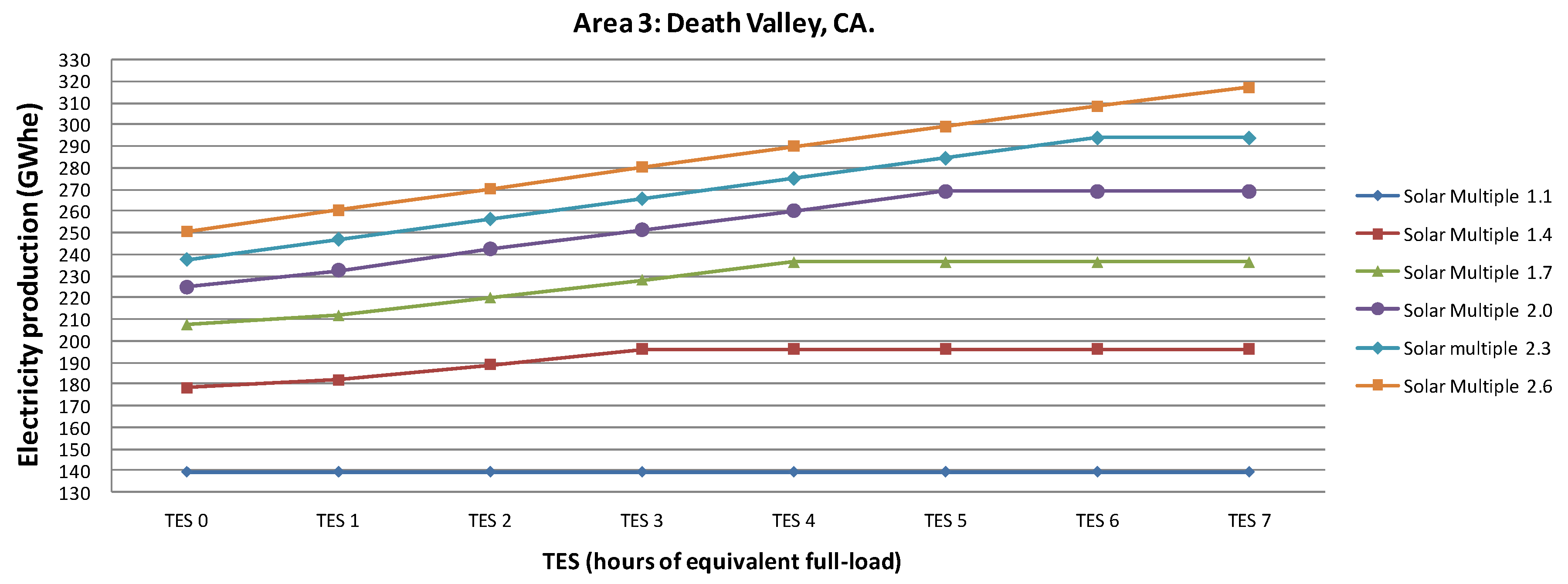
Death Valley, CA optimal TES (eq. hours)	0	1	3	3	4	5	6	7	7

summarizes the optimal sizing for TES and SM values, set according to their most profitable values from Figure 6, Figure 7 and Figure 8.

3.2. Technoeconomic Sensitivity Analysis

As shown in other works [14,15], economic analysis is focused on the LCOE. In (24), LCOE is used to compare the costs of electric-energy production according to the different plant configurations as a function of SM or TES:

$$LCOE=\frac{{{\displaystyle \sum }}_{t=1}^n(I_t+O\&M_t+F_t)}{{{\displaystyle \sum }}_{t=1}^n{E}_t},$$

(24)

The capital cost in year t is calculated in Equation (25):

$$I_t=crf·I_c.$$

(25)

The capital recovery factor is calculated according to Equation (26):

$$crf=\frac{i·{\left(1+i\right)}^n}{{\left(1+i\right)}^n-1}-k.$$

(26)

Considering a depreciation period of 25 years and a debt interest rate of 8.0%, the main data assumptions from

Table 7. Main data for PT power plant—levelized cost of electricity (LCOE) calculation [16].

Concept	Units	Value
Site cost	€/m2	13.33
Solar field investment	€/m2	213.52
HTF system	€/kWhth	210.95
Power-plant investment	€/kWe	643.20
Two molten-salt-tank TES investment	€/KWhth	52.74
Indirect investment cost and contingency surcharge	%	16.00
Fixed Operation and Maintenance (O and M) cost	€/kWe/year	45
Variable O and M cost	€/MWhe	3.50
Higher Heating Value (HHV) natural-gas fossil backup price	c€/kWh	2.87
Debt-interest rate	%	8.00
Annual insurance rate	%/year	0.50
Capital recovery factor	%	8.38
Plant lifetime	N	25

were used for the economic analysis [16].

Regarding the considered radiation scenarios, electricity production and LCOE evolution values with SM were studied. Comparison results are represented in Figure 9 for Vittoria, Figure 10 for Posadas, and Figure 11 for Death Valley, CA. In this analysis, TES sizing for each SM value was according to Table 6.

As shown in Figure 9, electricity production in Area 1 increased at the same time as SM and TES did, up to 223.08 GWh_e with SM = 2.6. However, the LCOE downtrend changed its tendency at SM = 1.8 and 209.92 k€/GWh_e as the critical point. With an optimal TES of 4, electricity generation over 181.64 GWh_e (SM = 1.8) was unable to balance the solar field, thermal-storage system, and Operation and Maintenance (O and M) investment. In Figure 10, an SM value of 2.0 was the most profitable solar-field size in order to obtain the maximum PT plant-investment optimization for Area 2. The best storage dimension of 5 equivalent hours for SM = 2.0 offered optimal electricity generation and LCOE values of 226.99 GWh_e and 182.08 k€/GWh_e, respectively. Regarding Figure 11, unless the electric generation uptrend rose to 317.60 GWh_e with SM = 2.6, values of SM above 2.2 carried an unprofitable tendency. At SM = 2.2, together with TES = 6, LCOE found its critical point. For this point, optimal plant sizing was set with a LCOE value of 155.35 k€/GWh_e and electricity production of 291.34 GWh_e.

3.3. Regulated- vs Deregulated-Electricity-Market Assesment

Optimal plant-design values were considered according to electrical production that minimizes LCOE, where generation best offsets plant investments. Economic results according to the most favorable LCOE values for each radiation scenario are represented in

Table 8. Economic results for a 100 MW_e PT power plant with two-tank molten-salt TES.

Location	Vittoria	Posadas	Death Valley, CA
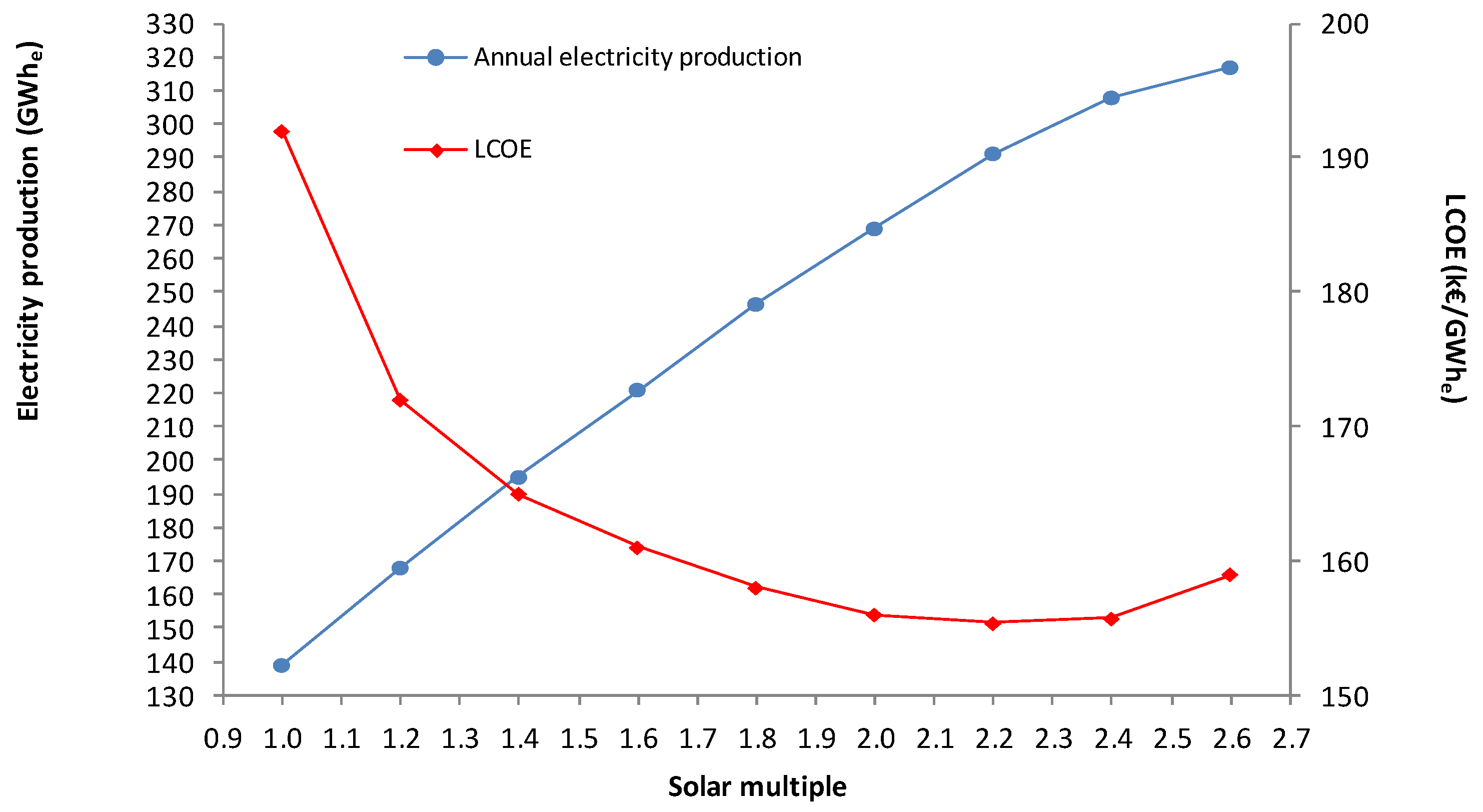
Solar-multiple value	1.8	2.0	2.2
Two-tank TES (equivalent hours)	4	5	6
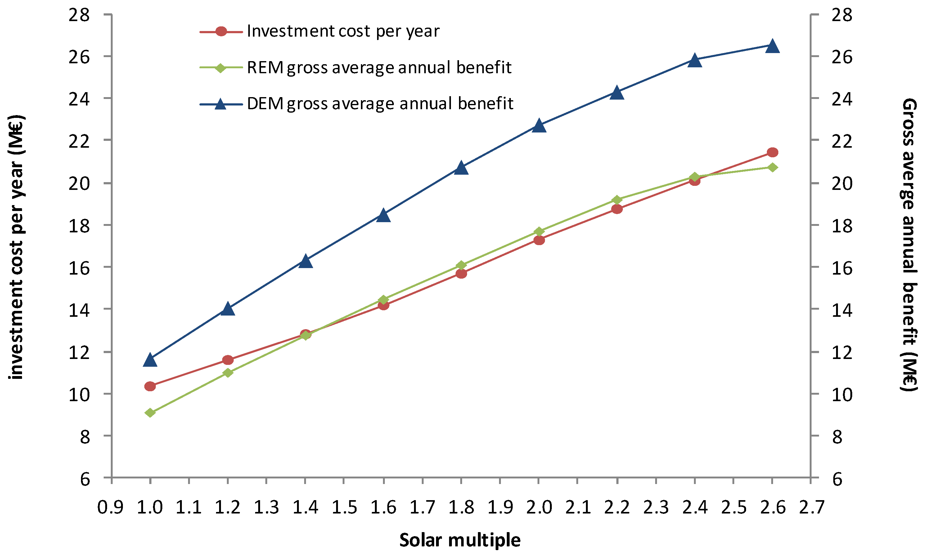
Total investment cost per year (M€)	15.49	17.14	18.77
Annual O and M cost (M€)	5.51	5.77	6.10
Annual fuel-consumption cost (M€)	0.046	0.051	0.057
Annual net electric-energy production (GWhe)	181.64	226.99	291.34
Capacity factor (%)	20.65	25.96	33.38
Annual LCOE (k€/GWhe)	209.92	182.08	155.82
REM gross average annual benefit (M€)	11.89	14.53	19.04
DEM gross average annual benefit (M€)	15.20	18.58	24.30

. REM and DEM gross average annual selling benefits were considered to set a comparison basic.

As shown in Table 8, optimizing the LCOE does not imply plant-investment viability. For REM, in Areas 1 (Vittoria) and 2 (Posadas), the gross average annual benefit did not exceed the total investment cost per year. Only for Area 3 (Death Valley, CA) did it have an annual gross profit that overcame the total cost of investment at 1.42%. Regarding DEM, Area 2 and 3 benefits exceeded the investment costs by 7.75% and 22.76%, respectively. However, benefits in low-radiation scenarios like Area 1 do not match the cost of the plant, posing a viability disadvantage (–1.91%).

Second analysis involves a plant configuration that allowed the highest electricity-sales profit versus investment cost. Figure 12, Figure 13 and Figure 14 show the total cost of investment per year and the average gross annual profit. Represented in Figure 12, Figure 13 and Figure 14 is the REM and DEM evolution with MS for each of the three radiation scenarios. TES sizing for each SM value is according to Table 6.

According to Figure 12, Figure 13 and Figure 14, plant sizing under REM found its optimal operation point at SM values of 1.8 for Vittoria, 2.0 for Posadas, and 2.2 for Death Valley. These values matched the results given in Table 8. For DEM, the most profitable plant operation in Area 1 (Vittoria) was made with SM = 2.0 and 4 TES equivalent hours, as shown in Figure 12. Nevertheless, gross average annual benefit (€16.70 M) did not rise above the annual investment cost (€16.89 M). Represented in Figure 13, an SM of 2.2 and TES of 6 was the best plant investment solution in Area 2 (Posadas). The benefits overcame plant investment costs by 8.07%. As plotted in Figure 14 for Area 3 (Death Valley), profit rose to €25.91 M with an SM of 2.4 and TES of 7. This is 22.77% over the annual investment cost of €20.01 M.

Table 9. Optimal economic results in a DEM for a 100 MW_e PT power plant with two-tank molten-salt TES.

Location	Vittoria	Posadas	Death Valley, CA
Solar-multiple value	2.0	2.2	2.4
Two-tanks TES (equivalent hours)	4	6	7
Total investment cost per year (M€)	16.89	18.46	20.01
Annual O and M cost (M€)	5.66	5.93	6.25
Annual fuel-consumption cost (M€)	0.051	0.057	0.062
Annual net electric-energy production (GWhe)	196.35	243.80	308.05
Capacity factor (%)	22.6	27.89	35.24
Annual LCOE (k€/GWhe)	210.31	183.13	157.28
DEM gross average annual benefit (M€)	16.70	20.08	25.91

summarizes the optimal DEM investment results for the three areas under study.

4. Discussion

The results obtained in this work for regulated markets, demonstrates that LCOE showed accurate analysis of the PT plant configuration. As shown in Figure 9, Figure 10 and Figure 11, when the LCOE changed its downward trend, it decreased cost-production margins, making it unviable. Optimal plant sizing regarding SM, and therefore TES, for an optimal LCOE matches each radiation scenario with benefits against investment costs, as from Figure 12, Figure 13 and Figure 14. In a deregulated market, electricity profit increment in high-priced periods makes optimal PT plant sizing tend to enhance SM and TES in any of the studied scenarios. Although LCOE moved from its best value, DEM improved average annual gross profit versus average annual total investment, as shown in Table 9.

Gross average annual benefit for electricity generation of deregulated against regulated markets was over 21% in all of the radiation areas under study. For medium- and high-radiation scenarios, DEM favors electricity sales profit to overcome investment costs for plant sustainability. Nevertheless, for low-radiation scenarios, benefits cannot offset investment costs, even in deregulated markets.

5. Conclusions

In this work, a 100 MW_e PT plant with a two-tank molten-salt TES was analyzed from an operation and market-behavior point of view. A mathematical simulation model was created and validated via a currently operated PT plant. Three locations representing different solar DNI scenarios were considered. Regulated and deregulated electricity-markets were considered for data analysis and investment optimization. Regarding solar resources and the electricity-markets, plant-sizing optimization was carried out according to [1.0:0.1:2.6] SM and [1:1:7] TES values.

Thus, the optimal dimensioning of a PT plant, considering as variables the size of the solar field and the thermal-storage capacity was shown in this paper, regarding the type of EM, for three different radiation scenarios. Based on this previous analysis, the electricity-production and LCOE evolution values with SM and TES were studied. In this technoeconomic analysis, the values of generated power that corresponded to an optimal value of LCOE, and therefore the optimal working points of the PT plant, were obtained. Finally, the optimal dimensioning values were parameterized in the operation of the PT plant under regulated and deregulated electricity-market requirements, obtaining the most profitable benefit results for each electricity-market scenario.

The main characteristic of the presented work was the great dimension-value vectors and the stochastic kind of values obtained depending on uncertain factors, such as weather forecast parameters. This study gives the best operation enouncement, and the obtained results allow for future- and historical-value analyses.

References

- Kearney, D.; Kelly, B.; Cable, R.; Potrovitza, N.; Herrmann, U.; Nava, P.; Mahoney, R.; Pacheco, J.; Blake, D.; Price, H. Overview on use of a molten salt HTF in a trough solar field. In Proceedings of the NREL: Parabolic Trough Thermal Energy Storage Workshop, Golden, CO, USA, 20–21 February 2003. [Google Scholar]
- Brogren, M. Optical Efficiency of Low-Concentrating Solar Energy Systems with Parabolic Reflectors. Ph.D. Thesis, Acta Universitatis Upsaliensis, Uppsala University, Uppsala, Sweden, 2004. [Google Scholar]
- Castronuovo, E. Optimization Advances in Electric Power Systems; Nova Science Publishers Inc.: New York, NY, USA, 2008; ISBN 978-1-60692-613-0. [Google Scholar]
- Union, E. Directive 2009/28/EC of the European Parliament and of the Council of 23 April 2009 on the promotion of the use of energy from renewable sources and amending and subsequently repealing Directives 2001/77/EC and 2003/30/EC. Off. J. Eur. Union 2009, 5, 2009. [Google Scholar]
- Bullejos, D.; Llamas, J.; De Adana, M.R. Spanish regulated scenarios for renewable energy and CSP plants. Arpn J. Eng. Appl. Sci. 2015, 10, 7217–7222. [Google Scholar]
- Oro, E.; Gil, A.; de Gracia, A.; Boer, D.; Cabeza, L.F. Comparative life cycle assessment of thermal energy storage systems for solar power plants. Renew. Energy 2012, 44, 166–173. [Google Scholar] [CrossRef]
- Bathurst, G.N.; Strbac, G. Value of combining energy storage and wind in short-term energy and balancing markets. Electr. Power Syst. Res. 2003, 67, 1–8. [Google Scholar] [CrossRef]
- Union, E. EU Energy in Figures. Statistical Pocketbook; Publication Office of the European Union: Brussels, Belgium, 2018; ISBN 978-92-79-88737-6. [Google Scholar] [CrossRef]
- Kumaresan, G.; Sridhar, R.; Velraj, R. Performance studies of a solar parabolic trough collector with a thermal energy storage system. Energy 2012, 47, 395–402. [Google Scholar] [CrossRef]
- Reddy, V.S.; Kaushik, S.C.; Tyagi, S.K. Exergetic analysis and performance evaluation of parabolic trough concentrating solar thermal power plant (PTCSTPP). Energy 2012, 39, 258–273. [Google Scholar] [CrossRef]
- Martin, L.; Mariano, M. Optimal year-round operation of a concentrated solar energy plant in the south of Europe. Appl. Eng. 2013, 59, 627–633. [Google Scholar] [CrossRef]
- El Hefni, B.; Soler, R. Dynamic multi-configuration model of a 145 MWe concentrated solar power plant with the ThermoSysPro library (tower receiver, molten salt storage and steam generator). Energy Procedia 2015, 69, 1249–1258. [Google Scholar] [CrossRef][Green Version]
- Garcia, L.I.; Alvarez, J.L.; Blanco, D. Performance model for parabolic trough solar thermal power plants with thermal storage: Comparison to operating plant data. Sol. Energy 2011, 85, 2443–2460. [Google Scholar] [CrossRef]
- Llamas, J.; Bullejos, D.; Ruiz de Adana, M. Techno-economic assessment of heat transfer fluid buffering for thermal ENERGY storage in the solar field of parabolic trough solar thermal power plants. Energies 2017, 10, 1123. [Google Scholar] [CrossRef]
- Abdul Baseer, M.; Awan, A.B.; Zubair, M. Performance analysis and optimization of a parabolic trough solar power plant in the middle east region. Energies 2018, 11, 741. [Google Scholar] [CrossRef]
- System Advisor Model Version 2017.9.5 (SAM 2017.9.5). National Renewable Energy Laboratory: Golden, CO, USA. Available online: https://sam.nrel.gov/content/downloads (accessed on 2 March 2019).
- Boukelia, T.E.; Mecibah, M.S.; Kumar, B.N.; Reddy, K.S. Optimization, selection and feasibility study of solar parabolic trough power plants for Algerian conditions. Energy Convers. Manag. 2015, 101, 450–459. [Google Scholar] [CrossRef]
- Poullikkas, A. Economic analysis of power generation from parabolic trough solar thermal plants for the Mediterranean region-a case study for the island of Cyprus. Renew. Sustain. Energy Rev. 2009, 13, 2474–2484. [Google Scholar] [CrossRef]
- Abbas, M.; Belgroun, Z.; Aburidah, H.; Merzouk, N.K. Assessment of a solar parabolic trough power plant for electricity generation under Mediterranean and arid climate conditions in Algeria. Energy Procedia 2013, 42, 93–102. [Google Scholar] [CrossRef]
- Reddy, K.S.; Kumar, K.R. Solar collector field design and viability analysis of standalone parabolic trough power plants for Indian conditions. Energy Sustain. Dev. 2012, 16, 456–470. [Google Scholar] [CrossRef]
- Bishoyi, D.; Sudhakar, K. Modeling and performance simulation of 100 MW PTC based solar thermal power plant in Udaipur India. Case Stud. Eng. 2017, 10, 216–226. [Google Scholar] [CrossRef]
- Shouman, E.R.; Khattab, N.M. Future economic of concentrating solar power (CSP) for electricity generation in Egypt. Renew. Sustain. Energy Rev. 2015, 41, 1119–1127. [Google Scholar] [CrossRef]
- Guédez, R.; Spelling, J.; Laumert, B. Thermoeconomic optimization of solar thermal power plants with storage in high-penetration renewable electricity markets. Energy Procedia 2014, 57, 541–550. [Google Scholar] [CrossRef][Green Version]
- Usaola, J. Operation of concentrating solar power plants with storage in spot electricity markets. IET Renew. Power Gener. 2012, 6, 59–66. [Google Scholar] [CrossRef]
- Casati, E.; Casella, F.; Colonna, P. Design of CSP plants with optimally operated thermal storage. Sol. Energy 2015, 116, 371–387. [Google Scholar] [CrossRef]
- Llamas, J.M.; Bullejos, D.; Ruiz de Adana, M. Optimal operation strategies into deregulated markets for 50 MWe parabolic trough solar thermal power plants with thermal storage. Energies 2019, 12, 935. [Google Scholar] [CrossRef]
- Sioshanshi, R.; Denholm, P. The Value of Concentrating Solar Power and Thermal Energy Storage; Technical Report NREL-TP-6A2-45833; National Renewable Energy Laboratory: Golden, CO, USA, 2010.
- International Energy Agency Technology Roadmap. Concentrating Solar Power. Available online: http://www.iea.org (accessed on 11 December 2018).
- Kazempour, J.; Moghaddam, P. Electric energy storage systems in a market-based economy: Comparison of emerging and traditional technologies. Renew. Energy 2009, 34, 2630–2639. [Google Scholar] [CrossRef]
- Martínez-Val, J.M. La Energía en sus Claves; Fundación Iberdrola: Madrid, Spain, 2004; ISBN 84-609-1337-6. [Google Scholar]
- XU, X.; Vignarooban, K.; Xu, B.; Hsu, K.; Kannan, A.M. Prospects and problems of concentrating solar power technologies for power generation in the desert regions. Renew. Sustain. Energy Rev. 2016, 53, 1106–1131. [Google Scholar] [CrossRef]
- Habib, L.; Hassan, M.I.; Shatilla, Y. A realistic numerical model of lengthy solar thermal receivers used in parabolic trough CSP plants. Energy Procedia 2015, 75, 473–478. [Google Scholar] [CrossRef]
- Dunn, R.I.; Hearps, P.J.; Wright, M.N. Molten-salt power towers: Newly commercial concentrating solar storage. Proc. IEEE 2012, 504–515. [Google Scholar] [CrossRef]
- Cervantes, R.; Quéméré, G.; Luque-Heredia, I. Sunspear calibration against array power output for tracking accuracy monitoring in solar concentrators. In Proceedings of the European Photovoltaic Solar Energy Conference, Valencia, Spain, 1–5 September 2008; pp. 890–893. [Google Scholar]
- Almasabi, A.; Alobaidli, A.; Zhang, T.J. Transient characterization of multiple parabolic trough collector loops in a 100 MW CSP plant for solar energy harvesting. Energy Procedia 2015, 69, 24–33. [Google Scholar] [CrossRef]
- Centro de Investigaciones Medioambientales, energéticas y tecnológicas (CIEMAT), Prospectiva y vigilancia tecnológica de energía solar térmica de concentración. Available online: http://www.ciemat.es (accessed on 5 September 2018).
- National Aeronautics and Space Administration (NASA). Prediction of Worldwide Resources. Available online: https://power.larc.nasa.gov/ (accessed on 11 June 2019).
- Turchi, C. Parabolic trough Reference Plant for COST Modeling with the Solar Advisor Model; Technical Report NREL/TP-550-47605; National Renewable Energy Laboratory (NREL): Golden, CO USA, 2010.
- Reddy, R.G.; Wu, B.; Rogers, R. Ionic Liquids as Thermal Energy Storage Media for Solar Thermal Electric Power Systems; University of Alabama: Tuscaloosa, AL, USA, 2001; Available online: https://p2infohouse.org/ref/22/21020.pdf (accessed on 8 May 2018).
- Desai, N.; Bandyopadhyay, S. Optimization of concentrating solar thermal power plant based on parabolic trough collector. J. Clean. Prod. 2015, 89, 262–271. [Google Scholar] [CrossRef]
- Teske, S. Concentrated Solar Thermal Power. Available online: https://www.greenpeace.de/sites/www.greenpeace.de/files/greenpeace_studie_solar_thermal_power_englisch_1.pdf/ (accessed on 16 February 2019).
- Eutech Scientific Engineering. Thermolib User Manual. Available online: https://www.thermolib.de/media/thermolib/downloads/Thermolib-UserManual.pdf (accessed on 24 August 2015).
- Mathworks. The Mathwork, SymPowerSystems 5. Available online: http://www.mathworks.com. (accessed on 28 February 2019).