Influences of Optical Factors on the Performance of the Solar Furnace

Abstract

In this paper, an optical structure design for a solar furnace is described. Based on this configuration, Monte Carlo ray tracing simulations are carried out to analyze the influences of four optical factors on the concentrated solar heat flux distribution. According to the practical mirror shape adjustment approach, the curved surface of concentrator facet is obtained by using the finite element method. Due to the faceted reflector structure, the gaps between the adjacent mirror arrays and the orientations of facets are also considered in the simulation model. It gives the allowable error ranges or restrictions corresponding to the optical factors which individually effect the system in Beijing: The tilt error of heliostat should be less than 4 mrad; the tilt error of the concentrator in the orthogonal directions should be both less than 2 mrad; the concentrator facets with the shape most approaching paraboloid would greatly resolve slope error and layout errors arising in the concentrator. Besides, by comparing the experimentally measured irradiance with the simulated results, the optical performance of the facility is evaluated to investigate their comprehensive influence. The results are useful to help constructors have a better understanding of the solar furnace’s optical behavior under conditions of multiple manufacture restrictions.

1. Introduction

In solar thermal power applications, the solar furnace has globally served as an ideal test-bed to develop key technologies required for high temperatures (up to 3500 K), and thus is used for its capability of concentrating solar radiation to factors of more than thousands of suns [1]. Solar furnaces are used for the investigation of high-temperature action on materials and equipment in many fields, such as thermochemistry [2] and hydrogen production [3]. During more than half of a century evolvement, largescale solar furnaces and solar furnaces with various optical structure designs have been constructed to allow for experiments in various fields such as thermochemistry. In Odeillo, France, the CNRS has been operating a 1000 kW thermal power solar furnace since 1968. It is known as one of the biggest solar furnaces in the world, consisting of 63 heliostats and a parabolic concentrator with an 1830 m² aperture area [4]. There is another facility with the same capacity that was commissioned in 1987 in Parkent, Uzbekistan [5]. The solar furnace in PSA [6], named SF40, has a similar optical structure design to the one in KIER [7]. They are composed of a flat heliostat with a no-concentration effect and a revolution paraboloid dish, and achieve very high concentrated solar heat flux and thermal gradients. Zhang et al. [8] proposed a line-focused solar concentrating system to extend the possible experimental support. The shape of the mirror arrays, also called facets, are chosen to be hexagonal for good fill in the concentrator area for the solar furnace in Mexico [9]. In addition, the solar furnace in DLR [10] takes the advantage of an off-axis solution to efficiently avoid the shadow from objects installed in the focal region onto the concentrator.

Typically, solar furnaces of the small and medium sizes usually adopt two sets of mirror devices, with one being a heliostat and one being a concentrator. As the decisive component responsible for concentrating sunlight, the concentrator’s optical characteristics directly determine the operating performance of the solar furnace [6]. Despite a continuous support for the revolution paraboloid as the ideal design for the concentrator, the considerable cost in its manufacture and its time-consuming testing are crucial impediments for its commercial application, in addition to its extremely high demands in precision. Thus, a practical and economical alternative using a faceted structure covered with identical curved mirror arrays is more common practice. The study [11] has concluded that point-focused collectors have an acceptable performance that strongly depends on facet sizes and optical errors, although the final result differs from that of an equivalent ideal paraboloid. However, its optical characteristics in the solar furnace remain unknown in regards to the faceted concentrator receiving sunlight from the heliostat instead of the sun. Besides, there are few studies on how other optical factors effect the working performance of the solar furnace. In terms of an ideal high-temperature solar thermal facility capable of a reaching a substantial market, this study seeks to figure out the individual and coupling impacts of basic optical factors on this specific concentrating system, thereby providing better guidance in fabrication and assembling to achieve the optimal working conditions.

Concentrated solar heat flux distribution provides a basic measure to evaluate the optical performance of a concentrating system, including the peak heat flux and the spot size. Its value represents the highest attainable concentrated solar irradiance for a blackbody. In general, concentrated heat flux can be measured experimentally, which relies on numbers of precise and fast responsive microsensors [12]. Additionally, it can also be estimated by means of simulation. The Monte Carlo ray tracing (MCRT) method is very flexible and has been proved to have a great accuracy: Li et al. performed the MCRT simulation on a Xe-arc lamp, with results of radiation power 0.32% higher than the experiment measurement [13]; Zhao et al. set up the MCRT model for the parabolic trough collector, and it had good agreement with the theoretical formula [14]. Additionally, the MCRT method is effectively used to design and optimize the parameters for a solar concentrating system [15,16]. The principle of the MCRT is as follows: A large amount of solar rays’ behavior in a mirror field such as reflection, intersection and escape are traced, and the final concentrated heat flux distribution is derived by statistically counting the number of rays reaching the surface of the focusing target. Moreover, if the representative variables that account for influencing factors are considered in the model, by the MCRT simulations, it equally allows an assessment of the concentration accuracy of the concentrating system [7]. Basically, factors mainly influencing the final concentrated heat flux distribution can be grouped in to two major categories: Optical errors and geometrical errors [17]. Among them, factors such as specular reflectance errors [18,19] and tracking errors [20] can now be controlled well in comparatively ideal conditions, due to the increasingly sophisticated knowledge and technology available. As a result, the optical factors which directly effect the reflective surface normal vector have become the main sources deteriorating the optical performance of the concentrating system. Their existence would even double the offset in sunlight reflection. Therefore, here in this work, the approach of adding error models in MCRT is chosen to evaluate the performance of the solar furnace and analyze influences of optical factors.

In this paper, an optical structure of the solar furnace is described. The solar furnace with this design, chosen as the study case, was constructed in the solar thermal power plant in Yanqing, Beijing [21,22]. Four types of optical factors that impact on the concentrated heat flux distribution are analyzed by MCRT simulations: The tilt error of the heliostat, which originates from heliostat facets deviating from the ideal plane; the slope error of the concentrator, referring to the irregular deformation of reflecting curves of the concentrator facets by the surface adjustment approach; the layout error of the concentrator, caused by the same or similar shape of facets attached to the concentrator frame; and the tilt error of the concentrator, which arises from concentrator facets tilting. All of them strongly effect on the sunlight path in mirror field of the solar furnace optical system. In particular, results differ from the available references which take the integral concentrator mirror surface or facets of it as an idealized paraboloidal, whereas here we have adopted the finite element method (FEM) to better represent the practical reflecting surface. A high-order linear fitting curve synthesizes the concentrator facet surface by fitting discrete points obtained from the FEM. The constraints are the displacements of adjusting bolts in the rear of mirror arrays and position the connecting pad located. The validated MCRT model is mixed-programed in C++ and MATLAB. By analyzing the simulation results, the study gives the allowable error ranges when each factor effects individually. In the final part, comparisons between the results from simulations and the results obtained by experimental measures provide comprehensive influences of four factors, and indicate some possible causes leading to the differences.

2. Structure Design

On-axis configuration is applied in present case, for the consideration of minimizing the axis aberration effect. The main components of the optical system and receiver are placed on the same line, joining the center of the concentrator and the center of the heliostat. Due to the relatively high latitude of Beijing, it is decided to use a north-south arrangement, that locates the heliostat north of the concentrator and with the receiver placed at the focal area. As shown in Figure 1, the working principle is as follows: The heliostat uses a two-axis tracking strategy to track the sun and reflects solar rays horizontally and in parallel to the optical global axis of the concentrator. The concentrator concentrates incoming rays from the heliostat onto its focus. The receiving surface placed with testing material or equipment is eventually irradiated with a highly-concentrated solar radiation.

The heliostat consists of flat reflective facets and rotating arms. It differs from those in the concentrating solar power plant, as the heliostat in the solar furnace has no concentration effect. Reflected rays from the heliostat are constantly kept in the expected direction, horizontal and parallel to the concentrator’s optical axis. All facets are attached to the plane frame of the heliostat with connecting pieces. Also, they are aligned tightly in two perpendicular directions. Narrow gaps between adjacent facets are required for the leveling process. In addition, the two-axis rotating motion is continuously driven by an azimuth-evaluation tracking strategy in the computer with the PLC module.

The concentrator is the key component of the solar furnace. It is kept stationary on the ground to concentrate the sunlight onto the static position. Basically, it is the first priority to find the balance between the optical performance of the solar furnace and the cost primarily originated from the concentrator. Thus, it is the common practice to use the faceted structure covered with identical approximate paraboloid facets. Before being installed to the supporting frame, each facet’s center is fixed to its bracket by a connecting pad, contacted with a finite number of adjusting bolts (eight in this paper) in the rear. By the method of regulating the lengths of the adjusting bolts, the flat mirror can be deformed to a desired curved surface which meets the requirement. Those facets with similar curvature are subsequently attached to the concentrator frame with an individual optical axis which is normal to their respective positions. Certainly, in such way, it may reduce the performance in concentrating solar power to some extent. However, in return, this approach greatly lowers the price and difficulty in fabrication and shortens the commissioning time. Besides, the focusing effect in the optimal conditions is totally acceptable compared with the ideal situation, which will be fully discussed in the following sections. As similar to the heliostat, facets of the concentrator must be carefully aligned. In addition, the receiver platform is placed between two mirror devices at the focal point of the concentrator. In this way, the entrance area could be exposed to the highest attainable solar irradiance.

3. Methods

For using the MCRT method, the mirror field is first set up based on working conditions of the concentrating system, including the physical placement of the main mirror devices, and orientation of the reflecting surface. According to the working principle of the solar furnace, the solar power concentrating process is divided into four parts: The solar position tracking, primary reflection by the heliostat, secondary concentration by the concentrator, and heat flux calculation on the receiver surface. Figure 1 shows five right-handed cartesian systems adopted in modelling. They are, respectively, the ground co-ordinate system $O_G$, heliostat co-ordinate system $O_H$, concentrator co-ordinate system $O_C$, concentrator facet co-ordinate system $O_{c_j}$ and receiver co-ordinate system $O_R$. Here, the methodology is based on the following assumptions:

• Incidence sunlight is treated as an optic cone.
• Heliostat facets are perfect flat surfaces.
• Concentrator facets are perfect curved surfaces.
• The center of the facets on the faceted concentrator is located at the point on a continuous revolution paraboloid with the equivalent focal distance.
• All traced solar rays have equal solar energy regardless of the angles of incidence.

3.1. Sun Position Tracking

To achieve the tracking strategy, it requires to acquire the sun position before determining heliostat’s rotating motion. Here, classical simplified equations of the sun position are used [23], in $O_G$:

$$\begin{array}{l}{\alpha }_s=\mathrm{asin}\left(\sin \varphi \sin \delta +\cos \varphi \cos \delta \cos \omega \right)\\ {\gamma }_s=\frac{3\pi }{2}-\mathrm{sign}\omega \left|\mathrm{acos}\left(\frac{\sin {\alpha }_{sun}\sin \varphi -\sin \delta }{\cos {\alpha }_{sun}\cos \delta }\right)\right|\end{array}$$

(1)

where ${\alpha }_s$ is the solar altitude angle, positive above the horizontal plane; ${\gamma }_s$ is the solar azimuth angle, positive counterclockwise from the east; $\varphi$ is the local latitude; $\delta$ is the declination; $\omega$ is the hour angle. The latter three variables can be solved, as in the reference [23]. Note that, in this paper, the Greek letter $\alpha$ refers to the altitude angle of a vector, and the letter $\gamma$ refers to the azimuth angle.

The heliostat adopts an azimuth-elevation biaxial tracking strategy. The first rotating axis is perpendicular to the ground, and the heliostat rotates along this axis with value ${\gamma }_H$, defined as the azimuth angle of the heliostat’s global axis. The second axis is parallel to the ground and perpendicular to the first axis, and the heliostat does rotation along this axis with value ${\alpha }_H$, defined as the altitude angle of the heliostat’s global axis. Both of two terms determine the tracking state of the heliostat and make sure the incoming rays from the sun can be reflected in the expected direction on the concentrator.

In $O_G$, the solar incidence optic cone center vector $\overrightarrow{s_s}$ and the primary reflected optic cone center $\overrightarrow{t_s}$ are given as Equation (2). $\overrightarrow{s_s}$ can be derived from Equation (1) and the azimuth angle and altitude angle in $\overrightarrow{t_s}$, respectively ${\gamma }_{h2t}$ and ${\alpha }_{h2t}$, are known from the relative position between the center of the integral heliostat mirror surface and the tracking target on the concentrator. Normally, in on-axis configuration, the tracking point is the center of the integral concentrator mirror surface if there is no geographic height difference between the two devices. On the basis of the law of reflection, it is easy to get the values of ${\gamma }_H$ and ${\alpha }_H$ by solving Equation (3), where $\overrightarrow{n_H}$ is the unit vector of the heliostat global optical axis, and ${\theta }_s$ is the solar incidence angle. Noted that $R_s$ is the solar rotation matrix and all the matrixes concerning rotation and coordinate transformation are listed in the Appendix A.

$$\begin{array}{l}\overrightarrow{s_s}=\left[0,0,1\right]R_s=\left[\cos {\alpha }_s\cos {\gamma }_s,\cos {\alpha }_s\sin {\gamma }_s,\sin {\alpha }_s\right]\\ \overrightarrow{t_s}=\left[\cos {\alpha }_{h2t}\cos {\gamma }_{h2t},\cos {\alpha }_{h2t}\sin {\gamma }_{h2t},\sin {\alpha }_{h2t}\right]\end{array}$$

(2)

$$\begin{array}{l}\overrightarrow{s_s}+\overrightarrow{t_s}=2\cdot \overrightarrow{n_H}\cdot \cos {\theta }_s\\ \cos 2{\theta }_s=\overrightarrow{s_s}\cdot \overrightarrow{t_s}\\ \overrightarrow{n_H}=\left[\cos {\alpha }_H\cos {\gamma }_H,\cos {\alpha }_H\sin {\gamma }_H,\sin {\alpha }_H\right]\end{array}$$

(3)

3.2. Optical System Models

In co-ordinate $O_H$, a random solar incidence ray is represented as Equation (4). The radial angle $\phi$ and circumferential angle $\psi$ for a random solar ray are expressed as Equation (5) [14]:

$$\overrightarrow{s_1}=-\left[\sin \phi \cos \psi ,\sin \phi \sin \psi ,\cos \phi \right]\cdot R_s\cdot M_{G2H}$$

(4)

$$\begin{array}{l}\phi =\mathrm{atan}\left(\sqrt{{\epsilon }_1}\tan {\phi }_{\max }\right)\\ \psi =2\pi {\epsilon }_2\end{array}$$

(5)

where $M_{G2H}$ is co-ordinate transform matrix from $O_G$ to $O_H$, ${\epsilon }_1$ and ${\epsilon }_2$ are random numbers between 0 and 1, ${\phi }_{\max }$ represents the radial angle of the incident solar optic cone.

To set up a mirror field, it starts with the heliostat optical model. The integral heliostat surface is segmented into many pieces of flat mirrors. It is necessary to number facets to find which one of them intersects with and reflects the random solar ray. When considering error models of the heliostat, the error resulted from facets rotating in the heliostat mirror plane is neglected, due to the confinement of very narrow gaps between the adjacent facets. Furthermore, engineering measures can now better control a facet’s vertical offset, within a few millimeters. Its impact on the final result is minuscule, thus, which is also neglected. Based on assumption 2, the optical model for the heliostat can be further simplified. Here, it is assumed that a heliostat facet is kept in the ideal position and only the local optical axis is deflected because of facet’s tilting. The area changes in the integral sunlight receiving surface is the sum of the cosine values of facets between the local optical axis and the ideal surface normal vector (which is parallel to the z-axis of $O_H$). As illustrated in Figure 2, the local optical axis with tilting error of the i-th heliostat facet $\overrightarrow{n_{h_{{}_i}}}$ is expressed as Equation (6). The area changes in the integral sunlight receiving surface of the heliostat, ${\eta }_1$, is given as Equation (7).

$$\begin{array}{cc}\begin{array}{ll}\overrightarrow{n_{h_{{}_i}}}\hfill & =\overrightarrow{n_H}\cdot M_{G2H}\cdot E_{h_i}=\left[0,0,1\right]\cdot E_{h_i}\hfill \\ & =\left[\sin {\phi }_{h_i}\cos {\psi }_{h_i},\sin {\phi }_{h_i}\sin {\psi }_{h_i},\cos {\phi }_{h_i}\right]\hfill \end{array}& i=1,2,\dots ,r_h\cdot c_h\end{array}$$

(6)

$${\eta }_1=\frac{{\displaystyle {\sum }_{i=1}^{r_h\cdot c_h}\overrightarrow{n_{h_i}}\cdot \left(\overrightarrow{n_H}\cdot M_{G2H}\right)\cdot S_{h_i}}}{{\displaystyle {\sum }_{i=1}^{r_h\cdot c_h}{S}_{h_i}}}=\frac{{\displaystyle {\sum }_{i=1}^{r_h\cdot c_h}\overrightarrow{n_{h_i}}\left(z\right)\cdot S_{h_i}}}{S_H}$$

(7)

where the radial angle ${\phi }_{h_i}$ and circumferential angle ${\psi }_{h_i}$ introduced into the ideal normal vector represent the i-th heliostat facet tilting error; $r_h$ and $c_h$ are the row and column number of heliostat facets; $E_{h_i}$ is defined as the i-th heliostat facet’s tilting error matrix; $S_{h_i}$ is the area of the i-th facet; and $S_H$ is the neat area of the heliostat.

Based on the heliostat optical model described above, the primary reflection modeling is as follows: A random solar incidence ray $\overrightarrow{s_1}$ intersects with the i-th facet of the heliostat on point $P_1\left(x_{p_1},y_{p_1},z_{p_1}\right)$ where the local optical axis is $\overrightarrow{n_{h_i}}$, then the primary reflected ray $\overrightarrow{t_1}$ can be solved as Equation (8), where $H_{h_i}$ is the reflection matrix of the i-th heliostat facet.

$$\overrightarrow{t_1}=\overrightarrow{s_1}\cdot H_{h_i}=\overrightarrow{s_1}\cdot \left(\overrightarrow{e}\left(3\right)-2\cdot {\overrightarrow{n_{h_i}}}^T\cdot \overrightarrow{n_{h_i}}\right)$$

(8)

Similarly, the integral concentrator concentrating surface is faceted, and also the gaps between the mirrors are considered and facets are numbered when modeling. According to the aforementioned surface adjustment approach, the chosen structure with eight adjusting bolts and one connecting pad is shown as Figure 3. By this approach, the facet is deformed to a non-ideal complex curved surface, which causes the slope error. It could not be expressed with a simple formula. Thus, the FEM is applied to first obtain discrete points on the facet with the constraints of displacements of adjusting bolts and the fixed position of connecting pad. The fourth-order polynomial fitting is then used to obtain the facet equation for a higher fitting accuracy. All facets attached to the concentrator share the same curved surface equation under the same constraints. Take the j-th concentrator facet as an example, in $O_{c_j}$, its surface equation is expressed as Equation (9):

$$\begin{array}{cc}z=f_{c_j}\left(x^{\left(4\right)},y^{\left(4\right)}\right)& j=1,2,\dots ,r_c\cdot c_c\end{array}$$

(9)

where $r_c$ and $c_c$ are the row and column number of concentrator facets, respectively.

The tilting error of concentrator should be added in three dimensions, that involves the rotating around the $x_{c_j}$, $y_{c_j}$, and $z_{c_j}$ axis as illustrated in Figure 4. Considering the less than tens of millimeters gap size between facets, the rotation around the z-axis is neglected here. The rest of them take major parts in the deviation of the surface normal vector of each reflected point from its ideal direction. It is defined as the tilting error matrix of the j-th concentrator facet as $E_{c_j}$, in which the rotating angle around the positive direction of $x_{c_j}$ is ${\phi }_{c_j}$, and that of $y_{c_j}$ is ${\psi }_{c_j}$.

Moreover, by the same surface adjustment method, mirror arrays with the same or similar curvature cover the revolution paraboloid concentrator frame, which inevitably reduces off the concentrating performance, here defined as layout error. Facets placed on the respective positions have their own individual local optical axis normal to their center. Based on assumption 4, in $O_C$, the ideal paraboloid where facets center locate is given as Equation (10) with a focal length $F$. The azimuth and altitude angles of the global optical axis are ${\gamma }_C$ and ${\alpha }_C$, respectively, obtained from the concentrator’s stationary orientation. With those two variables, the co-ordinate transform matrix $M_{G2C}$ can be calculated. The j-th facet’s optical axis is as Equation (11). The x-axis rotation angle ${\gamma }_{c_j}$ and y-axis rotation angle ${\alpha }_{c_j}$ in the transform matrix $M_{C2c_j}$ are calculated as Equation (12).

$$f_{ce{n}_j}\left(x,y,z\right)=x^2+y^2-4Fz$$

(10)

$$n_{ce{n}_j}=\frac{-\left[\frac{\partial f_{ce{n}_j}}{\partial x},\frac{\partial f_{ce{n}_j}}{\partial y},\frac{\partial f_{ce{n}_j}}{\partial z}\right]}{{\left[\frac{\partial f_{ce{n}_j}}{\partial x},\frac{\partial f_{ce{n}_j}}{\partial y},\frac{\partial f_{ce{n}_j}}{\partial z}\right]}_2}$$

(11)

$$\begin{array}{l}{\gamma }_{c_j}=\mathrm{atan}\left(n_{ce{n}_j}\left(x\right)/n_{ce{n}_j}\left(z\right)\right)\\ {\alpha }_{c_j}=-\mathrm{asin}\left(n_{ce{n}_j}\left(y\right)\right)\end{array}$$

(12)

To sum up, the concentrator secondary concentration modeling is as follows: In $O_C$, an incidence ray $\overrightarrow{s_2}$ from the point $P_1^{\prime }$ on the heliostat intersects with the j-th concentrator facet on point $P_2^{\prime }$. The point $P_2^{\prime }$ is derived from the point $P_2\left(x_{p_2},y_{p_2},z_{p_2}\right)$ in $O_{c_j}$ by co-ordinates conversion between co-ordinate systems. As knowing $\overrightarrow{s_2}$ and the normal vector ${\overrightarrow{n_{c_j}}|}_{P_2^{\prime }}$ given as Equation (14) on $P_2^{\prime }$, the secondary reflected ray $\overrightarrow{t_2}$ then can be solved from Equation (15). Here, $H_{c_j}$ is the reflection matrix of the j-th concentrator facet. In $O_G$, $T_{G2H}=\overrightarrow{O_G{O}_H}$, $T_{G2C}=\overrightarrow{O_G{O}_C}$.

$$\begin{array}{l}\overrightarrow{s_2}=\overrightarrow{t_1}\cdot M_{G2H}^{-1}\cdot M_{G2C}\\ P_1^{\prime }=\left(P_1\cdot M_{G2H}^{-1}+T_{G2H}-T_{G2C}\right)\cdot M_{G2C}\\ P_2^{\prime }=P_2\cdot M_{C2c_j}^{-1}+[x_{ce{n}_j},y_{ce{n}_j},z_{ce{n}_j}]\end{array}$$

(13)

$${\overrightarrow{n_{c_j}}|}_{P_2^{\prime }}=\frac{\left[-\frac{\partial f_{c_j}}{\partial x_{p_2}},-\frac{\partial f_{c_j}}{\partial y_{p_2}},1\right]}{{\Vert \left[-\frac{\partial f_{c_j}}{\partial x_{p_2}},-\frac{\partial f_{c_j}}{\partial y_{p_2}},1\right]\Vert }_2}\cdot E_{c_j}^{-1}\cdot M_{C2c_j}^{-1}$$

(14)

$$\overrightarrow{t_2}=\overrightarrow{s_2}\cdot {H_{c_j}|}_{P_2^{\prime }}=\overrightarrow{s_2}\cdot \left(\overrightarrow{e}\left(3\right)-2\cdot {\overrightarrow{n_{c_j}}|}_{P_2^{\prime }}{}^T\cdot {\overrightarrow{n_{c_j}}|}_{P_2^{\prime }}\right)$$

(15)

3.3. Heat Flux Calculation

The solar furnace mainly uses the direct normal irradiance (DNI), and Equation (22) is adopted for the simulated value because it is suitable for the conditions in Beijing [24]:

$$\mathrm{DNI}=\frac{1376\left(1+0.033\cos \frac{2\pi n}{365}\sin {\alpha }_s\right)}{\sin a_s+{\eta }_a}$$

(16)

where $n$ is the date order, and in sunny day ${\eta }_a=0.33$.

The azimuth angle ${\gamma }_R$ and the altitude angle ${\alpha }_R$ of the global axis of the receiver surface can be known from its settled orientation, which is as same as the concentrator. Furthermore, the co-ordinate transform matrix $M_{G2R}$ is derived on the basis of those two variables. In $O_R$, given the secodary reflected ray $\overrightarrow{s_3}$, incidence ray from point $P_2^{″}$ on the concentrator, the intersection point with the receiver surface can be solved. Based on the MCRT method, incidence solar rays with the number of $N_t$ are traced and every single ray repeats the concentration procedure described above. To obtain the final concentrated heat flux distribution, the receiver surface is meshed into small rectangular area with the number of $r_r\cdot c_r$. The result is calculated as Equation (19).

$$\overrightarrow{s_3}=\overrightarrow{t_2}\cdot M_{G2C}^{-1}\cdot M_{G2R}$$

(17)

$$P_2^{″}=\left(P_2^{\prime }\cdot M_{G2C}^{-1}+T_{G2C}-T_{G2R}\right)\cdot M_{G2R}$$

(18)

$$\begin{array}{cc}{I}_k=\frac{N_k\cdot I_0}{S_k}=\frac{N_k}{S_k}\cdot \frac{\mathrm{DNI}\cdot S_H\cdot {\eta }_1\cdot {\eta }_2\cdot {\eta }_3\cdot {\eta }_4\cdot {\eta }_5}{N_t}& k=1,2,\dots ,r_r\cdot c_r\end{array}$$

(19)

where $I_k$ is the heat flux of the k-th mesh; $N_k$ is the number of rays fall in the k-th mesh; $S_k$ is the k-th mesh area; $I_0$ is the solar energy of one traced ray; ${\eta }_2$ is the cosine efficiency; ${\eta }_3$ is the reflectivity of heliostat; ${\eta }_4$ is the reflectivity of concentrator; and ${\eta }_5$ represents the degree of shading area.

4. Results and Discussion

4.1. Validation for the MCRT Model

The MCRT codes are programmed in mixed programing languages, which should be validated before the further study. This MCRT model is validated against the results available in the reference [11]. The parameters used for validation are summarized in

Table 1. Parameters used in the validation [11].

Name	Values
${\phi }_{\max }$ (mrad)	4.7
Heliostat (m × m)	12 × 10
Radius of the Circular of the Paraboloid Concentrator (m)	4
Focal Length (m)	15.512
DNI (W/m2)	970
${\eta }_3$	0.9
${\eta }_4$	0.9

and the comparisons are presented in Figure 5.

Generally, the accuracy of the MCRT method strongly depends on the numbers of tracing rays. Here, the number of 1 × 10⁸ rays are chosen. Besides, the distribution of the final concentrated heat flux is related to the both mesh size on the receiver surface and the solar model [25]. In the validation, it is decided to use square meshes of 10 × 10 mm for reducing computing time on heat flux calculation, and the same uniform distribution solar model as in the reference. From the Figure 5b, it agrees well with results in the available reference, which can verify the accuracy of the MCRT model used in the current paper.

Since it has to take the local fabrication capability into consideration, the practical parameters of the solar furnace in Yanqing, Beijing are listed in

Table 2. Parameters of the solar furnace in Yanqing, Beijing.

Name	Size (m × m)	Row & Column	Gap (mm)	Focal Length (m)
Heliostat	6.250 × 5.975	7 × 6	30	3.8
Concentrator	4.572 × 4.572 (Aperture)	15 × 15	10

, and the main components are presented as Figure 6. In the following cases analyzing optical factors influence, it adopts 12:00 PM on 21st March as the time, and Yanqing district in the north of Beijing (40.3833 N, 115.9367 E) as the location for the simulations, DNI 958 W/m², sun position ${\gamma }_s=4.66\mathrm{rad}$, ${\alpha }_s=0.86\mathrm{rad}$, radial angle ${\phi }_{\max }=4.65\mathrm{mrad}$, and the reflectivity of heliostat and concentrator are both set as 0.8.

To discern each optical factor effect, the simulations in the following four sections are based on an ideal reference solution of the solar furnace: The mirror arrays of the heliostat are perfectly flat and fixed on the same plane, and the facets of the concentrator are the perfect paraboloid curved with the focal of 3.8 m, and the local optical axis of each mirror units are oriented to the ideal direction normal to their respective positions.

4.2. Tilt Error of the Heliostat

Once facets are attached to the frame structure, their respective tilting angles are fixed. However, it is impossible to install or assemble the facets facing to the exactly ideal direction in an engineering practice, which also means the tilt error of facets has great randomness and uncertainty. To better represent the tilt error in the heliostat model, parameters ${\phi }_{h_i}$ and ${\psi }_{h_i}$ of facet tilt error are given by Equation (20), which is borrowed from the solar model representing uniform randomness.

$$\begin{array}{l}{\phi }_{h_i}=\mathrm{atan}\left(\sqrt{{\epsilon }_3}\tan {\phi }_{h\max }\right)\\ {\psi }_{h_i}=2\pi {\epsilon }_4\end{array}$$

(20)

where ${\epsilon }_3$ and ${\epsilon }_4$ are random numbers between 0 and 1, with the tilt error range of heliostat defined as $e_h=2\cdot {\phi }_{h\max }$.

Figure 7 shows how the center concentrated heat flux distribution varies with $e_h$. As is expected, the concentrated solar irradiance is irregularly scattering around as the error increases. Apparently, the error of the facets tilting away from ideal position deviates the local optical axis of the mirror pieces. In consequence, reflected rays from heliostat are no longer parallel to the global optical axis of concentrator. From the simulation cases, it can be seen that: When $e_h\le 8\mathrm{mrad}$, the heat flux distribution still maintains a good-shape Gaussian distribution, in particular, when $e_h=8\mathrm{mrad}$, the peak heat flux decreases to 84.3% of that in ideal case; when $e_h=4\mathrm{mrad}$, the heat flux distribution almost coincides with that in ideal conditions; as $e_h\ge 12\mathrm{mrad}$, the divergence of the concentrated solar power are serious, which means the optical performance of the solar furnace drops sharply. Nonetheless, even in the worst situation where facets tilt error is intolerable, the change in the sunlight receiving area of the heliostat is very small, specifically: ${\eta }_1=0.999975$, as $e_h=24\mathrm{mrad}$, which provides a reference for further simplifying the heliostat model in the solar furnace.

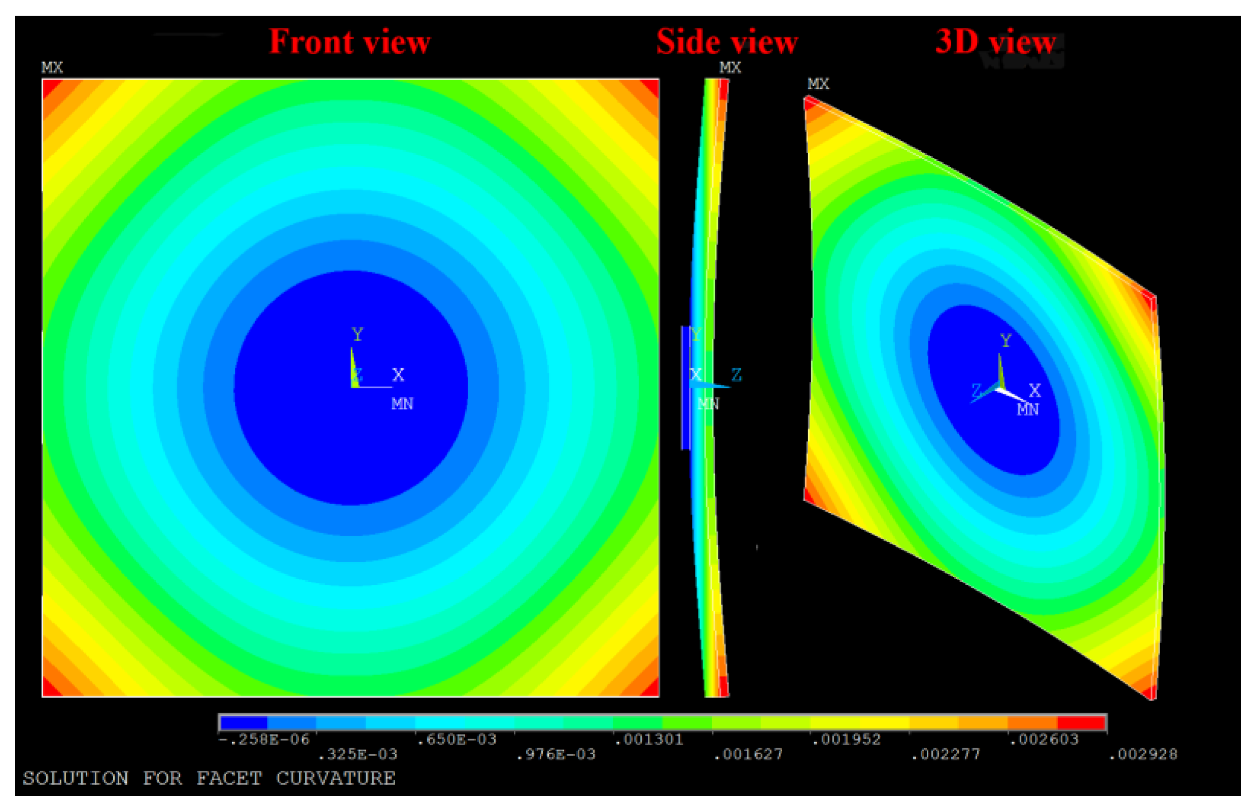
4.3. Slope Error of the Concentrator

The properties of concentrator facets are listed in

Table 3. Properties of the concentrator facet.

Name	Values
Diameter of connecting pad (mm)	600
Facet mirror thickness (mm)	4
Density (kg/m3)	2800
Young’s modulus (GPa)	75
Poisson ratio	0.25

. The concentrator facet is a square mirror with a side length of 300 mm. As illustrated in Figure 3a, the surface adjustment is achieved by pushing eight bolts numbered from 1 to 8, contacted in the rear of the mirror.

Table 4. Parameters of concentrator facets in simulation cases.

Name	Displacements of the Adjusting Bolts (mm)
	1	2	3	4	5	6	7	8
Facet a	2.58	1.29	2.58	1.29	2.58	1.29	2.58	1.29
Facet b	3.00	1.50	3.00	1.50	3.00	1.50	3.00	1.50
Facet c	2.60	1.20	2.60	1.20	2.60	1.20	2.60	1.20
Facet d	2.80	1.80	2.50	1.00	3.50	0.80	2.20	1.20
Facet e	An ideal revolution paraboloid with a focal distance of 3.8 m

provides five different facet shapes simulated in this section. The connecting pad fixed at the center of the facet are all with the diameter of 60 mm. It should be noted that if the facet is placed at the center of the concentrator, displacements of the adjusting bolts in facet a equal to sagitta lengths in an equivalent revolution paraboloid. Among those facets, facet a shows the closest curvature as the paraboloidal with the same focal. The displacements in facet e is measured data in practical.

Figure 8 gives the curved surface of facet a obtained by the FEM. From the result, the plane area is occurred at the center due to the displacement constraint of the connecting pieces. Along the direction from the center to the periphery, the circumferential curvature near the center changes similarly, and the gradient in curvature becomes larger near the outer circle. In the solar furnace, five forms of the facets’ ability to concentrate solar power show obvious differences in Figure 9. Facet e results in a cylindrical irradiance distribution. Its peak heat flux is 30.41 kW/m² and the spot is around 10 mm radius (where 90% of the solar power are collected). Concentrated heat flux results for facet a and facet c present the Gaussian distribution, normally seen in the practical cases. Their peak heat fluxes are 22.84 kW/m² and 19.91 kW/m², respectively. Under the same thermal power, those values decrease by 24.9% and 34.5% compared with that of facet e. When compared mutually, facet a’s ability to concentrate solar power is better than that of facet c, in terms of smaller spot size and higher peak heat flux. With the surface adjustment approach mentioned above, the curved surface of facet a is the most ideal one can be achieved in practical. From the rest simulation cases, adjusting bolts near four vertices of facet b push the mirror so hard that its surface is excessively deformed, and in result, the concentrated heat flux shows a multi-peak central symmetrical distribution with a minimum value at the center. As to facet d, its peak heat flux position slightly shifts from the center of the receiver surface with the value of 12.95 kW/m². The distribution is scattering and irregular in shape. In general, the displacements of adjusting bolts need to be controlled within the accuracy of millimeters, otherwise, the slope error resulted from the surface deformation would obviously reduce the facet’s concentrating ability.

4.4. Layout Error of the Concentrator

We have selected five kinds of concentrator layouts to analyze the influence of the layout error. The mirror arrays attached to four of them are, respectively, facet a, b, c, and e in Table 3. The last one is a continuous revolution paraboloid concentrator, taken as a reference in the theoretically ideal condition. The simulation results are presented in Figure 10.

The thermal power of the five cases on the receiver surface is equal. The green line synthetizes the reference case. As is intuitively expected, it has the minimum spot size with the diameter 50 mm, and the maximum peak heat flux is up to 6071 kW/m². The concentrator filled with facet e shows the second-best performance. Compared to the reference, its peak heat flux is decreased by 16.2%, and the concentrated irradiance is no longer a cylindrical distribution but occurs as the gradient decreases from the center to the periphery. However, those two cases might not be achievable in the practical situation. The most approaching result is a Gaussian heat flux distribution, as illustrated with the blue and yellow lines. Combined with conclusions in the previous section, even the focusing effect of single-piece facet in Table 3 has the obvious difference that the overall performance of the concentrator does not reflect the sum of their slope errors. That is to say, due to the layout error, the error influence caused by concentrator facets deformation is diminished at some point. The peak heat flux of layouts covered with facet a and facet c are reduced by 39.3% and 40.3%, respectively, which is still tantamount to more than 3000 suns of solar energy. It indicates a good optical performance for the solar furnace. Nonetheless, for the concentrator layout using facet e, the flux distribution keeps in a multi-peak shape and also the overall value is low, which further emphasizes the importance to ensure the accuracy of the displacements of adjusting bolts within 1~2 mm.

4.5. Tilt Error of Concentrator

As differing from the tilt error in the heliostat, for the concentrator, it is described in two orthogonal directions. The vertical title error range along $y_{c_j}$-axis is defined as $e_{cx}=2\cdot {\phi }_{c\max }$, and the horizontal along $x_{c_j}$-axis is defined as $e_{cy}=2\cdot {\psi }_{c\max }$. The radial angle ${\phi }_{c_j}$ and circumferential angle ${\psi }_{c_j}$ of the j-th concentrator facet’s tilt error are given by Equation (21), which is also a uniform randomness model. Here, ${\epsilon }_5$, ${\epsilon }_6$ ${\epsilon }_7$ ${\epsilon }_8$ are random numbers between 0 and 1.

$$\begin{array}{l}{\phi }_{c_j}=\mathrm{sign}\left({\epsilon }_5-0.5\right)\cdot \mathrm{atan}\left(\sqrt{{\epsilon }_6}\tan {\phi }_{c\max }\right)\\ {\psi }_{c_j}=\mathrm{sign}\left({\epsilon }_7-0.5\right)\cdot \mathrm{atan}\left(\sqrt{{\epsilon }_8}\tan {\psi }_{c\max }\right)\end{array}$$

(21)

It is observed from Figure 11 that as $e_{cx}$ increases, the concentrated heat flux gradually diverges along the $y_R$-axis, and the position of the peak heat flux slightly shifts vertically, and distribution along the $x_R$-axis maintains a good Gaussian shape, but values decreases. Likewise, the factor $e_{cy}$ has the same effect but in opposite direction. When tilt errors are less than 2 mrad, the performance of solar furnace is closed to that in the ideal; as tilt errors are less than 4 mrad, the concentrated heat flux distribution can still maintain a good Gaussian shape.

4.6. Comprehensive Factor Influence

Take an experimentally measured concentrated heat flux to analyze the comprehensive influence of four optical factors. The selected data was measured at 13:38 on 18th June 2015. At this moment, the measured DNI is 851 W/m², with the measured reflectance as ${\eta }_3=0.80$, ${\eta }_4=0.83$. From the simulation, it shows that gap loss in the heliostat is 5.3%, the sum of incoming rays’ overflowing and the gap loss in concentrator is 24.1%. The total number of traced rays is 1 × 10⁸, and 7.19 × 10⁷ of them reach the receiver surface. The cosine efficiency is ${\eta }_2=0.63$, and the shadow is ${\eta }_3=0.90$. From the discussions above, if factors in the optical system effect individually, it could attain the comparatively ideal working performance of the solar furnace when $e_h\le 4\mathrm{mrad}$ or using facet a or $e_{cx}\le 2\mathrm{mrad}$, $e_{cy}\le 2\mathrm{mrad}$, which coincides with the conclusion in reference [9] that the upper boundary of 4 mrad for optical errors can achieve the desirable structure design. Three forms of solar furnace used to study the comprehensive influence of errors are listed in

Table 5. Parameters of solar furnace with different errors.

Name	Tilt Error in Heliostat	Tilt Error in Concentrator	Concentrator Facet
Solar furnace a	$e_h=0\mathrm{mrad}$	$e_{cx}=0\mathrm{mrad}$, $e_{cy}=0\mathrm{mrad}$	Facet a
Solar furnace b	$e_h=4\mathrm{mrad}$	$e_{cx}=0\mathrm{mrad}$, $e_{cy}=2\mathrm{mrad}$	Facet a
Solar furnace c	$e_h=12\mathrm{mrad}$	$e_{cx}=3\mathrm{mrad}$, $e_{cy}=8\mathrm{mrad}$	Facet a

. Comparisons between the simulations and the experiment is given in Figure 12.

Solar furnace a represents the ideally optimal optical performance in the engineering practice for the present structure design. From the results, peak heat flux of solar furnace a, b, and c are 4036 kW/m², 2586 kW/m², and 1290 kW/m², respectively. The solar furnace b’s is 11.2% lower than that value of solar furnace a. It indicates that even each error can be well controlled, for the reason of the optical system demanding extremely high precision, the comprehensive influence of factors can obviously decrease the facility’s performance. For the solar furnace c in Figure 12a, the integral of the heat flux equals to the thermal power of 8.28 kW, which agrees with the value calculated by Equation (22). It can further verify the accuracy of the model.

$$P=\mathrm{DNI}\cdot S_H\cdot \frac{{\displaystyle \sum N_k}}{N_t}\cdot {\eta }_2\cdot {\eta }_3\cdot {\eta }_4\cdot {\eta }_5=8.29\mathrm{kW}$$

(22)

As shown in Figure 12a, the flux distribution in the simulation shows Gaussian shape, as the measured result presents. Their trend of gradient change and the shape and size of the spot are approximately similar. However, the overall heat flux values in the simulation are much higher than the experiment. In particular, the measured peak flux is 484 kW/m² and the thermal power is around 2.5 kW, which is 30% of that in the simulation. Apparently, there are lots of uncertainties unexpectedly involved in the practical system, more than the four factors focused on in the present work. Based on the comparisons in Figure 12b, there are several possible explanations given, as follows:

• In terms of simulation, the MCRT model mainly consider optical factors caused by facets, not including the heliostat tracking error, the pillar tilting, environmental factors, etc. The actual situation is impossible to be exactly duplicated. Therefore, there must be differences between the simulation and the experiment.
• The experimental measurement procedure is as follows: A CCD camera captures the spot on the Lambertian intercepted surface and outputs the greyscale image. The heat flux result is then exported by comparing to the dependence of brightness and grey value on the standard point where a microsensor real-time measuring. The accuracy of the measurement strongly depends on the microsensor’s calibration. Thus, the accuracy of the experimental results may also be open to question.
• The difference in results between the experiment and the simulation, in the other aspect, also indicates that the comprehensive influence from various factors has an obvious impact on the overall operating performance of solar furnace. The key to a higher optical behavior is controlling each error well within the allowable range.

5. Conclusions

This paper introduces both the optical structure design and the MCRT model for the solar furnace in detail. The optical structure design adopts one two-axis tracking heliostat and one faceted concentrator using the identical facets. In the concentrator, all curved facets are deformed to an approximate revolution paraboloid by adjusting bolts in the rear, and then attached to the frame orienting normal to their respective position. The result using the MCRT model agrees well with the available references, which could validate its accuracy. By analyzing the simulations, influences of four optical factors on the optical performance are discussed:

• The tilt error of heliostat affects the non-parallelism degree of the reflected sunlight. As the error increases, both the concentrated heat flux distribution and spot are diverging.
• The FEM is used to obtain the curved surface of concentrator facet. The slope error of the concentrator causes the mirror unit to become no longer an ideal surface, but rather complex and irregular under constraints. The error in the 1~2 mm could greatly reduce the concentration ability.
• The layout error occurs when facets attached to the concentrator frame share a similar curvature. Its existence will not enlarge the influence of the slope error.
• The tilt error of concentrator facets directly impacts on the focusing effect. As the tilt error increases in a certain direction, heat flux along the direction is scattering, while the orthogonal direction keeps in the Gaussian shape, but overall value decreases.

Based on the facility in Yanqing, Beijing, allowable ranges for corresponding errors effect individually are given: The tilt error of heliostat $e_h\le 4\mathrm{mrad}$; concentrator facets adopts facet a, in which displacements of adjusting bolts equal to sagitta lengths in the equivalent paraboloid; tilt error of concentrator $e_{cx}\le 2\mathrm{mrad}$ and $e_{cy}\le 2\mathrm{mrad}$. Besides, the comprehensive influence of the four factors has been studied. The study shows that even when controlling well for each optical factor within the allowable range, the optical performance of the solar furnace will drop significantly because of their coexistence. Compared with the experimentally measured concentrated heat flux, it indicates that there are still considerable uncertainties remained to be discussed in the further study. Besides, it is also worth to figure out how the optical factors influence the thermal behavior on the testing materials. Results in the present work are useful for the developers to have a better understanding of the influences of factors on the final result. It is helpful in the process of manufacture and assembling to attain the optimal performance of the solar furnace.

References

1. Trefilov, V.; Schur, D.; Pishuk, V.; Zaginaichenko, S.; Choba, A.; Nagornaya, N. The solar furnaces for scientific and technological investigation. Renew. Energy 1999, 16, 757–760. [Google Scholar] [CrossRef]
2. Oliveira, F.A.C.; Fernandes, J.C.; Badie, J.-M.; Granier, B.; Rosa, L.G.; Shohoji, N. High meta-stability of tungsten sub-carbide W2C formed from tungsten/carbon powder mixture during eruptive heating in a solar furnace. Int. J. Refract. Met. Hard Mater. 2007, 25, 101–106. [Google Scholar] [CrossRef]
3. Villafán-Vidales, H.; Arancibia-Bulnes, C.; Riveros-Rosas, D.; Romero-Paredes, H.; Estrada, C. An overview of the solar thermochemical processes for hydrogen and syngas production: Reactors, and facilities. Renew. Sustain. Energy Rev. 2017, 75, 894–908. [Google Scholar] [CrossRef]
4. Guillot, E.; Rodriguez, R.; Boullet, N.; Sans, J.-L. Some details about the third rejuvenation of the 1000 kWth solar furnace in Odeillo: Extreme performance heliostats. AIP Conf. Proc. 2018, 2033, 040016. [Google Scholar]
5. Abdurakhmanov, A.A.; Zainutdinova, K.K.; Mamatkosimov, M.A.; Paizullakhanov, M.S.; Saragoza, G. Solar technologies in Uzbekistan: State, priorities, and perspectives of development. Appl. Sol. Energy 2012, 48, 84–91. [Google Scholar] [CrossRef]
6. Rodriguez, J.; Cañadas, I.; Zarza, E. New PSA high concentration solar furnace SF40. AIP Conf. Proc. 2016, 1734, 070028. [Google Scholar] [Green Version]
7. Lee, H.; Chai, K.; Kim, J.; Lee, S.; Yoon, H.; Yu, C.; Kang, Y. Optical performance evaluation of a solar furnace by measuring the highly concentrated solar flux. Energy 2014, 66, 63–69. [Google Scholar] [CrossRef]
8. Zhang, X.; Cui, Z.; Zhang, J.; Bai, F.; Wang, Z. Optical performance analysis of an innovative linear focus secondary trough solar concentrating system. Front. Energy 2018, 13, 590–596. [Google Scholar] [CrossRef]
9. Riveros-Rosas, D.; Herrera-Vázquez, J.; Pérez-Rábago, C.; Bulnes, C.A.A.; Vázquez-Montiel, S.; Sanchez-Gonzalez, M.; Granados-Agustín, F.; Jaramillo, O.; Estrada, C.; Jaramillo, O. Optical design of a high radiative flux solar furnace for Mexico. Sol. Energy 2010, 84, 792–800. [Google Scholar] [CrossRef]
10. Neumann, A.; Groer, U. Experimenting with concentrated sunlight using the DLR solar furnace. Sol. Energy 1996, 58, 181–190. [Google Scholar] [CrossRef]
11. Jafrancesco, D.; Sansoni, P.; Francini, F.; Contento, G.; Cancro, C.; Privato, C.; Graditi, G.; Ferruzzi, D.; Mercatelli, L.; Sani, E.; et al. Mirrors array for a solar furnace: Optical analysis and simulation results. Renew. Energy 2014, 63, 263–271. [Google Scholar] [CrossRef]
12. Ballestrín, J.; Monterreal, R. Hybrid heat flux measurement system for solar central receiver evaluation. Energy 2004, 29, 915–924. [Google Scholar] [CrossRef]
13. Li, Z.; Tang, D.; Du, J.; Li, T. Study on the radiation flux and temperature distributions of the concentrator—Receiver system in a solar dish/Stirling power facility. Appl. Therm. Eng. 2011, 31, 1780–1789. [Google Scholar] [CrossRef]
14. Zhao, D.; Xu, E.; Wang, Z.; Yu, Q.; Xu, L.; Zhu, L. Influences of installation and tracking errors on the optical performance of a solar parabolic trough collector. Renew. Energy 2016, 94, 197–212. [Google Scholar] [CrossRef]
15. Shuai, Y.; Xia, X.-L.; Tan, H.-P. Radiation performance of dish solar concentrator/cavity receiver systems. Sol. Energy 2008, 82, 13–21. [Google Scholar] [CrossRef]
16. Zou, B.; Dong, J.; Yao, Y.; Jiang, Y. A detailed study on the optical performance of parabolic trough solar collectors with Monte Carlo Ray Tracing method based on theoretical analysis. Sol. Energy 2017, 147, 189–201. [Google Scholar] [CrossRef]
17. Bonanos, A.M. Error analysis for concentrated solar collectors. J. Renew. Sustain. Energy 2012, 4, 063125. [Google Scholar] [CrossRef]
18. Meyen, S.; Lupfert, E.; DLR Gernam Aerospace Center; Ciemat, A.F.-G.; Nrel, C.K. Standardization of Solar Mirror Reflectance Measurements—Round Robin Test; National Renewable Energy Lab. (NREL): Golden, CO, USA, 2010.
19. Meyen, S.; Lüpfert, E.; Pernpeintner, J.; Fend, T.; Schiricke, B. Optical Characterization of Reflector Material for Concentrating Solar Power Technology. In SolarPaces Conference. 2009. Available online: https://www.google.com/url?sa=t&rct=j&q=&esrc=s&source=web&cd=1&ved=2ahUKEwir9tCr55_lAhVnzIsBHV8eD48QFjAAegQIAhAC&url=http%3A%2F%2Felib.dlr.de%2F61684%2F1%2FSolarPaces2009_Mirror-Characterisation.pdf&usg=AOvVaw29cvWfKwbxWpYCBZeAaa_f (accessed on 15 October 2019).
20. Guo, M.; Wang, Z.; Zhang, J.; Sun, F.; Zhang, X. Accurate altitude—Azimuth tracking angle formulas for a heliostat with mirror—Pivot offset and other fixed geometrical errors. Sol. Energy 2011, 85, 1091–1100. [Google Scholar] [CrossRef]
21. Wang, F.; Bai, F.; Wang, T.; Li, Q.; Wang, Z. Experimental study of a single quartz tube solid particle air receiver. Sol. Energy 2016, 123, 185–205. [Google Scholar] [CrossRef]
22. Ma, L.; Wang, Z.; Lei, D.; Xu, L. Establishment, Validation, and Application of a Comprehensive Thermal Hydraulic Model for a Parabolic Trough Solar Field. Energies 2019, 12, 3161. [Google Scholar] [CrossRef]
23. Duffie, J.A.; Beckman, W.A. Solar Engineering of Thermal Processes; Wiley: Hoboken, NJ, USA, 2013; p. 23. [Google Scholar]
24. Xu, Y.; Cui, K.; Liu, D. The development of a software for solar radiation and its verification by the measurement results on the spot. Energy Technol. 2002, 23, 237–239. [Google Scholar]
25. Evans, D. On the performance of cylindrical parabolic solar concentrators with flat absorbers. Sol. Energy 1977, 19, 379–385. [Google Scholar] [CrossRef]
Figure 1. Schematic diagram of the solar furnace and coordinate systems.
Energies 12 03933 g001
Figure 2. Schematic diagram of a heliostat facet.
Energies 12 03933 g002
Figure 3. Backside of a concentrator facet structure: (a) Schematic diagram of a facet; (b) Picture of a facet.
Energies 12 03933 g003
Figure 4. Schematic of a concentrator facet.
Energies 12 03933 g004
Figure 5. Validation of the Monte Carlo ray tracing MCRT model: (a) Simulated concentrated heat flux; (b) Comparisons between the present work and the reference.
Energies 12 03933 g005
Figure 6. Solar furnace in Yanqing, Beijing: (a) Heliostat; (b) Concentrator and receiver.
Energies 12 03933 g006
Figure 7. Influence of the tilt error of the heliostat.
Energies 12 03933 g007
Figure 8. z-axis displacements color mapping of facet a.
Energies 12 03933 g008
Figure 9. Comparisons of concentrator facets on the concentrating ability.
Energies 12 03933 g009
Figure 10. Comparisons of center heat flux distribution of different concentrator layouts.
Energies 12 03933 g010
Figure 11. Influences of the tilt error of concentrator: (a) Along the vertical direction; (b) Along the horizontal direction.
Energies 12 03933 g011
Figure 12. Evaluation of the solar furnace in Yanqing, Beijing: (a) Comparison of concentrated heat flux distribution between the experiment and solar furnace c; (b) Comparisons of the center heat flux distribution.
Energies 12 03933 g012