Calculation of Ion Flow Field of Monopolar Transmission Line in Corona Cage Including the Effect of Wind

Abstract

In this work, the ion flow field of a monopolar transmission line inside the corona cage of a square cross-section is iteratively calculated concerning the effects of wind. The electric field distribution is solved analytically using the charge simulation method (CSM). Meanwhile, the upwind finite volume method (UFVM) with 2nd order accuracy is presented for the distribution of space charge density. Additionally, a dual mesh grid is established in the calculation domain, the interlaced geometric construction of the mesh assures a quick and effective convergence rate. In the final part, a reduced-scaled experiment is designed to examine the feasibility and accuracy of this approach, electric field and ion current density on the bottom side are measured by field mills and Wilson plates. The data numerically computed fits well with that acquired by measurement.

1. Introduction

In operating HVDC transmission lines of a power system, the phenomenon of corona discharge is a leading cause of radiation interference (RI), noise interference (NI), and corona loss (CL) [1]. Thus, investigation on the ion flow field distributed around the conductors receives considerable attention in the design of HVDC transmission lines.

Commonly, one of the main obstacles in solving the ion flow field is the nonlinearity between the electric field and space charge density. The vast majority of solutions calculate the electric field and the space charge density iteratively and the iteration process ends once the criteria are met. In the meantime, wind flow affects the distribution of the electric field around transmission lines to certain degree as well. All the above-mentioned issues increase the difficulty of calculating the ion flow field.

In the past few decades, research on the ion flow field calculation has varied in terms of the methods utilized to calculate the electric field and the space charge density in the domain of interest.

With regard to the electric field, Janischewskyj and Gela [2] introduced finite element method (FEM) to solve the electric field numerically; afterwards, this method was frequently adopted and well-developed. In 1983, Takuma et al. [3] applied CSM to calculate the nominal electric field without space charge, while FEM was used to solve the electric field induced by space charges. Since then, this approach has been broadly applied in electric field calculation [4,5]. CSM offers satisfactory accuracy, whereas the calculation domain is restricted to an infinite field above the ground or axisymmetric structure. Simultaneously, a drawback of FEM is that the accuracy of the electric field close to the conductor surface is not as expected because of the steep gradient.

In regard to the calculation of space charge density, method of characteristics (MOC) is diffusely utilized [6,7,8,9,10], space charge density is calculated along electric field lines with given initial charge density on the conductor surface. This approach relies on the Deustch’s assumption, which assumes the space charge affects the amplitude of an electric field rather than its direction. Xiao calculated the ion flow field around a cross-over transmission line in the 3D domain with the MOC method. However, the effectiveness of this method is unsatisfactory if the influence of wind flow is under consideration. Lu et al. [11] proposed an upwind FEM, which avoids non-physical instability of the numerical calculation. Zhou et al. [12] induced upwind weighting function to FEM for the purpose of eliminating the oscillations in simulation of charge conservation. Levin [13] established dual mesh based on the triangulation grid in calculation domain; the new mesh is called donor cell and the space charge density is hereby solved in accordance with Gauss’ Law. Then, upwind the FVM method were used in several research projects [5,14,15,16,17] in which the numerical stability, effectiveness, and accuracy of the solution process was improved substantially. Yang et al. [18] proposed an upstream meshless method to solve the current continuity equation.

For the purpose of implementing an indoor experiment and control of environmental parameters, a corona cage is designed in where the phenomenon of corona discharge initializes on a relatively lower voltage level. Bian et al. [19] and Lekganyane et al. [20] investigated the ion flow field in a square cross-section cage and compared the result with that of an indoor test line; Zhou et al. [8] presented a comprehensive study on the ion flow field distribution in a cylindrical cage employing a mesh-based method and MOC. However, there is paucity of published research concerning the effect of wind flow on the corona discharge of corona cage.

However, solution of the ion flow field generally concerns the numerical stability, calculation accuracy and the impact of wind flow. The referenced articles barely meet these requirements at the same time. Therefore, it is necessary to develop a method that offers a quick, stable, and accurate solution of ion flow field.

In this paper, the calculation domain is tessellated in the form of a dual mesh. Next, CSM is utilized for a nominal electric field in the absence of space charges. Simultaneously, electric fields generated by space charges is available if the space charges density is known, by this means, the accuracy of the calculated field is guaranteed even on the conductor surface. The 2nd order upwind FVM is employed to calculate the space charge density distribution. Eventually, the calculated result is validated with that derived by experiments.

The importance and originality of this study consists of the nominal electric field in a square cross-section being solved by means of proper placement of the simulation charges, the more accurate solution of space charge density distribution involving the impact from wind flow, as well as the applicability of this approach in presence of wind flow. The calculation process provides rapid convergence rate as the analytically calculated electric field is less time-consuming compared to the traditional method using FEM.

2. Mathematical Description

2.1. Governing Equations and Simplifying Assumption

Generally, the ion flow field in the ambient of conductor is governed by Poisson’s equation and the current density conservation equation [3]:

$$\{\begin{array}{l}\nabla \mathit{E}=-{\rho }^{-}/{\epsilon }_0\\ \nabla \cdot {\mathit{J}}^{-}=0\\ {\mathit{J}}^{-}={\rho }^{-}(b\mathit{E}+\mathit{W})\end{array}$$

(1)

where,

• b is the ion mobility, 1.5 × 10⁻⁴, m²/V/s;
• E is the electric field, V/m;
• ρ is the negative space charge density, C/m³;
• J⁻ is the negative ion current density vector, A/m²;
• W is the wind velocity vector, m/s; and
• ε₀ is the permittivity of air equals 8.854 × 10⁻¹², F/m.

Further, certain assumptions are proposed in advance in order to reduce the complexity of calculation and acquire satisfactory precision:

(a)

The thin ionization layer close to the conductor surface is neglected;

(b)

The ion mobility remains unchanged throughout the solution process;

(c)

Influence exerted by ion diffusion is ignored;

(d)

Kaptzov’s assumption [21] which presumes the electric field on conductor surface remains constant after the applied voltage reaches the onset value is adopted.

2.2. Boundary Conditions

Before proceeding to the solution process. Boundary conditions and initial conditions of the calculation domain are listed in

Table 1. Boundary conditions and initial conditions.

Distribution Variables	Conductor Surface	Cage Wall
Electric potential	Vapp	0
Space-charge density	ρs	$\frac{\partial \rho }{\partial n}$
Electric field	Eon	$\frac{\partial E}{\partial n}$

.

where,

• V_app is the voltage supplied on the conductor, V;
• ρ_s refers to the space charge density on the conductor surface, C/m³;
• E_on is the onset electric field, V/m; and
• E_on is assumed to be constant on the conductor surface according to Kaptzov’s assumption, the explicit value is attained using Peek’s empirical formula [22]:

  $$E_{\mathrm{on}}=30m(1+\sqrt{\frac{0.0906}{r}})$$

  (2)

where,

• m is the roughness factor set to 0.65; and
• r is the radius of the conductor, m.

An appropriate guess of the initial value of the charge density on conductor surface determines the accuracy of the result and diminishes the iteration process. The empirical formula introduced in [23] is referred to in this paper:

$${\rho }_s=\frac{E_g}{E_c}\frac{8{\epsilon }_0{V}_c(V_{\mathit{app}}-V_c)}{r{H}_{con}(5-4V_c/V_{app})}$$

(3)

where,

• E_g is the ground level electric field under the conductor, V/m;
• E_c is the nominal electric field on the conductor, V/m;
• V_c is the onset voltage of the conductor, V;
• V_con is the conductor voltage, V; and
• H_con is the height of the conductor, m.

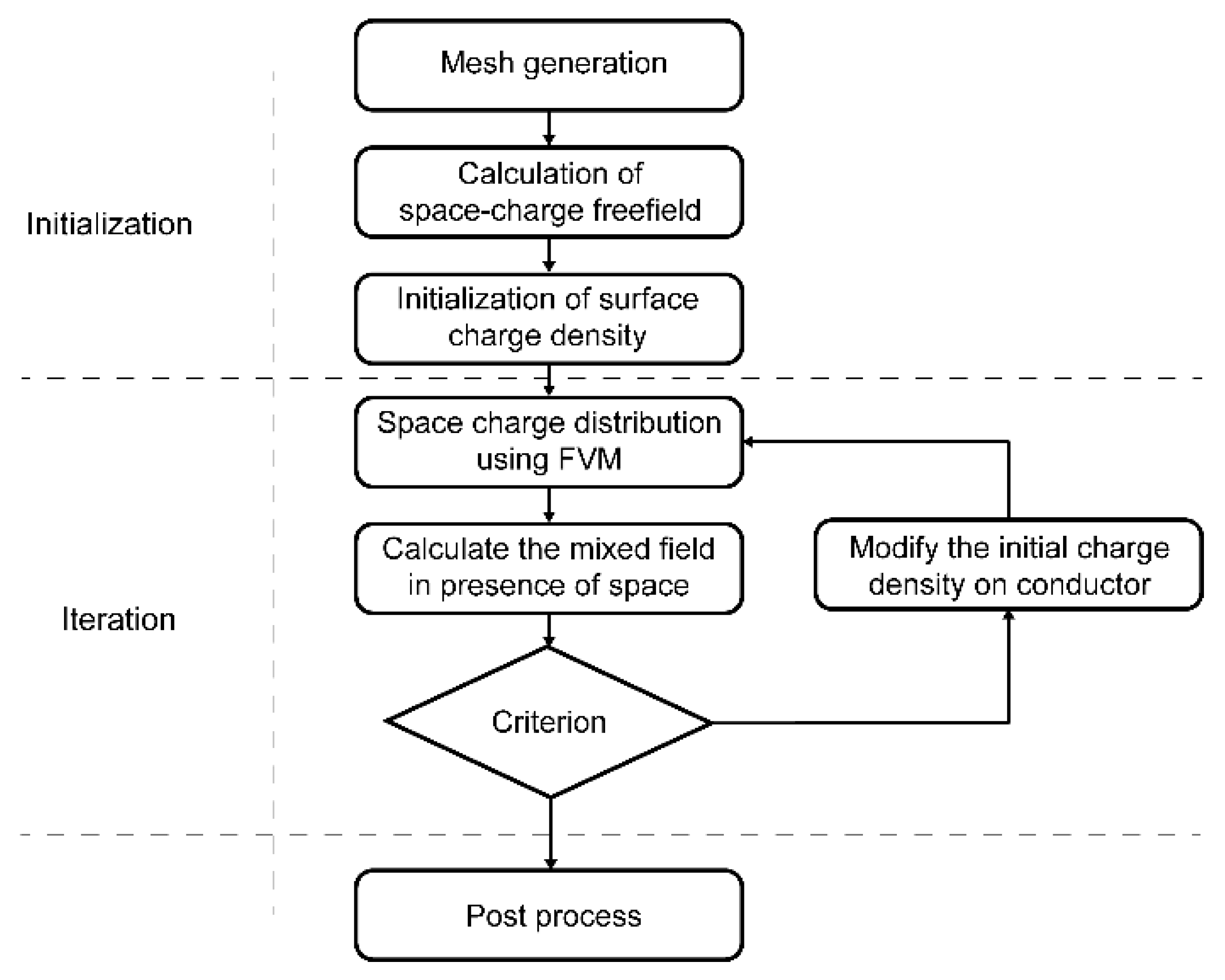
Takuma [3] assumes that the initial charge density is evenly distributed on the conductor surface, yet it is not suitable for the situation where the transmission line is placed inside corona with a square cross-section cage. Because distances between the conductor surface to the cage wall are diverse, which differs from the situation above the ground or in the coaxial cage. Hence, in this work, charge density is set to be linearly dependent on E_c. To be specific, for each node on the conductor surface, E_c is calculated by CSM, neglecting space charges. Thus, the initial charge density of this node is achieved by substitute corresponding E_c into Equation (3).

3. Solution Process

The distributions of electric field and space charge density are solved iteratively, in this process, the initial charge density on the conductor surface is updated in each iteration in case that the condition of convergence is not satisfied. The detailed procedure is organized and illustrated in Figure 1.

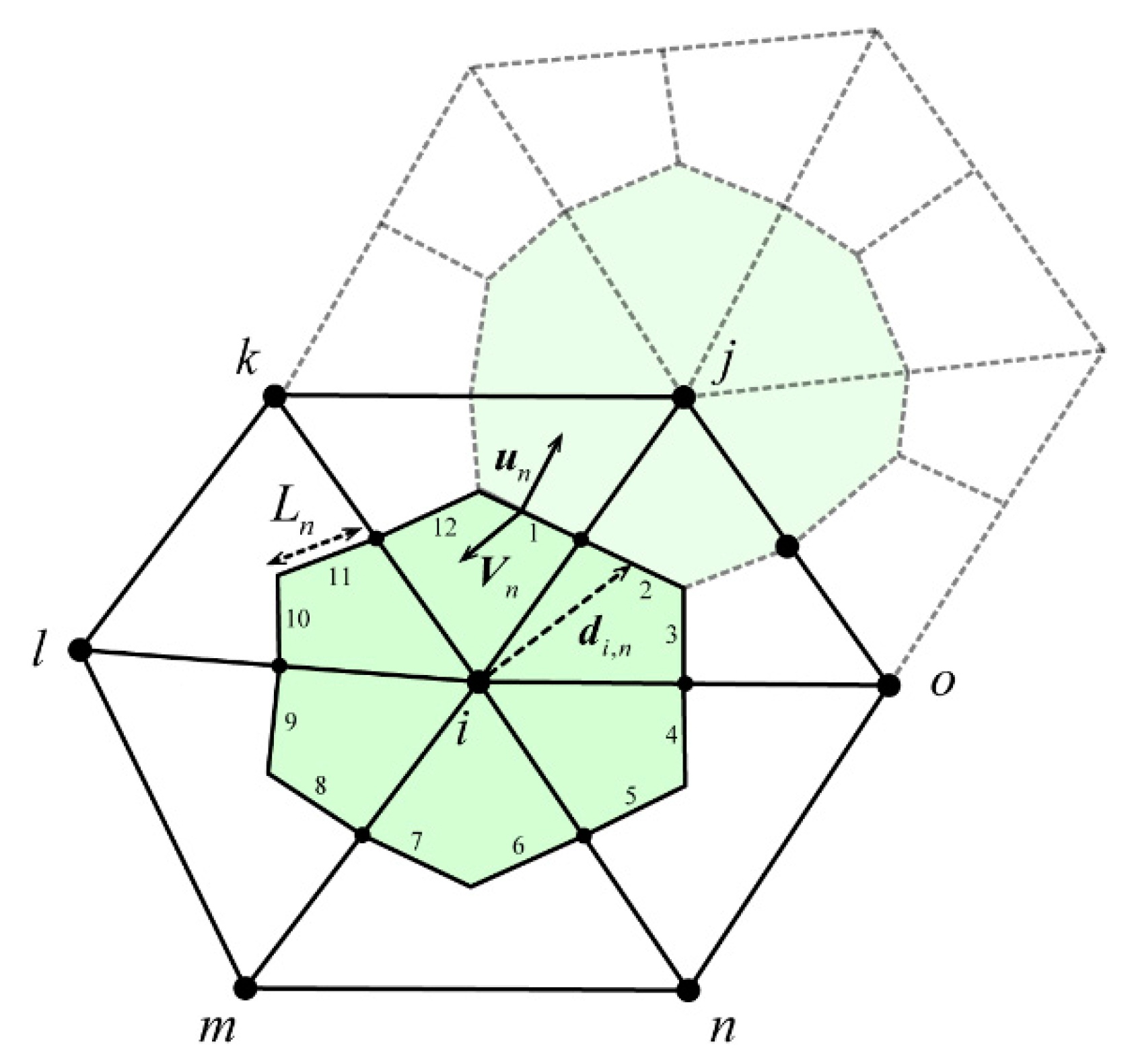
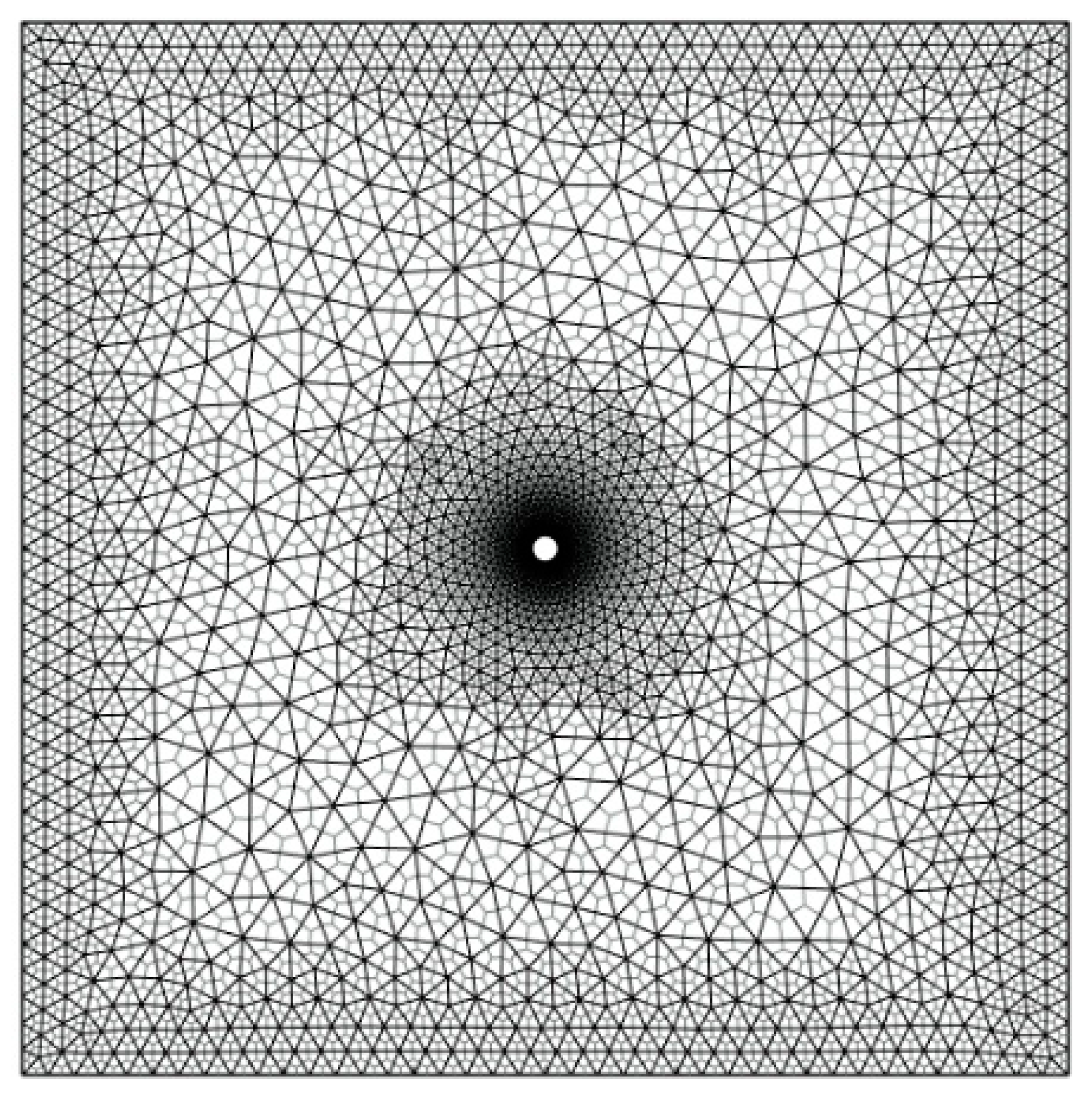
3.1. Discretization of Calculation Domain

The calculation is conducted in the 2D cross-section of the cage, and the calculation domain is divided in form of dual mesh. Specifically, a Delaunay Triangular mesh is generated in the first place; after that, polygon cells are constructed via connecting the barycenter and the midpoints of triangular cell edges, which share common vertexes [24].

The meshing of the calculation domain is demonstrated in Figure 2. Meshing of the area in the vicinity of the conductor surface and the cage wall are finer in the cause of the need of more accurate calculation results. As a result of the grid independency test, the difference of the calculated result is less than 1%, while the domain is tessellated into 1879 cells.

Since the electric field is calculated analytically, the electric field in each single point can be calculated defectively. Regarding to the space charge density, they are stored in the nodes of the triangulation. The effectiveness of the solution process is ensured resulting from the interlaced meshing scheme.

3.2. Calculation of Electric Field

The calculation of electric field composes of two parts: the nominal field and the field induced by space charges.

Regarding the nominal field to be calculated by CSM, there are 40 simulation charges equally distributed inside the conductor.

In contrast to the circumstance of outdoor lines above the ground, extra simulation charges are placed outside the cage wall to maintain the zero potential of the grounded cage wall; as a result, as demonstrated in Figure 3, there are 160 simulation charges equidistantly arranged with interval d_c, the perpendicular distance between the cage wall and simulation charges are two times of d_c. Image charges are placed symmetrically in the opposite sides of the ground. The match points are placed right on the conductors and corona walls, respectively.

According to the principle of CSM, values of the simulation charges must ensure the potential on the conductor surface and cage wall to be V_app and zero. Thus, coefficient equations are listed below:

$$\{\begin{array}{l}{P}_{cond}\cdot Q_{cond}+P_{cage}\cdot Q_{cage}=V_{app}\\ P_{cond}^{\prime }\cdot Q_{cond}+P_{cage}^{\prime }\cdot Q_{cage}=0\end{array}$$

(4)

where Q_cond and Q_cage are simulation charges of the conductor and cage, P_cond, P_cage are the potential coefficients regarding the conductor surface, and P′_cond, P′_cage are the potential coefficients for the cage wall.

The nominal electric field is therefore obtained by superposing the field caused by simulation charges. The space charges-induced field can be calculated if the space charges are known. Accordingly, the ion flow field is available as follows:

$$E_{\mathrm{m}}={\displaystyle \sum _i\frac{Q_i}{4\pi {\epsilon }_0}}\left(\frac{\stackrel{\rightharpoonup }{r_i}}{r_i^2}-\frac{\stackrel{\rightharpoonup }{r_i^{\prime }}}{r_i^{\prime 2}}\right)+{\displaystyle \sum _j{\displaystyle \underset{s_j}{\int }\frac{{\rho }_j}{4\pi {\epsilon }_0}}}\left(\frac{\stackrel{\rightharpoonup }{r_j}}{r_j^2}-\frac{\stackrel{\rightharpoonup }{r_j^{\prime }}}{r_j^{\prime 2}}\right)d{s}_j$$

(5)

where,

• s_j is the area of the polygon cell, m³;
• r_i and r_j are the distances between the observation point to the source, m;
• $r_i^{\prime }$ and $r_j^{\prime }$ are the distances between the observation point to the image points, m;
• Q_i are the simulation charges consist of Q_cond and Q_cage, C; and
• ρ_j is the charge density on triangulation nodes, C/m³.

3.3. Calculation of Ion Current Density

FVM ensures the maximum principle of charge density on cell boundaries resulting in numerical stability in the calculation process. Additionally, the upwind scheme satisfies the physical fact that the migration of space charges is affected by upwind stream only [25]. Particularly, this method is feasible for calculation in the presence of wind flow.

By substituting Equation (3) into Equation (2), following equation is obtained:

$$\nabla \cdot [{\rho }^{-}(b\mathit{E}+\mathit{W})]=0$$

(6)

Afterwards, Equation (6) is converted to integral form:

$${\displaystyle {\iint }_s\rho (b\mathit{E}+\mathit{W})dl=0}$$

(7)

where,

• s and l are the area and boundary of the cell.

Next, Equation (7) is rewritten in the form of linear equations in the light of Figure 4:

$${\displaystyle {\sum }_{n=1}^n\rho {\mathit{V}}_n{L}_n}=0$$

(8)

where,

• V_n = bE_n + W_n, E_n and W_n are the outward normal component of electric field and wind speed on cell edges, and
• L_n is the length of the ith cell; and
• n presents the serial number of the edges.

Finally, a system of linear equations is established and the distribution of charge density is therefore achieved.

Normally, charge density is defined as the average value of adjacent nodes [15], or determined by the upwind scheme. Nevertheless, these methods are only of 1st order accuracy which is insufficient for engineering requirements.

With an aim to promote the accuracy of space charge density, a 2nd order upwind scheme is utilized. Charge densities on the edges are solved directly. Apparently, the charge densities on cell edges can be expressed according to the Taylor series expansion as Figure 4:

$$\{\begin{array}{l}{\rho }_{i,n}={\rho }_i+\nabla {\rho }_{i,n}\cdot {\mathit{d}}_{i,n}if{\mathit{V}}_n\cdot {\mathit{u}}_n>0\\ {\rho }_{i,n}={\rho }_n+\nabla {\rho }_{n,i}\cdot {\mathit{d}}_{n,i}if{\mathit{V}}_n\cdot {\mathit{u}}_n<0\end{array}$$

(9)

where,

• ρ_i,n is the charge density on the edge, C/m³;
• d_i,n is the vector direct from the ith node to the corresponding neighboring nodes; and
• ∇ρ_i,n and ∇ρ_n,i are the gradient of corresponding upwind node.

For the known charge densities on the ith node and its adjacent nodes, the following over determined matrix equation can be established; thus, the gradient of charge density on the ith node is obtained:

$${\left|\begin{array}{cc}\Delta x_1& \Delta y_1\\ \Delta x_2& \Delta y_2\\ \dots & \dots \\ \Delta x_n& \Delta y_n\end{array}\right|}_{A_n{}_{\times 2}}\times {\left|\begin{array}{l}\frac{\partial {\rho }_i}{\partial x}\\ \frac{\partial {\rho }_i}{\partial y}\end{array}\right|}_{X_{2\times 1}}={\left|\begin{array}{c}{\rho }_i-{\rho }_1\\ {\rho }_i-{\rho }_2\\ \dots \\ {\rho }_i-{\rho }_n\end{array}\right|}_{B_{n\times 1}}$$

(10)

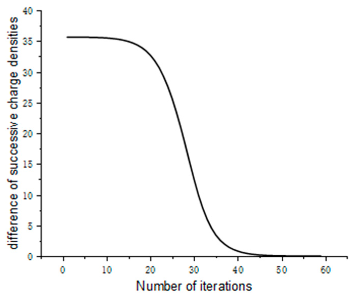
3.4. Terminal Criteria and Initial Charge Density

The iteration procedure will terminate while the following conditions are met.

$$\frac{E_c-E_0}{E_0}<{\delta }_E$$

(11)

$$\frac{1}{N}{\displaystyle \sum _{i=1}^N\frac{\left|{\rho }_{m,i}-{\rho }_{m-1,i}\right|}{\left|{\rho }_{m-1,i}\right|}}<{\delta }_{\rho }$$

(12)

where,

• δ_E and δ_ρ are relative terminal criteria;
• E_c is the electric field on conductor surface, V/m; and
• ρ_m,i and ρ_m−1,i are consecutive space charge densities of the iteration process in ith cell, C/m³.

However, the initial charge densities on the conductor surface need to be modified in each iteration so as to maintain the electric field on conductor surface as E₀, the principle abides by the following equation:

$${\rho }_{m-1}={\rho }_m\left(1+\mu \cdot \frac{E_c-E_0}{E_c+E_0}\right)$$

(13)

where,

• ρ_m−1, ρ_m are charge densities of two consecutive iteration on conductor surface, C/m³; and
• μ is the acceleration factor equals to two.

Distributions of the space charge density of different wind speed are indicated in Figure 5. The convergence rate of the calculation under −120 kV voltage supply and 10 m/s wind speed is shown in Figure 6; the iteration process has a good convergence and ends after about 45 times of iteration. It takes fewer than 10 min since the coefficient matrix of the electric field is prepared once and for all.

4. Validation

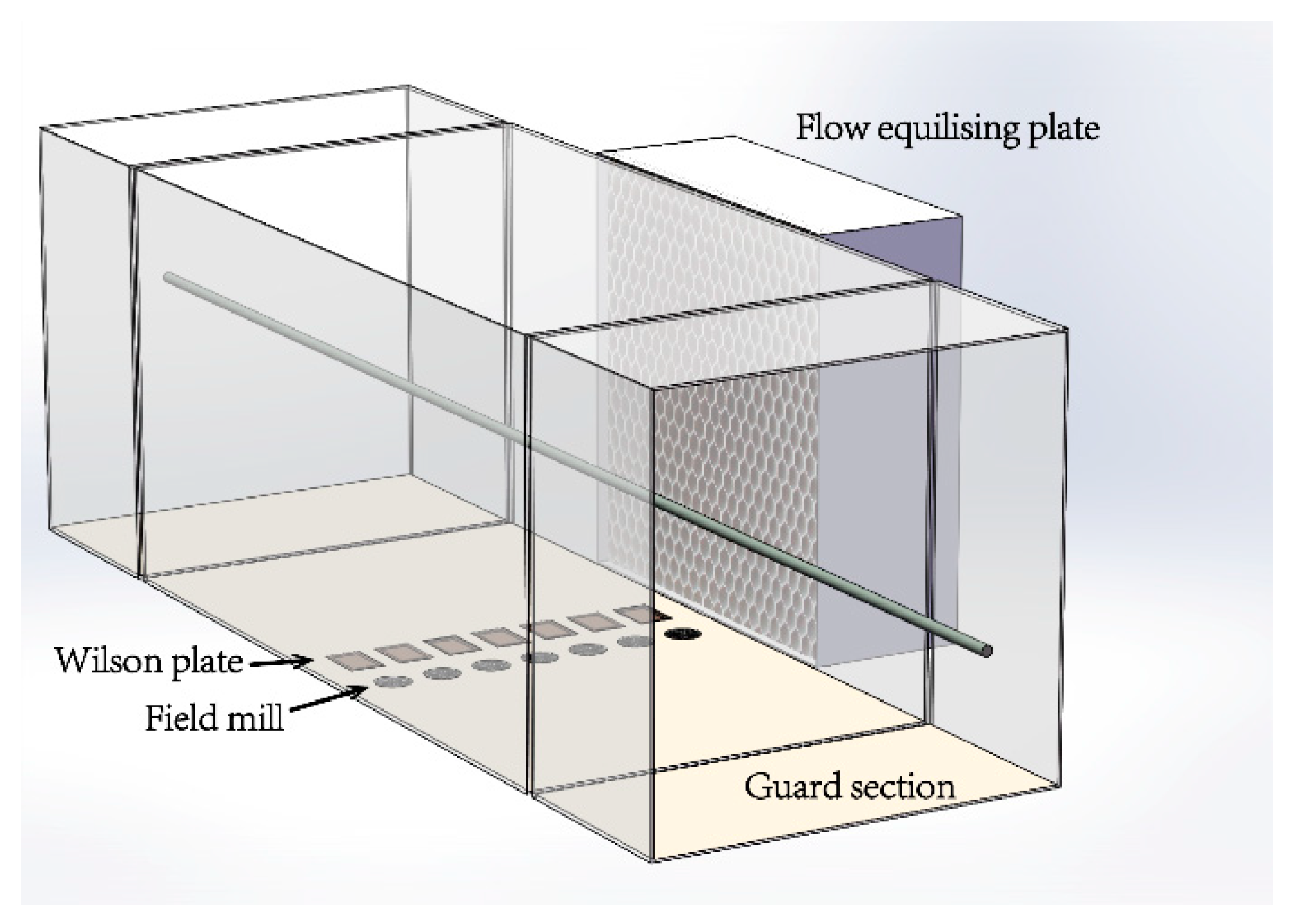
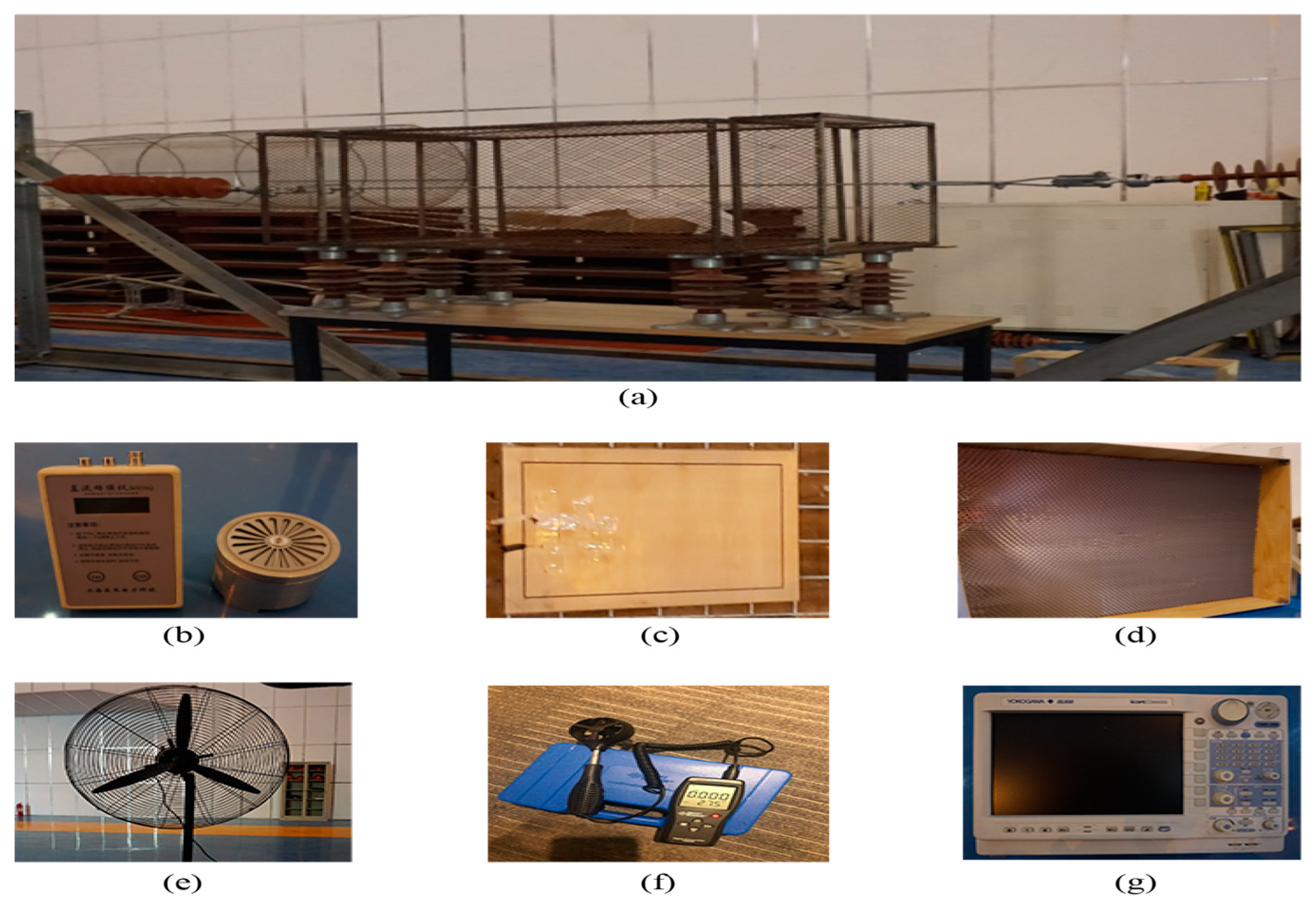
4.1. Design of the Experiment

The corona cage is frequently used, which offers much more intensive field strength on relatively low voltage level. The reduced size of experimental facility enables indoor experiments.

The dimension of the main section of the corona cage is 1500 × 800 × 800 (mm), there are two guard sections size at 300 × 800 × 800 (mm) in order to eliminate the impact results from end effect [26]. The conductor of 10 mm radius is hung along the center of the cross-section, and the two ends of the conductor are fixed on a steel frame with two composite insulators as a connection. The schematic diagram and experimental equipment are indicated in Figure 7 and Figure 8.

Seven Wilson plates and field mills are parallelly laid on the bottom side of the cage equidistantly for the measurement of ion current density and electric field.

Yokogawa scope coder DL 850 is used to record sampling signals of the ion flow current collected by Wilson plates, this equipment provides high sampling rate which is up to 100 Ms/s and enables continuous synchronous measurement of multi-channel.

The voltage was supported by a DC source with fluctuation less than 5%. The experiment was conducted at standard air pressure in a high voltage laboratory. The relative humidity was 20% to 30% and the temperature ranged from 10 °C to 15 °C.

An adjustable speed fan with four gears is placed next to the cage, facing one side of the cage, and it provides lateral wind speed of 0–10 m/s. The impact of flow divergence is moderated by a flow equalizing plate, the wind speed is measured by a digital high precision anemometer (AS-8336). The desired wind speed is achieved by adjusting the gear and distance between the fan and the equalizing plate. Since even distribution of the wind speed is the prerequisite of the experiment, wind speed values of 16 points are measured in the cross-section of the cage. The measurement shows that the standard deviation of wind speeds is less than 5%. The average measured result is demonstrated in Figure 9.

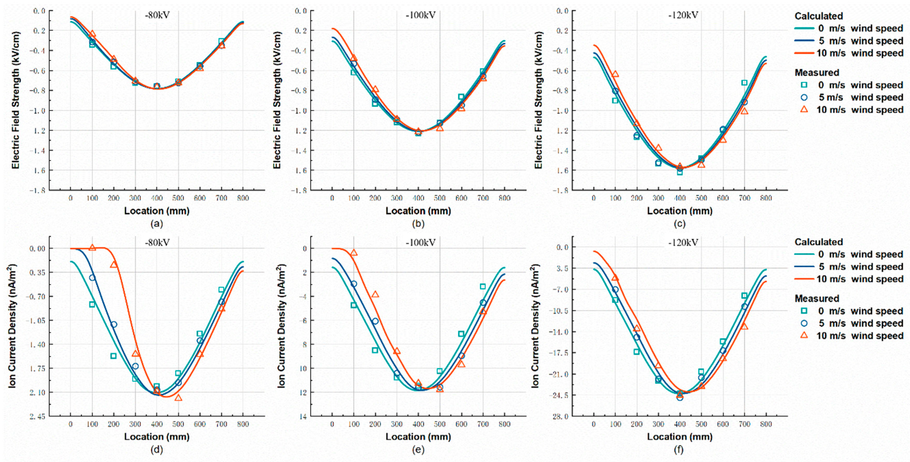
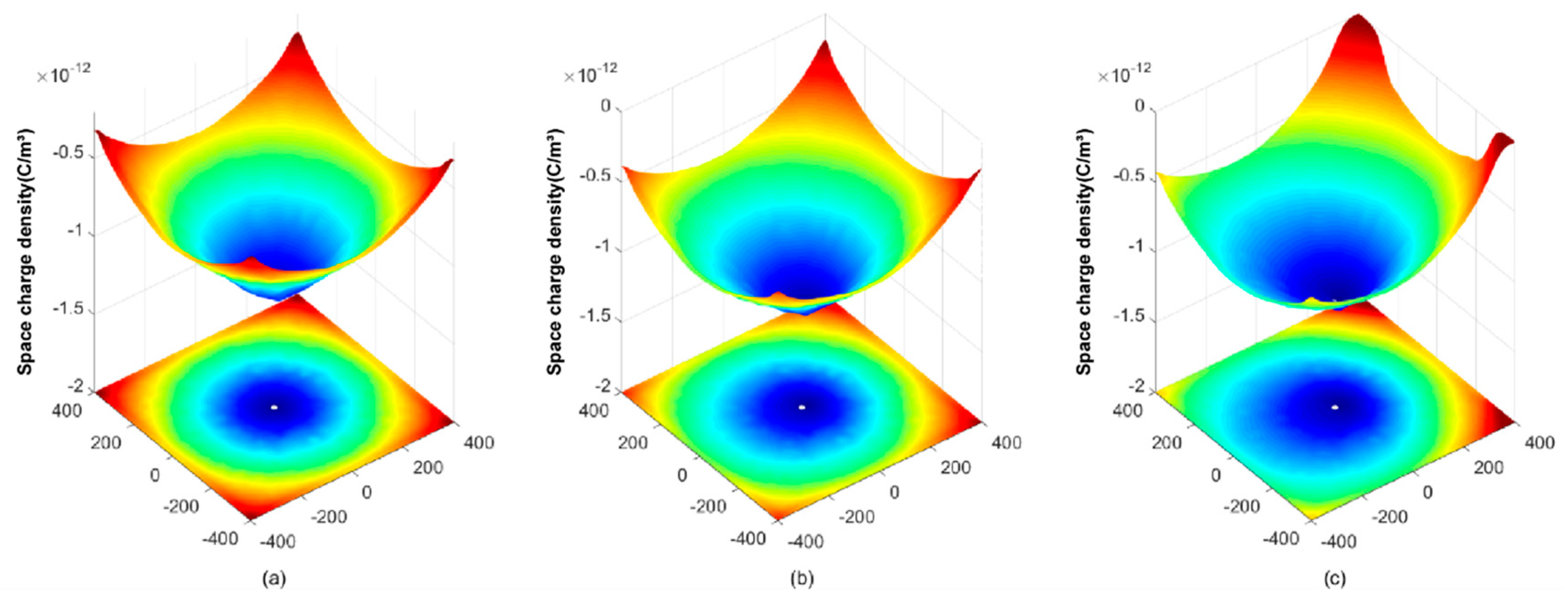
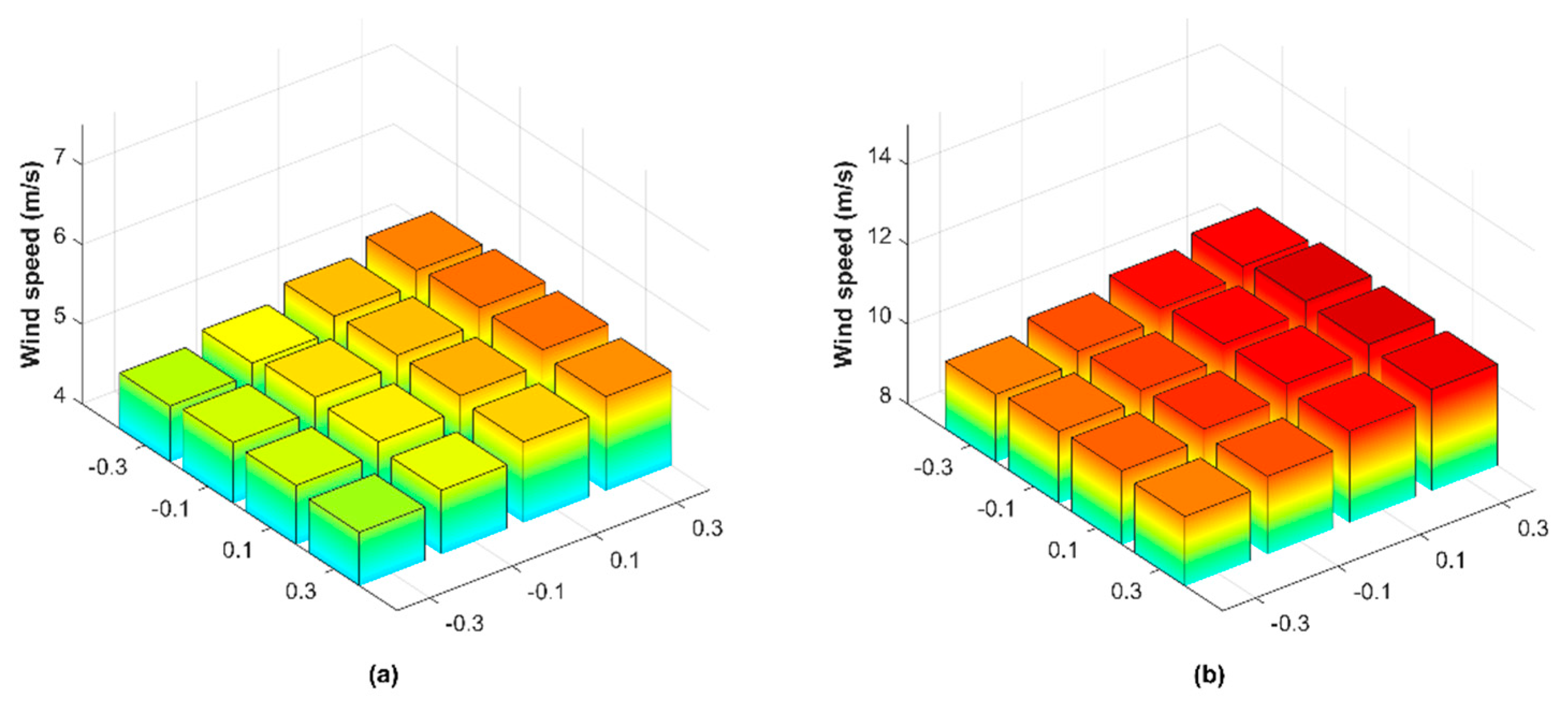
4.2. Discussion of Numerical and Measured Results

For the purpose of investigating the impact caused by varied supply voltage and wind speed, the voltage applied on the conductor is adjusted to −80 kV, −100 kV, and −120 kV, the wind speed is specified at 0 m/s, 5 m/s and 10 m/s. Both the numerically resolved and practically measured results of the electric field and the ion current density on the bottom side of the cage are demonstrated in Figure 10. It shows that the numerical result fits well with that is measured in experiment. As a result, the method used in this work is qualified to evaluate the ion flow field in a corona cage.

The electric field and ion flow current reach their peaks right under the conductor and decrease with the distance from the center point when the wind speed is zero. As the wind speed rises, the curve shifts in the same direction with the wind flow. In comparison with the electric field, the degree of the shift on the ion current density is larger because it is more affected by the movement of the space charges.

In order to illustrate in a more intuitive manner, the cross-section of interest is bisected by vertical center line which is illustrated in Figure 11, the section in where the wind flow and the electric field move in opposite directions is defined as upwind; on the contrary, the other section is downwind.

In the upwind section, electric field and ion current density weakens because the wind flow reduces the density of space charges. This effect decreases as approaching the conductor due to the increasing electric field force.

For both electric field and ion current density, absolute values in the upwind section is slightly lower than that in the downwind section. The absolute value declines along with the increasement of wind speed. In addition, the degree of the impact results from wind speed mounts as the electric field strength decreases. Additionally, the ion current density on lower voltage level is more sensitive to the wind speed owing to weaker field strength.

In upwind and downwind section, the wind flow exerts contrarily influence on the electric field and the ion flow current. To be explicit, increased wind speed weakens the electric field intensity and ion current density in the upwind section. For the downwind section, the result is opposite. The explanation is that the charge density in the upwind section is larger than that of the downwind section which is rather obvious, as shown in Figure 5.

5. Conclusions

The method combining CSM and upwind FVM, which concerns the impact of wind flow, is proposed in this paper, experiment is designed to examine the numeric results. The results indicate that such a method provides a relatively accurate evaluation of the ion flow field under a corona discharge conductor. For the merits of the presented method, the analytically calculated electric field offers a more precise electric field in the vicinity of the conductor than that is solved in traditional FEM; simultaneously, it reduces calculation time and enhances numerical stability to a large extent by means of avoiding iterative calculation of two numeric methods. Moreover, 2nd-order UFVM improves the accuracy of space charge density and is competent for the conditions, including wind impact. The solution process converges effectively and stably. The dependence of the ion flow field on the wind is studied, which approves the influence of wind flow on the ion flow field.

References

1. Maruvada, P.S. Corona Performance of High-Voltage Transmission Lines; Research Studies Press Baldock: Herfordshire, UK, 2000. [Google Scholar]
2. Janischewskyj, W.; Cela, G. Finite Element Solution for Electric Fields of Coronating DC Transmission Lines. IEEE Trans. Power Appar. Syst. 1979, PAS-98, 1000–1012. [Google Scholar] [CrossRef]
3. Takuma, T.; Ikeda, T.; Kawamoto, T. Calculation of ION Flow Fields of HVDC Transmission Lines By the Finite Element Method. IEEE Trans. Power Appar. Syst. 1981, PAS-100, 4802–4810. [Google Scholar] [CrossRef]
4. Abdel-Salam, M.; Farghally, M.; Abdel-Sattar, S. Finite element solution of monopolar corona equation. IEEE Trans. Electr. Insul. 1983, EI-18, 110–119. [Google Scholar] [CrossRef]
5. Li, X.; Ciric, I.R.; Raghuveer, M.R. Highly stable finite volume based relaxation iterative algorithm for solution of DC line ionized fields in the presence of wind. Int. J. Numer. Model. Electron. Netw. Devices Fields 1997, 10, 355–370. [Google Scholar] [CrossRef]
6. Davis, J.L.; Hoburg, J.F. HVDC transmission line computations using finite element and characteristics method. J. Electrost. 1986, 18, 1–22. [Google Scholar] [CrossRef]
7. Fortin, S.; Zhao, H.; Ma, J.; Member, S.; Dawalibi, F.P. A New Approach to Calculate the Ionized Field Transmission Lines in the Space and on the Earth Surface. In Proceedings of the 2006 International Conference on Power System Technology, Chongqing, China, 22–26 October 2006. [Google Scholar]
8. Zhou, X.; Cui, X.; Lu, T.; Fang, C.; Zhen, Y. Spatial distribution of ion current around HVDC bundle conductors. IEEE Trans. Power Deliv. 2012, 27, 380–390. [Google Scholar] [CrossRef]
9. Guillod, T.; Pfeiffer, M.; Franck, C.M. Improved coupled ion-flow field calculation method for AC/DC hybrid overhead power lines. IEEE Trans. Power Deliv. 2014, 29, 2493–2501. [Google Scholar] [CrossRef]
10. Zhang, B.; Mo, J.; He, J.; Zhuang, C. A Time-domain Approach of Ion Flow Field around AC-DC hybrid Transmission Lines Based on Method of Characteristics. IEEE Trans. Magn. 2015, 52, 7205004. [Google Scholar] [CrossRef]
11. Lu, T.; Feng, H.; Cui, X.; Zhao, Z.; Li, L. Analysis of the ionized field under HVDC transmission lines in the presence of wind based on upstream finite element method. IEEE Trans. Magn. 2010, 46, 2939–2942. [Google Scholar] [CrossRef]
12. Zhou, X.; Lu, T.; Cui, X.; Zhen, Y.; Liu, G. Simulation of ion-flow field using fully coupled upwind finite-element method. IEEE Trans. Power Deliv. 2012, 27, 1574–1582. [Google Scholar] [CrossRef]
13. Levin, P.L.; Hoburg, J.F. Donor Cell-Finite Element Descriptions of Wire-Duct Precipitator Fields, Charges, and Efficiencies. IEEE Trans. Ind. Appl. 1990, 26, 662–670. [Google Scholar] [CrossRef]
14. Zhang, B.; He, J.; Zeng, R.; Gu, S.; Cao, L. Calculation of Ion Flow Field Under HVdc Bipolar Transmission Lines by Integral Equation Method. IEEE Trans. Magn. 2007, 43, 1237–1240. [Google Scholar] [CrossRef]
15. Long, Z.; Yao, Q.; Song, Q.; Li, S. A second-order accurate finite volume method for the computation of electrical conditions inside a wire-plate electrostatic precipitator on unstructured meshes. J. Electrost. 2009, 67, 597–604. [Google Scholar] [CrossRef]
16. Yin, H.; He, J.; Zhang, B.; Zeng, R. Finite volume-based approach for the hybrid ion-flow field of UHVAC and UHVDC transmission lines in parallel. IEEE Trans. Power Deliv. 2011, 26, 2809–2820. [Google Scholar] [CrossRef]
17. Yin, H.; Zhang, B.; He, J.; Zeng, R.; Li, R. Time-domain finite volume method for ion-flow field analysis of bipolar high-voltage direct current transmission lines. IET Gener. Transm. Distrib. 2012, 6, 785–791. [Google Scholar] [CrossRef]
18. Yang, F.; Liu, Z.; Luo, H.; Liu, X.; He, W. Calculation of ionized field of HVDC transmission lines by the meshless method. IEEE Trans. Magn. 2014, 50, 7200406. [Google Scholar] [CrossRef]
19. Bian, X.; Yu, D.; Meng, X.; Macalpine, M.; Wang, L.; Guan, Z.; Yao, W.; Zhao, S. Corona-generated space charge effects on electric field distribution for an indoor corona cage and a monopolar test line. IEEE Trans. Dielectr. Electr. Insul. 2011, 18, 1767–1778. [Google Scholar] [CrossRef]
20. Lekganyane, M.J.; Ijumba, N.M.; Britten, A.C. A comparative study of space charge effects on corona current using an indoor corona cage and a monopolar test line. In Proceedings of the 2007 IEEE Power Engineering Society Conference and Exposition in Africa, Johannesburg, South Africa, 16–20 July 2007. [Google Scholar]
21. Kaptzov, N.A. Elektrische Vorgänge in Gasen und im Vakuum; VEB Deutscher Verlag der Wissenschaften: Berlin, Germany, 1955; pp. 488–491. ISBN 978-3-446-42771-6. [Google Scholar]
22. Peek, F.W. Dielectric Phenomena in High Voltage Engineering; McGraw-Hill Book Company, Inc: New York, NY, USA, 1920. [Google Scholar]
23. Abdel-salam, M.; Al-hamouz, Z. A finite-element analysis of bipolar ionized field. IEEE Tans. Ind. Appl. 1995, 31, 477–483. [Google Scholar] [CrossRef]
24. Zhou, X.; Cui, X.; Lu, T.; Zhen, Y.; Luo, Z. A time-efficient method for the simulation of ion flow field of the AC-DC hybrid transmission lines. IEEE Trans. Magn. 2012, 48, 731–734. [Google Scholar] [CrossRef]
25. Li, X. Numerical Analysis of Ionized Fields Associated with HVDC Transmission Lines Including Effect of Wind. Ph.D. Thesis, The University of Manitoba, Winnipeg, MB, USA, 1997. [Google Scholar]
26. Urban, R.G.; Reader, H.C.; Holtzhausen, J.P. Small corona cage for wideband HVac radio noise studies: Rationale and critical design. IEEE Trans. Power Deliv. 2008, 23, 1150–1157. [Google Scholar] [CrossRef]
Figure 1. Flowchart of the method.
Energies 12 03924 g001
Figure 2. Tessellation of calculation domain.
Energies 12 03924 g002
Figure 3. CSM method.
Energies 12 03924 g003
Figure 4. Control volume of UFVM.
Energies 12 03924 g004
Figure 5. Space charge density under 100 kV supply voltage. (a) space charge density under 0 m/s wind speed; (b) space charge density under 5 m/s wind speed; and (c) space charge density under 10 m/s wind speed.
Energies 12 03924 g005
Figure 6. Convergence to terminal criteria.
Energies 12 03924 g006
Figure 7. Schematic diagram of the experimental setting.
Energies 12 03924 g007
Figure 8. (a) The general view of the corona cage; (b) The electric field mill; (c) The Wilson plate; (d) Flow equalizing plate; (e) adjustable speed fan; (f) digital high precision anemometer; and (g) scope coder.
Energies 12 03924 g008
Figure 9. (a) measured wind speeds of 5 m/s; and (b) measured wind speeds of 5 m/s.
Energies 12 03924 g009
Figure 10. (a) Electric field on the bottom side under −80 kV supply voltage; (b) electric field on the bottom side under −100 kV supply voltage; (c) electric field on the bottom side under −120 kV supply voltage; (d) ion current density on the bottom side under 80 kV supply voltage; (e) ion current density on the bottom side under 100 kV supply voltage; (f) ion current density on the bottom side under 120 kV supply voltage.
Energies 12 03924 g010
Figure 11. Schematic diagram of the cross-section.
Energies 12 03924 g011