Abstract
A simple effective model is proposed for the day-ahead electricity market. The model considers the main factors which govern the process, predicts the seasonal and daily variation of electricity demand, renewable production, system marginal price, and merit order effect. The accuracy of the model is increased by fitting to historic data of the Hellenic electricity market. During the period between October 2016 and December 2018, the Hellenic electricity market calculated explicitly the merit order effect using an innovative mechanism to directly charge the electricity suppliers (retailers). On the basis of the proposed model and the market recorded data, the effect of the renewable penetration on the wholesale Hellenic electricity prices is revealed. The model is further used to analyze the market future behavior when basic factors (electricity demand, conventional power, and renewable penetration) are known or estimated. The effect of merit order effect on the Hellenic legislation is discussed and the appropriate measures adopted by the Hellenic authorities are analyzed and evaluated.
1. Introduction
The integration of renewable energy sources (RES) in electricity markets has been significantly reinforced by policy support measures in all European countries. The effect of their participation on the determination of electricity wholesale marginal prices has become, however, a topic of political debate. Considering that renewables enter with priority into the day-ahead market (DAM) (zero pricing bids), the merit order curve (MOC) is shifted to the right or equivalent, the demand curve is shifted to the left, most expensive plants are driven out, and subsequently, the clearing wholesale marginal electricity price is diminished. This phenomenon is the so-called merit order effect (MOE). Since intense discussions have taken place about the economic surcharge that passes to the final consumers due to renewable supporting mechanisms, a broad spectrum of literature exists on the analysis, quantification, and evaluation of the MOE phenomenon.
The methods for the examination of MOE are based on two main approaches [1,2], which are as follows: (a) the development of electricity market models, which simulate the operation of DAM and calculate the resulted spot electricity price for various scenarios [3,4,5,6,7,8,9] and (b) the regression analysis approach, which uses historical price and generation data in order to quantify the actual achieved reduction in spot price for a given period of time [2,3,10,11,12,13,14]. Studies that combine both approaches are also met [15]. Although each country has its unique characteristics in terms of energy mix, economic growth, incentives policy, etc., useful information and knowledge can be retrieved by relevant research.
The impact of the RES generation in Germany was analyzed by Sensfuß et al. [8], by developing a detailed electricity market simulation model. The results showed the high impact of the diffusion of renewables on spot market prices, reaching a reduction of 7.8€/MWh (2006). For the same country, Weigt [6] investigated the impact of wind penetration, and indicated a significant decline in market price, especially during peak periods (10€/MWh). In Spain, two relevant studies were found in the literature. De Miera [7] assessed the effect of support schemes on power prices for the case of wind-generation electricity, and concluded that the reduction of spot price was much higher than the increase in cost charged to the consumers for the financial support of the technology. Ciarreta et al. [9] analyzed the Spanish electricity market for four years (2008–2012) and calculated the cost of “green” energy as the difference between the savings gained due to MOE and the incentive amounts. According to the results, after the wide deployment of RES, a positive net cost was computed, but a difference in the cost among technologies was observed.
The significant impact of wind generation on spot prices was also proven by Jónsson et al. [11], who used a non-parametric regression model to analyze the Danish electricity market. Similarly, based on the regression approach, Luňáčková et al. [14] quantified the MOE in the Czech market by using six years of hourly, daily, and weekly data (2010–2015), which led to the outcome of a 10% increase in RES deployment, except from solar which had a negative impact in general, and caused a 2.5% decrease in electricity price. Gelabert et al. [10] used a multivariate regression model to estimate the MOE of the RES and cogeneration in Spain between 2005 and 2010 and showed that a marginal increase of 1 GWh of electricity production from the previous technologies leads to a decrease of 2€/MWh in electricity prices. In the case of Italy, Clò et al. [3] used empirical data from the DAM and proved that wholesale electricity prices were reduced by 2.3€/MWh and 4.2€/MWh due to an increase of 1 GWh in the hourly average of daily produced energy from solar and wind systems, respectively.
In Greece, the share of RES in electricity production mixture increased from to 6.9% in 2004 to 16.3% in 2017, while the national target for 2020 is 18% [16]. The main incentive for the RES wide penetration in the country has been the feed-in tariff (FIT) mechanism [17,18]. The impact of this deployment on the Hellenic electricity market was evaluated by Simoglou et al. [19,20], by developing a simulation model for the market operation under various scenarios of RES capacity. The results indicated that RES integration caused a significant reduction in the SMP (system marginal price) and CO2 emissions, but the payment of consumers was increased for the examined years (2009 and 2011).
This paper aims to extend the current literature and quantify, as well as analyze the MOE in the Hellenic wholesale electricity DAM by: (1) analyzing historic data, (2) proposing and validating a simple model describing the phenomenon, (3) analyzing future market behavior when the crucial factors are known or predicted, and (4) analyzing and evaluating the related surcharge mechanism used by the Hellenic authorities. The MOE analysis refers to seasonal and daily variation of the MOE along with the effect of renewable technology on the MOE. The political significance of MOE in electricity pricing along with the Hellenic authorities curing experiment (2016–2018) are analyzed in Section 2, and the corresponding recording data are statistically analyzed in Section 4.1. A robust mathematical model is proposed in Section 3, which is fitted to recording data in Section 4.2 and used to analyze future market behavior in Section 4.3. Section 5 summarizes the conclusions of the analysis.
2. Merit Order Effect and the Hellenic Electricity Market
Greece enjoys a renewable energy sources (RES) installed capacity of approximately 5 GW operating under the feed-in tariff (FIT) model, initially introduced by law 3468/2006 [21]. Priority to the grid applies also to net-metering, virtual net-metering, and feed in premium scheme lastly introduced through law 4414/2016 [22] leading, as well, to a further decline of the system marginal price (SMP).
The RES account introduced through law 2773/1999 [23], is responsible for payments of renewable electricity production under feed-in supporting schemes. Its revenue architecture faced significant challenges and deficits in Greece during the last decade, leading the RES investments all over the country to payment delays, financial problems, and unfortunately retroactive cuts in contracted tariffs even for operating projects through laws 4093/2012 [24], 4152/2013 [25], and finally 4254/2014 [26]. Although at first sight one could claim that the RES account deficits were solely driven by rapid expansion of renewables during 2011 to 2013 without a simultaneous and adequate increase in the RES levy (called ETMEAR in Greece) in consumer electricity bills, the continuation of financial problems of the RES account even after retroactive cuts in tariffs of 2012–2014, indicated the problematic revenue architecture of the account.
Focusing closer on the RES account structure [27], a major revenue component has to do with its income from the wholesale market, corresponding to the renewable electricity produced and infused into the grid multiplied by the hourly SMP. In order to provide priority for renewables to the grid over other conventional sources such as lignite or gas-fired plants or imports, feed-in operating models (feed-in tariff or feed in premium) provide that RES are not truly participating in the wholesale market with price bids that compete with fossil fuel bids but instead their bidding price remains zero every hour in order to be always preferable and selected to feed-in [28].
Therefore, regardless of the specific operating model, such as FIT, FIP, or net-metering, it is the priority in entering the market (grid) that renewable energy enjoys through zero bidding prices that diminishes SMP in DAM and, consequently, RES account revenues for renewable overall electricity production infused. This naturally means that a further increase in renewable capacity under priority, even at comparable to SMP price levels, is expected to expand MOE further, diminishing SMP even more and consequently further triggering the need for a RES levy increase, in order for the RES account to keep its financial ability to support contracted prices for renewables. This systematic decline of SMP due to RES priority is benefiting suppliers not only for the renewable electricity they buy at this lower marginal wholesale market price but for all their electricity needs drawn from the pool, because for each hour the wholesale price is one and unique [29].
On the one hand, the RES levy not only works to finance the true cost difference between renewable and fossil fuel electricity, but as a tool to cover the continuously increasing distortion because of MOE and the missing money problem it causes for the RES account [29]. It is obvious that a general withdrawal of RES as a priority aiming to minimize MOE and hence the RES account distortion in revenues through SMP, could not be part of a viable solution. The stochastic nature of wind and solar energy production could cause them to not survive direct competition against fossil fuels, unless storage solutions become reliable and economically effective for them.
On the other hand, one could argue that for the consumer the distortion of MOE finally plays no role regarding total electricity bill cost, since the increased RES levy is counteracted by the reduced wholesale electricity cost based on the diminished SMP. In other words, the added amount of money that the regulated part of the bill (through RES levy) needs to carry because of the distortion of MOE, is balanced by the decrease in the nonregulated or so called “competitive” part of the bill. Furthermore, if new renewables entering the system are remunerated with tariffs close to the SMP levels, as it now happens, then electricity bills for the consumer will no longer increase. However, even new renewables, because of their priority entrance under zero pricing bidding, will trigger a further SMP decline and need for a RES levy increase not only for them but for all other previously existing and operating RES penetration, and hence the vicious circle continues even more aggressively.
Real life in Greece during the recession years showed that regulated electricity costs bare political costs, meaning that authorities are, in general, reluctant or negative towards increasing a part of the electricity bill, especially when they cannot easily explain to consumers why this is happening (MOE is difficult to describe) and at the same time when they cannot directly control the nonregulated part of the bill that should be equally decreased.
During 2015, the RES account in Greece started showing deficits again due to a SMP drop. Suppliers did not proceed to electricity price reductions in the competitive part but instead kept high profitability margins benefiting from the MOE in order to face the growing phenomenon of unpaid consumer bills. At the same time, the RES levy was officially frozen against increases by the State. Less than a year later, during 2016, delays in payments for renewables, due to the RES account increasing cumulative deficit, started to rapidly rise jeopardizing national policies against climate change and of course Greece’s credibility as an investment destination. Therefore, public dialogue and the challenge during that time was to determine how to take out of the RES levy its distorted part due to the MOE and charge it to suppliers that were systematically benefitting from high margins out of it.
Towards this aim, the idea was to introduce a parallel virtual wholesale market being resolved every hour exactly as the official one but excluding renewables that operate under priority. Out of this virtual market, a virtual SMP could be calculated and its difference from the official SMP would give the decline of the SMP because of MOE. This difference between the virtual SMP (VSMP) and the official one multiplied by the amount of MWh each supplier drew from the pool in order to cover the demand of its customers, would represent a new charge for suppliers. This new charge, domestically called “PXEFEL”, aimed to make suppliers return to the RES account their systematic economic benefit and increased margin because of the RES and the MOE they caused.
In this respect, by having the RES account as an additional regular revenue through the MOE charge counteracting the MOE, the RES levy could be kept to the necessary, fair (not distorted) lower levels. The aim of the RES levy was to make it correspond to whatever difference in the production costs truly exists between fossil and renewable sources. On the other hand, for suppliers, the MOE charge consisted of a new cost component incorporated into the “competitive” part of their consumer bills, whereby suppliers had the ability to disperse it in a variety of manners among different customer groups in correlation to their hourly consuming profile. The MOE differs significantly among different hours in the DAM, since it mainly has to do with electricity demand and RES active penetration.
A radical alternative solution proposed at that time was to fully integrate the RES levy into the wholesale cost of suppliers, and hence to the “competitive” part of their bills. To do so, the market operator would have to charge them a “below the line” RES levy on the basis of electricity drawn from the DAM pool. Suppliers would then fully incorporate the cost of the RES levy in their pricing policies, mixed of course with their benefit from the MOE that the RES at the same time cause. Suppliers’ bills would then become more market oriented, since there would be no regulated part for the RES electricity cost that suppliers do not “own”. This model would be somehow equivalent to suppliers being contracted directly by the RES producers through bilateral contracts to purchase their production at their fixed tariffs.
3. Day-Ahead Electricity Market Model
The proposed mathematical model aims to predict the MOE versus the crucial factors affecting the DAM. It is basically a deterministic model which considers the “predictable” part of the seasonal and daily variation of the demand and renewable production, while the “random” part is considered as just a noise which is eliminated by fitting to historical data. Random variation could be considered by adding random functions describing the noise, but this is out of the scope of the present paper. A stochastic model for probabilistic forecasting has been proposed recently by Bello et al. [30].
3.1. Definition of the Merit Order Effect
Mathematically, the MOE is defined as the difference in system marginal price between (a) the value calculated when all the demand is considered into market clearance procedure, the virtual system marginal price (VSMP) and (b) the value calculated when the renewable production is excluded from the demand, the system marginal price (SMP). That is, MOE = VSMP − SMP.
This definition is graphically presented in Figure 1.
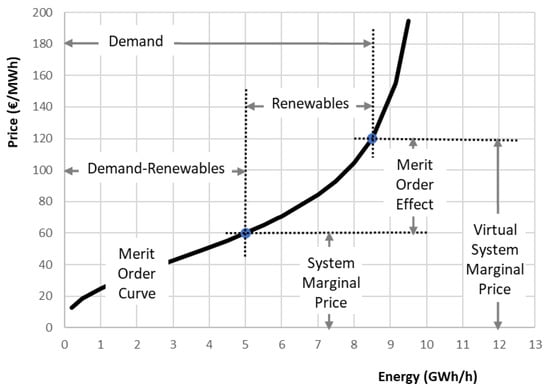
Figure 1.
Definition of the merit order effect (MOE) using the demand and supply curve (merit order curve) in the day-ahead electricity market.
3.2. The Merit Order Curve
The supply curve in the DAM is called the merit order curve (MOC). The following equation is proposed and used in this paper to describe it:
where the supply price (€/MWh) is calculated versus the dispatchable electricity supply (GWh/h), when the following three parameters are known:
- GWh/h the maximum feasible electricity supply;
- €/MWh the electricity price at half of maximum supply;
- - empirical shape constant.
Obviously, the maximum feasible electricity supply is analogous to the conventional installed power (lignite-fired, gas-fired, and large hydro) that are dispatchable, meaning that they have the ability to determine the SMP through their hourly price bidding in the DAM.
The above analysis assumes that other factors affecting the MOC remain constant during the analysis period. Other factors such as the suppliers bidding strategy, the CO2 emissions price, and the fuel price can be introduced in the parameters and through appropriate functions, but this is out of the scope of this paper.
3.3. The Electricity Demand
The electricity demand appears to have both seasonal and daily variations. The seasonal variation of the electricity demand appears as two peaks, one during the winter and one during the summer. Loumakis et al. [31] considered the following three additive kinds of demand with different variation each: (a) A constant demand independently of the season, (b) a winter activities demand, and (c) a summer activities demand. A normal distribution was proposed to describe both the winter and summer activities with different characteristics. The resulting equation is [31]:
where the electricity demand (GWh/day) during the day i (1, 2, …, 365) is calculated, when the following seven parameters are known:
- GWh/year the total electricity demand during the year;
- - the portion of the total annual demand for winter activities;
- - the portion of the total annual demand for summer activities;
- days the time of the peak of winter activities;
- days the time of the peak of summer activities;
- days the typical duration of the winter activities;
- days the typical duration of the summer activities.
The normal distribution is expressed by the following equation: .
The daily variation of the demand also appears to have two peaks, one at noon and another in the evening. The above idea concerning the seasonal variation is also used to describe the daily variation:
where the electricity demand (GWh/hour) during the hour j (= 1, 2, …, 24) of the day i (1, 2, …, 365) is calculated, when the total demand (GWh/day) of the day i is calculated from Equation (2) and the following six parameters are additionally known:
- - the portion of the total daily demand for noon activities;
- - the portion of the total daily demand for evening activities;
- hours the time of the peak of noon activities;
- hours the time of the peak of evening activities;
- hours the typical duration of the noon activities;
- hours the typical duration of the evening activities.
3.4. Renewable Electricity Production
The renewable electricity production appears also to have both seasonal and daily variations. Loumakis et al. [31] proved that all types of renewables follow a cosine seasonal variation with different amplitude and peak time. Thus, the resulting total renewable also appears cosine variation with characteristics depended on renewable mixture. Instead, concerning daily variation, all renewables, except photovoltaics, are random or almost constant without any deterministic variation. Photovoltaics follows a well-known deterministic variation during daytime sunshine hours. On the basis of these remarks the renewables can be divided into two categories, concerning the daily variation profile, the photovoltaics (PV), and the other (W). Thus:
where:
- i days the day of the year (1, 2, …, 365);
- GWh/day the electricity generated from renewables during the day i;
- GWh/day the electricity generated from renewables except photovoltaics during the day i;
- GWh/day the electricity generated from photovoltaics during the day i.
The seasonal variation of both kinds of renewables is described by the cosine equation:
Equation (5) calculates the electricity (GWh/day) generated from renewables except photovoltaics during the day of the year i (1, 2, …, 365), when the following three parameters are known:
- GWh/year the total annual electricity generated by renewables except photovoltaics;
- GWh/day the seasonal variation amplitude of renewables except photovoltaics;
- days the day of minimum production for renewables except photovoltaics.
Equation (6) calculates the electricity (GWh/day) generated from photovoltaics during the day of the year i (1, 2, …, 365), when the following three parameters are known:
- GWh/year the total annual electricity generated by photovoltaics;
- GWh/day the seasonal variation amplitude of photovoltaics;
- days the day with the minimum production for photovoltaics.
Concerning the daily variation, the following equations are proposed:
Equation (7) calculates the electricity (GWh/hour) generated from renewables except photovoltaics during the hour j (1, 2, …, 24) of the day of the year i (1, 2, …, 365), when the total daily electricity is calculated by Equation (5) (uniform distribution).
Equation (8) calculates the electricity (GWh/hour) generated from photovoltaics during the hour j (1, 2, …, 24) of the day i (1, 2, …, 365), when the total daily electricity is calculated by Equation (6) and the following parameter is additionally known:
- hours the hour with maximum production from photovoltaics.
The correction factor cf is given by the equation:
3.5. Regression Analysis
The resulting mathematical model of Equations (1)–(8) calculates all crucial quantities of the electricity market (electricity demand, renewable generation, merit order curve, system marginal price, and merit order effect) when twenty-three parameters are known. The information flow diagram of the proposed model is presented in Figure 2.
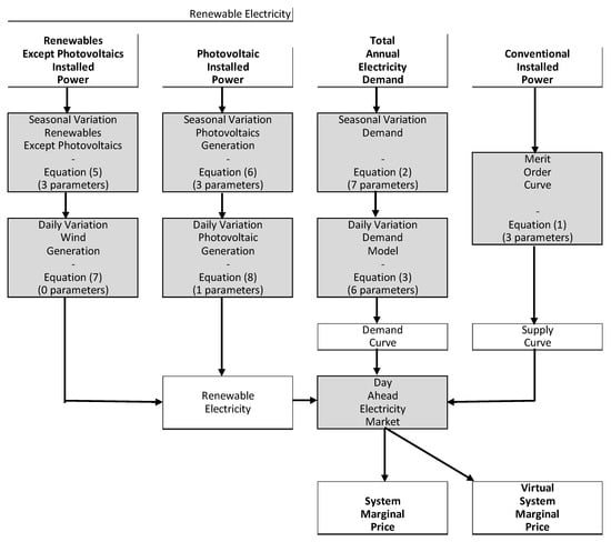
Figure 2.
Model information flow diagram.
The parameters can be estimated using three separate regressions:
- Equations (2) and (3) are simultaneous fitted to real data of demand;
- Equations (5)–(8) are simultaneous fitted to real data of renewable electricity generation;
- Equation (1) is fitted to real data of system marginal price and virtual marginal price.
The appropriate data were retrieved from the Hellenic electricity market operator [32] and the Hellenic energy exchange group [33].
During the period from October 2016 to December 2018 (27 months) the auction clearing process of the DAM was calculated twice (a) using the demand and supply including renewables in order to obtain the system marginal price (SMP) and (b) using the demand and supply excluding renewables in order to obtain the corresponding SMP without the renewables, denoted as virtual system marginal price (VSMP).
The following data were retrieved for the whole year 2017:
- GWh/h Hourly electricity demand;
- GWh/h Hourly renewables electricity;
- €/MWh Hourly system marginal price;
- €/MWh Hourly virtual system marginal price.
where i is the day identification number (1, 2, …, 365) and j the hour identification number (1, 2, …, 24) per day.
The resulting fitted model can be used to forecast by changing the following parameters (factors):
- GWh/h the maximum feasible electricity supply;
- GWh/year the total annual electricity generated by renewables except photovoltaics;
- GWh/year the total annual electricity generated by photovoltaics;
- GWh/year the total electricity demand during the year.
All other model parameters cannot be considered as factors since they remain long-term constants. They are not analogous to the market size, but they are dependent on the country activities and weather characteristics.
4. Results and Discussion
4.1. Statistical Analysis
The recording quantities (D, R, VSMP, and SMP) along with the calculated ones (DR = D − R and MOE = VSMP − SMP) are presented in Figure 3. Hourly data are plotted, that is 8760 points for each quantity. The time duration curves are also presented in Figure 3. Furthermore, the basic statistics are presented in Table 1 and the corresponding fitted normal distributions in Figure 4.
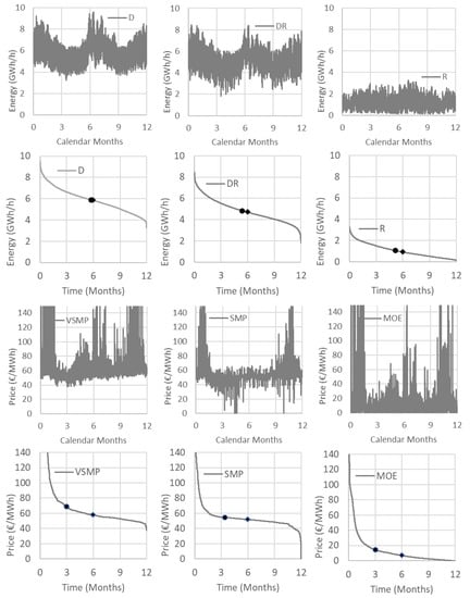
Figure 3.
Real data versus time along with the corresponding duration curves: D = demand, DR = demand renewables, R = renewables, VSMP = virtual system marginal price, SMP = system marginal price, MOE = merit order effect. Data from Hellenic electricity market operator [32] and the Hellenic energy exchange group [33].

Table 1.
Basic statistics.
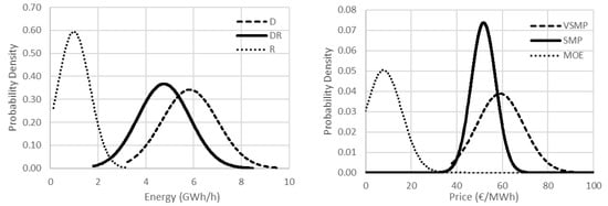
Figure 4.
Fitted normal distribution: D = demand, DR = demand renewables, R = renewables, VSMP = virtual system marginal price, SMP = system marginal price, MOE = merit order effect.
The examined quantities, as analyzed in the previous sections, appear as seasonal and daily variation. Seasonal variation is revealed using 24 h moving averages which eliminate the daily variation. The results are presented in Figure 5.
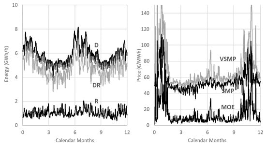
Figure 5.
Seasonal variation using 24 hour moving averages: D = demand, DR = demand renewables, R = renewables, VSMP = virtual system marginal price, SMP = system marginal price, MOE = merit order effect.
Daily variation is revealed by averaging data separately for each hour of the day. Averaging is performing for every month since due to seasonal variation every month different daily characteristics appear. The results are presented in Figure 6 and Figure 7.
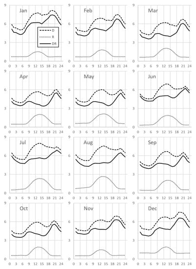
Figure 6.
Daily variation using monthly-averaged hourly data: D = demand, DR = demand renewables, R = renewables. Horizontal axis = hour of the day, vertical axis = energy in GWh/h.
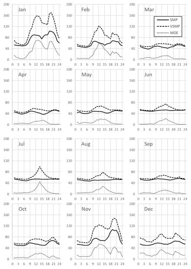
Figure 7.
Daily variation using monthly-averaged hourly data: VSMP = virtual system marginal price, SMP = system marginal price, MOE = merit order effect. Horizontal axis = hour of the day, vertical axis = price in €/MWh.
It must be noticed that, during January and July 2017, peak demand conditions were met resulting, as expected, in higher SMP, VSMP prices, and MOE.
Due to the pan-European electricity crisis triggered by the withdrawal of several nucleal plants in France for service and repair reasons in late Autumn 2016, wholesale electricity prices all over Europe climbed to very high levels during December 2016 to January 2017. To cover the gap, France turned to imports of electricity from neighbour countries dispersing crisis all over Europe. The extra needs for electricity were covered mostly from natural gas-fired plants leading to a gas market crisis as well. This climb also happened with the SMP in Greece and of course the VSMP. Winter peaking demand reinforced, as expected, market thirst and anxiety for electricity. In February of 2017, the Regulatory Authority of Energy (RAE) imposed a ceiling of 15€/MWh per hour for MOE in order to avoid its extreme values leading to excessive burden for suppliers. The same electricity demand anxiety phenomenon occurred also at the end of 2017 mostly due to bad cold weather conditions reinforced by the memory and fear of the previous year’s crisis as well.
Two electricity demand peaks per day are observed in Figure 6, one during noon and the second in the evening. Noon peak demand is almost completely covered by the PV production all over the year. Noon peak is higher compared to evening peak during summer months while the contrary happens in winter.
Figure 7 shows how the SMP prices escalate when electricity demand is peaking and what happens to wholesale prices (VSMP) if the RES were not present. Furthermore, the PV penetration leads to time concentrated electricity production during noon hours and reduces the SMP during these hours at the most, resulting in the highest MOE values.
4.2. Regression Analysis
Table 2 presents the parameter estimates from the regression analysis as described in the previous sections. Three different regressions were applied and the comparison between real and calculated values are presented in Figure 8, Figure 9, Figure 10 and Figure 11.
Table 2.
Model parameter estimation results.
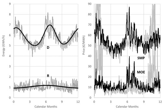
Figure 8.
Seasonal variation: Comparison between real (grey lines) and model calculated (black lines) values. D = demand, R = renewables, SMP = system marginal price, MOE = merit order effect.
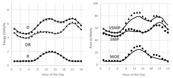
Figure 9.
Daily variation: Comparison between real (points) and model calculated (lines) values. D = demand, DR = demand renewables, R = renewables, VSMP = virtual system marginal price, SMP = system marginal price, MOE = merit order effect.
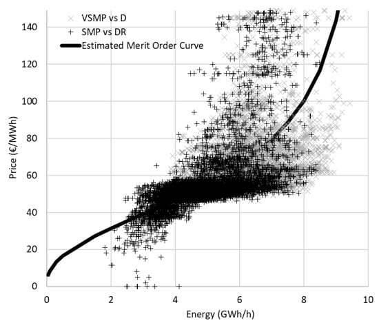
Figure 10.
Merit order curve: Comparison between real and model calculated values.
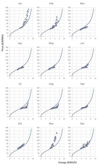
Figure 11.
Merit order curve: Comparison between real and model calculated values. Monthly averaged values.
Parameters in Table 2 express either (a) the market characteristics (weather, demand, generation technologies, etc) which remain constant long term or (b) the market size (demand, conventional and renewable installed power, etc) which follow the growth of economy.
The four parameters which express the market size are:
- GWh/h the maximum feasible electricity supply;
- GWh/year the total annual electricity generated by renewables except photovoltaics;
- GWh/year the total annual electricity generated by photovoltaics;
- GWh/year the total electricity demand during the year.
is analogous to the installed power of conventional electricity generated systems that are dispatchable, meaning that they determine SMP through hourly price bidding in the day-ahead market. Similarly, and are analogous to the renewable installed power, non-photovoltaics and photovoltaics, respectively. Finally, expresses the society activities and is analogous to the economic growth.
Thus, it is useful to compare the estimated values of these parameters with the recorded values:
- Estimated values of and are exactly as recorded 51.9 TWh/y and 3.72 TWh/y, respectively, while estimated value of is a little higher than recorded 5.84 TWh/y;
- Smax of 9.88 GWh/h is a decline from the expected installed conventional power of 12 GW, because the total capacity does not participate continuously into the market.
4.3. Sensitivity Analysis
The proposed mathematical model can be used to predict electricity market behavior in the future when the parameter estimates in the Table 2 are adjusted to future values. The four parameters which express the size of the market are considered as factors. All other parameters express market characteristics which remain constant long term. Thus, the factors which affect market future behavior are the following four parameters:
- GWh/h the maximum feasible electricity supply;
- GWh/year the total annual electricity generated by renewables except photovoltaics;
- GWh/year the total annual electricity generated by photovoltaics;
- GWh/year the total electricity demand during the year.
is analogous to the installed power of conventional electricity generated systems that are dispatchable, meaning that they determine SMP through hourly price bidding in the day-ahead market. Similarly, and are analogous to the renewable installed power, non-photovoltaics and photovoltaics, respectively. Finally, expresses the society activities and is analogous to the economic growth.
In the sensitivity analysis of Figure 12 the effect of the above four factors on the merit order effect (MOE), separately, is presented. Demand is the crucial factor; it can double the MOE when it increases by about 25%. Renewables appear to have a smaller effect, while conventional installed power appears to have a negative effect. Obviously, all these effects are interpreted from Figure 1 by changing the interception of the demand and supply curves.
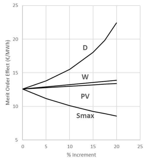
Figure 12.
Sensitivity analysis (one factor at a time): Effect of crucial market factors on the merit order effect. D = demand, W = renewables except photovoltaics, PV = photovoltaics, and Smax = conventional.
The effect of the factors when they are changed simultaneously is presented in the scenario analysis of Figure 13. The following scenarios are examined:
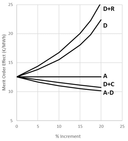
Figure 13.
Scenario analysis (simultaneous factor variation): D + R = demand and renewables are increased by the same rate, conventionals are kept constant; D = demand is increased, all other factors are kept constant; A = all factors are increased by the same rate; D + C = demand and conventionals are increased with the same rate, renewables are kept constant; and A − D = all factors, except demand, are increased by the same rate.
- D Demand is increased, all other factors are kept constant;
- D + R Demand and renewables are increased by the same rate and conventionals are kept constant;
- D + C Demand and conventionals are increased with the same rate and renewables are kept constant;
- A All factors are increased by the same rate;
- A − D All factors except Demand are increased by the same rate.
Obviously, the higher positive effect is obtained when demand and renewables are increased simultaneously, and the higher negative effect is obtained when demand remains constant and all other factors are increased. Similarly, any other combination of changes can be examined.
5. Conclusions
During the period between October 2016 and December 2018 the Hellenic DAM calculated explicitly the MOE using an innovative mechanism to directly charge the electricity suppliers. Through the MOE charge (called PXEFEL in Greeks), suppliers were returning to the RES account the financial benefit they were enjoying because of MOE, namely the lower SMP values in the DAM due to RES penetration.
The above mechanism needs an appropriate model to evaluate and analyze daily, seasonal, and long-term variations of the MOE towards an optimum MOE charge strategy. Thus, a simple model for the DAM is proposed and validated to real data. The model, considering the main factors which govern the process, predicts the seasonal and daily variation of electricity demand, renewable production, SMP, and MOE. The model was fitted adequately to historic data of the Hellenic DAM during the year 2017.
The model innovation is based on the separate direct simulation of the supply and demand curves and the seasonal and daily variation of the electricity demand and renewable generation.
On the basis of the proposed model and the market recorded data, the effect of the renewable penetration on the wholesale electricity prices is analyzed.
The model can further be used to predict future market behavior when the basic factors (electricity demand, conventional power, conventional costs, and renewable penetration) are known or estimated. Thus, the effect of the evolution of the RES penetration on the MOE can be estimated and analyzed towards an optimum RES penetration supporting strategy.
The proposed model was applied successfully to the Hellenic electricity market, but it can be used to any other similar market.
Author Contributions
All authors contributed equally.
Funding
This research received no external funding.
Conflicts of Interest
The authors declare no conflict of interest.
Nomenclature
| the correction factor (-) | |
| the portion of the total daily demand for evening activities (-) | |
| the electricity demand during the day i (GWh/day) | |
| the electricity demand during the hour j of the day i (GWh/hour) | |
| the portion of the total daily demand for noon activities (-) | |
| the portion of the total annual demand for summer activities (-) | |
| the total electricity demand during the year (GWh/year) | |
| the portion of the total annual demand for winter activities (-) | |
| the day of the year (1, 2, …, 365) (days) | |
| the day with the minimum production for photovoltaics (days) | |
| the day of minimum production for renewables except photovoltaics (days) | |
| the hour with maximum production from photovoltaics (hours) | |
| the hour with maximum production from photovoltaics (hours) | |
| empirical shape constant (-) | |
| the supply price (€/MWh) | |
| the electricity generated from photovoltaics during the day i (GWh/day) | |
| the electricity generated from photovoltaics during the hour j of the day i (GWh/hour) | |
| the electricity price at half of maximum supply (€/MWh) | |
| the total annual electricity generated by photovoltaics (GWh/year) | |
| the electricity generated from renewables during the day i (GWh/day) | |
| the electricity generated from renewables during the hour j of the day i (GWh/hour) | |
| the dispatchable electricity supply (GWh/h) | |
| the maximum feasible electricity supply (GWh/h) | |
| the System Marginal Price (€/MWh) | |
| the System Marginal Price during the hour j of the day i (€/MWh) | |
| the time of the peak of evening activities (hours) | |
| the time of the peak of noon activities (hours) | |
| the time of the peak of summer activities (days) | |
| the time of the peak of winter activities (days) | |
| the Virtual System Marginal Price (€/MWh) | |
| the Virtual System Marginal Price during the hour j of the day i (€/MWh) | |
| the electricity generated from renewables except photovoltaics during the day i (GWh/day) | |
| the electricity generated from renewables except photovoltaics during the hour j of the day i (GWh/hour) | |
| the total annual electricity generated by renewables except photovoltaics (GWh/year) | |
| the seasonal variation amplitude of photovoltaics (GWh/day) | |
| the typical duration of the evening activities (hours) | |
| the typical duration of the noon activities (hours) | |
| the typical duration of the summer activities (days) | |
| the typical duration of the winter activities (days) | |
| the seasonal variation amplitude of renewables except photovoltaics (GWh/day) |
Abbreviations
| A | all |
| C | conventionals |
| CO2 | carbon dioxide |
| D | demand |
| DAM | day-ahead market |
| DR | demand minus renewables |
| ETMEAR | surcharge on electricity price (Greek abbreviation) |
| FIP | feed-in premium |
| FIT | feed-in Tariff |
| MOC | merit order curve |
| MOE | merit order effect |
| PVs | photovoltaics |
| PXEFEL | merit order effect charge (Greek abbreviation) |
| R | renewables |
| RAE | regulatory authority of energy |
| RES | renewable energy sources |
| SMP | system marginal price |
| VSMP | virtual system marginal price |
| W | renewables except photovoltaics |
References
- Cludius, J.; Forrest, S.; MacGill, I. Distributional effects of the Australian Renewable Energy Target (RET) through wholesale and retail electricity price impacts. Energy Policy 2014, 71, 40–51. [Google Scholar] [CrossRef]
- Cludius, J.; Hermann, H.; Matthes, F.C.; Graichen, V. The merit order effect of wind and photovoltaic electricity generation in Germany 2008–2016 estimation and distributional implications. Energy Econ. 2014, 44, 302–313. [Google Scholar] [CrossRef]
- Clò, S.; Cataldi, A.; Zoppoli, P. The merit-order effect in the Italian power market: The impact of solar and wind generation on national wholesale electricity prices. Energy Policy 2015, 77, 79–88. [Google Scholar] [CrossRef]
- Traber, T.; Kemfert, C. Gone with the wind? Electricity market prices and incentives to invest in thermal power plants under increasing wind energy supply. Energy Econ. 2011, 33, 249–256. [Google Scholar] [CrossRef]
- McConnell, D.; Hearps, P.; Eales, D.; Sandiford, M.; Dunn, R.; Wright, M.; Bateman, L. Retrospective modeling of the merit-order effect on wholesale electricity prices from distributed photovoltaic generation in the Australian National Electricity Market. Energy Policy 2013, 58, 17–27. [Google Scholar] [CrossRef]
- Weigt, H. Germany’s wind energy: The potential for fossil capacity replacement and cost saving. Appl. Energy 2009, 86, 1857–1863. [Google Scholar] [CrossRef]
- De Miera, G.S.; del Río González, P.; Vizcaíno, I. Analysing the impact of renewable electricity support schemes on power prices: The case of wind electricity in Spain. Energy Policy 2008, 36, 3345–3359. [Google Scholar] [CrossRef]
- Sensfuß, F.; Ragwitz, M.; Genoese, M. The merit-order effect: A detailed analysis of the price effect of renewable electricity generation on spot market prices in Germany. Energy Policy 2008, 36, 3086–3094. [Google Scholar] [CrossRef]
- Ciarreta, A.; Espinosa, M.P.; Pizarro-Irizar, C. Is green energy expensive? Empirical evidence from the Spanish electricity market. Energy Policy 2014, 69, 205–215. [Google Scholar] [CrossRef]
- Gelabert, L.; Labandeira, X.; Linares, P. An ex-post analysis of the effect of renewables and cogeneration on Spanish electricity prices. Energy Econ. 2011, 33, S59–S65. [Google Scholar] [CrossRef]
- Jónsson, T.; Pinson, P.; Madsen, H. On the market impact of wind energy forecasts. Energy Econ. 2010, 32, 313–320. [Google Scholar] [CrossRef]
- Forrest, S.; MacGill, I. Assessing the impact of wind generation on wholesale prices and generator dispatch in the Australian National Electricity Market. Energy Policy 2013, 59, 120–132. [Google Scholar] [CrossRef]
- Woo, C.K.; Horowitz, I.; Moore, J.; Pacheco, A. The impact of wind generation on the electricity spot-market price level and variance: The Texas experience. Energy Policy 2011, 39, 3939–3944. [Google Scholar] [CrossRef]
- Lu, P.; Pr, J.; Janda, K. The merit order effect of Czech photovoltaic plants. Energy Policy 2017, 106, 138–147. [Google Scholar] [CrossRef]
- Aineto, D.; Iranzo-Sánchez, J.; Lemus-Zúñiga, L.G.; Onaindia, E.; Urchueguía, J.F. On the influence of renewable energy sources in electricity price forecasting in the Iberian market. Energies 2019, 12, 2082. [Google Scholar] [CrossRef]
- Eurostat. Europe 2020 targets: Statistics and indicators for Greece. In Share of Renewable Energy; European Commission: Brussels, Belgium, 2019; Available online: https://ec.europa.eu (accessed on 4 September 2019).
- Giannini, E.; Moropoulou, A.; Maroulis, Z.; Siouti, G. Penetration of Photovoltaics in Greece. Energies 2015, 8, 6497–6508. [Google Scholar] [CrossRef]
- Karteris, M.; Papadopoulos, A.M. Legislative framework for photovoltaics in Greece: A review of the sector’s development. Energy Policy 2013, 55, 296–304. [Google Scholar] [CrossRef]
- Simoglou, C.K.; Member, S.; Biskas, P.N.; Zoumas, C.E.; Bakirtzis, A.G.; Member, S. Evaluation of the Impact of RES Integration on the Greek Electricity Market by Mid-term Simulation. In Proceedings of the 2011 IEEE Trondheim PowerTech, Trondheim, Norway, 19–23 June 2011; pp. 1–8. [Google Scholar]
- Simoglou, C.K.; Biskas, P.N.; Bakirtzis, A.G. Impact of Increased RES Penetration on the Operation of the Greek Electricity Market. In Proceedings of the 7th Mediterranean Conference and Exhibition on Power Generation, Transmission, Distribution and Energy Conversion, Agia Napa, Cyprus, 7–10 November 2010; Available online: https://ieeexplore.ieee.org/document/5716014 (accessed on 4 September 2019).
- Electricity Production from Renewable Energy Sources and High Efficiency Cogeneration of Heat and Power, and Other Provisions. Law 3468/2006, Government Gazette A129, Greece. 2006. Available online: http://www.et.gr/index.php/anazitisi-fek (accessed on 29 October 2019).
- New Support Scheme for Power Plants from Renewable Energy Sources and High Efficiency Cogeneration of Heat and Power. Law 4414/2016, Government Gazette A149, Greece. 2016. Available online: http://www.et.gr/index.php/anazitisi-fek (accessed on 29 October 2019).
- Liberalization of Electricity Market. Regulation of Energy Policy Issues and Other Provissions. Law 2773/1999, Government Gazette A286, Greece. 1999. Available online: http://www.et.gr/index.php/anazitisi-fek (accessed on 29 October 2019).
- Ratification of Mid-term Fiscal Strategy 2013–2016—Urgent Regulations Relating to the Implementation of Law 4046/2012 and the Midterm Fiscal Strategy 2013–2016. Law 4093/2012, Government Gazette A222, Greece. 2012. Available online: http://www.et.gr/index.php/anazitisi-fek (accessed on 29 October 2019).
- Emergency Measures for the Application of Laws 3919/2011, 4093/2012 and 4127/2013. Law 4152/2013, Government Gazette A107, Greece. 2013. Available online: http://www.et.gr/index.php/anazitisi-fek (accessed on 29 October 2019).
- Support Measures for the Stabilization and Development of Greek Economy and Other Provisions. Law 4254/2014, Government Gazette A85, Greece. 2014. Available online: http://www.et.gr/index.php/anazitisi-fek (accessed on 29 October 2019).
- Approval of RES Administrator and Guarantees of Origin Code according to paragraph 3 of art 117E of Law 4001/2011; Decision N°509/2018; Government Gazette B2307: Greece, 2018.
- Electricity Exchange Code, 5.3 ed.; Energy Exchange (EnEx) Group: Athens, Greece, 2019; Available online: http://www.enexgroup.gr/fileadmin/groups/EDRETH/Manuals/20190910_KSIE_Ekdosi_5.3.pdf (accessed on 29 October 2019).
- Modification of Electricity Exchange Code and Electricity Exchange Code Manual, According to the Provisions of Paragraph 3.a, (bb) of Article 143 and Law 4001/2011; RAE Decision No 334/2016; Government Gazette B3169: Greece, 2016.
- Bello, A.; Bunn, D.W.; Reneses, J.; Munoz, A. Medium-Term Probabilistic Forecasting of Electricity Prices: A Hybrid Approach. IEEE Trans. Power Syst. 2017, 32, 334–343. [Google Scholar] [CrossRef]
- Loumakis, S.; Giannini, E.; Maroulis, Z. Renewable Energy Sources Penetration in Greece: Characteristics and Seasonal Variation of the Electricity Demand Share Covering. Energies 2019, 12, 2441. [Google Scholar] [CrossRef]
- Hellenic Electricity Market Operator. Houlry Day Ahead Market Data. Available online: http://www.lagie.gr (accessed on 7 January 2018).
- Hellenic Energy Exchange Group. Houlry Day Ahead Market Data. Available online: http://www.enexgroup.gr (accessed on 8 September 2019).
© 2019 by the authors. Licensee MDPI, Basel, Switzerland. This article is an open access article distributed under the terms and conditions of the Creative Commons Attribution (CC BY) license (http://creativecommons.org/licenses/by/4.0/).