Abstract
Real-time optimal control of air conditioning (AC) is important, and should respond to the condition changes for an energy efficient operation. The traditional optimal control triggering mechanism is based on the “time clock” (called time-driven), and has certain drawbacks (e.g., delayed or unnecessary actions). Thus, an event-driven optimal control (EDOC) was proposed. In previous studies, the part-load ratio (PLR) of chiller plants was used as events to trigger optimal control actions. However, PLR is an indirect indicator of operation efficiency, which could misrepresent the system coefficient of performance (SCOP). This study thus proposes to directly monitor the SCOP deviations from the desired SCOP values. Two events are defined based on transient and cumulative SCOP deviations, which are systematically investigated in terms of energy performance and robustness. The PLR-based and SCOP-based EDOC are compared, in which energy saving and optimal control triggering time are analyzed. Results suggest that SCOP-based EDOC has better energy performance compared with PLR-based EDOC, but the frequent event triggering might happen due to the parameter uncertainty. For actual applications, the SCOP-based EDOC can be recommended when the ideal SCOP model is available with the properly-handled uncertainty. Nevertheless, the PLR-based EDOC could still be a more practical option to replace the traditional TDOC considering its acceptable energy performance and better robustness.
1. Introduction
If the air conditioning (AC) system experiences identical operation condition all of the time, the engineer can set up the optimal settings and maintain the system energy efficiency easily. However, the fact is that the operation condition of AC systems involves many random variables over time, e.g., weather and occupancy. This makes real-time optimal control important. Each time the AC system experiences significant changes, the control system should respond and reset the previous optimal settings. Thus, the optimal control of the AC system should be repeated over the operation period.
Central AC systems contribute towards a large portion of a building’s energy consumption [1,2]. Optimal control has been considered as a powerful measure to improve the operating efficiency of AC systems [3,4,5,6,7], where an objective function is optimized through optimizing the control set-points or operation modes (e.g., chiller sequence). Although many advanced optimization algorithms (e.g., reinforcement learning and model-predictive control [8]) and sophisticated modelling techniques (e.g., grey-box models or data-driven models [9] were developed, the mechanism to trigger the optimal control actions is still simple. In fact, an efficient triggering of optimal control can enhance the energy efficiency with the same resource consumption [10].
In most current practices, the control actions are triggered periodically based on a time “clock”. This mechanism is thus termed as a time-driven optimal control (TDOC) [11,12]. In the TDOC, the time interval between two neighboring optimizations is called “optimal control frequency”. Typical optimal control frequency ranges from a few minutes to a few hours [13]. The TDOC scheme has been widely used due to its simplicity and effectiveness. For example, Kusiak, Li and Tang [14] performed an hourly optimization of the set-points of a supply air pressure and temperature, leading to a 7.66% energy saving. Huang, Zuo and Sohn [15] optimized the condenser water set-point for an existing chiller plant, and the hourly optimization offered a 9.67% energy saving.
However, since AC systems always experience stochastic changes in their operation conditions, such as weather and occupancy changes [10], using a periodic optimization mechanism, TDOC will have inherent drawbacks, e.g., stochastic (or aperiodic) changes cannot be captured promptly or correctly. Consequently, the TDOC may lead to delayed or unnecessary control actions, which would degrade the expected optimization performance. To deal with this issue, an event-driven optimal control (EDOC) was recently developed by Wang et al. for AC optimal control [11], where control actions are triggered only when pre-defined events occur. In the study of Wang et al. [11], two events were defined based on the part-load ratio (PLR), because PLR has great impact on the AC optimal control [16]. One event was defined as the significant change of the chiller plant PLR, and one was defined as the chiller sequence change, which is also triggered by the variation of PLR. Thus, this EDOC was titled as a PLR-based EDOC. Numerical studies showed that the PLR-based EDOC was able to achieve a better energy efficiency (0.4–2.6% higher), and simultaneously reduce the computational cost by 60–84% when compared with a traditional TDOC approach.
Many studies use PLR as an indicator to optimize the AC operations, e.g., optimal chiller loading [17]. However, for triggering the optimal control, the real and direct trigger of optimal control is the system coefficient of performance (SCOP) [18]. SCOP links the system cooling/heating output to the system power [19,20]. Only when the SCOP deviates from the optimal value, an optimal control action is needed. Since the relationship between the PLR and SCOP is nonlinear [12,21], the PLR cannot reflect the SCOP precisely. Using PLR variation to trigger would lead to non-optimal actions. For instance, when the PLR has a significant change (e.g., 10%) compared with the last optimization time instant, it is possible that the system operation efficiency remains at its ideal level, but the PLR-based EDOC strategy will trigger optimization, leading to unnecessary control actions. When the PLR has a little change (e.g., 2%), it is possible that the system operation efficiency deviates largely from its ideal level, but the optimal control is not triggered, leading to a degraded operation efficiency.
For a more efficient EDOC, events could be directly defined based on the control objective(s). For instance, Xu et al. [22] investigated a PMV-based event-triggered mechanism for building energy management. The control objective is to satisfy the thermal comfort of occupants, while minimizing the building electricity cost. Event 1 was defined as the equality between the predicted and actual occupied time, and Event 2 was defined by a thermal comfort range. The two events were directly linked to the control objective, and the simulation results show that the energy cost can be saved with the reduced power demand. Therefore, to optimize the operation efficiency, events could be directly defined based on the SCOP. SCOP has been widely used to evaluate the performance of AC system operations [23,24]. A higher SCOP indicates that less power is required when the same cooling/heating capacity is provided. Thus, the SCOP of AC systems should be maintained at its ideal value to minimize the energy use. Accordingly, events can be defined such that the optimal control is triggered when the SCOP is lower than its ideal value.
However, using the SCOP to trigger the AC optimal control has not been systematically investigated in terms of its energy performance and robustness. This study aims to develop the SCOP-based EDOC for AC systems, and systematically compares SCOP-based and PLR-based EDOC, regarding their merits and demerits. Since the ideal SCOP varies with the working condition [22,23], an artificial neural network (ANN) is developed to predict the ideal SCOP under various conditions. The methodology of SCOP-based EDOC is firstly illustrated, including events definitions and a SCOP prediction model. Then, the EDOC approaches are evaluated by testing in a case AC system. The control performance and applicability of different EDOC approaches are compared. Discussions and concluding remarks are given at the end.
2. Methodology
2.1. Overview
The real-time optimal control mainly consists of two steps (see Figure 1): (1) Triggering optimal control; (2) solving the optimal control problem using a certain search algorithm subject to operation constraints. Finally, optimal control settings will be sent to the AC system to supervise the operation. In this study, the triggering of optimal control will be studied, and three triggering approaches will be discussed, i.e., The time-driven approach, part-load ratio (PLR)-based event-driven, optimal control (EDOC) approach and the system coefficient of performance (SCOP)-based EDOC approach.
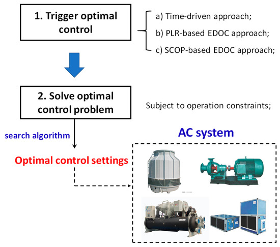
Figure 1.
Overview of the research.
A case commercial AC system is simulated in the Transient System Simulation Tool (TRNSYS) with validated component models. The optimal control codes and basic local control codes are programmed in MATLAB. Actual weather and cooling load data are used as the simulation inputs. The actual system operation is simulated through co-simulation between TRNSYS and MATLAB (Figure 2). Typical weather and load profiles are tested with each case in 24 h. The typical load profiles are identified using a PPA-based K-means clustering approach (see Appendix D). At last, the simulation results are compared to evaluate the performance.
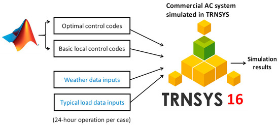
Figure 2.
Simulation diagram and software.
2.2. Optimal Control Triggering Approaches
2.2.1. PLR-based EDOC Approach
For PLR-based EDOC, “PLR significant change” and “chiller operating number change” are used as the events. The PLR is a continuous variable, and a threshold is critical for the event definition [11]. Till now, there is no selection or calculation method on this PLR variation threshold. The American Society of Heating, Refrigerating and Air-Conditioning Engineers (ASHRAE) handbook’s heating, ventilation, and air conditioning (HVAC) applications (in Section 3.2 of Chapter 42) suggests an example of 10% for the threshold of chilled-water load change. For a certain system, [10] suggested that the threshold of PLR variation can be customized for a better energy performance. This study will choose a suitable threshold from 5% to 10%.
2.2.2. SCOP-based EDOC Approach
The basic idea of the SCOP-based EDOC is to control the deviation between the current SCOP and its ideal SCOP within an acceptable range. The SCOP is defined by
where Qsys,tot is the system total cooling capacity (kW), and Psys,tot is the system total power of all the major equipment (kW).
Two events are defined to capture the transient and cumulative SCOP deviations.
Event 1: The transient SCOP deviation (which deviates from its desired value) is larger than .
where is a time index; is the reference of SCOP; and is a predefined threshold.
Event 1 actually defines an unacceptable SCOP curve, denoted by the curve in Figure 3, the value of which is calculated by . Event 1 occurs at every moment when the SCOP curve crosses the curve downward, which indicates the SCOP becoming unacceptable, and thus the optimization should be taken immediately to improve the SCOP.
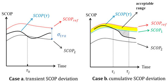
Figure 3.
Two events of SCOP deviations.
It is possible that the SCOP is lower than a certain value in a long period, but does not cross down the unacceptable curve (). In this situation, if no optimal control is taken, the operation efficiency cannot be guaranteed in the long run. Therefore, an event dedicated for the cumulative SCOP deviation is defined as below:
Event 2: The cumulative SCOP deviation is larger than .
where and are start and end time of a continuous period; is a bound to define the acceptable SCOP range; and is a predefined threshold.
Note that in Event 2, to exclude the model uncertainty in the calculation of the cumulative SCOP deviation, is used instead of in the integration. The curves and , as shown in Figure 3b, define a range in which the SCOP is acceptable. The calculation of the cumulative deviation should start only when the SCOP goes into the range . The calculation will stop, and the cumulative deviation value will be reset to zero when Event 2 or Event 1 occurs.
In the event detection, the SCOP deviation is calculated based on the measured data that are collected at each sampling time [10]. Considering the discrete-time sampling, “SCOP·mins” is used to approximate the integration in Equation (3). One minute is used as the discretization time interval to approximate the integration, as one minute is small enough for sampling time intervals in buildings. The cumulative SCOP deviation is represented by in Equation (4), where the integration is approximated by a summation.
2.3. Ideal SCOP Model
To develop the Artificial Neural Network (ANN)-based SCOP ideal (SCOPidl) model, important variables affecting the SCOP should firstly be identified. A crucial step is to select the input variables, since the inclusion of unimportant variables may bring in redundant information and decrease the ANN model accuracy [25].
Traditional techniques, e.g., correlation coefficient, standard regression coefficient and the products of these two coefficients, are inadequate to handle correlated data [26]. Thus, advanced techniques are required, such as variance-decomposition-based, variable-transformation-based and machine-learning-based techniques [26,27]. The random forest (RF) algorithm is selected because RF can handle highly correlated variables, avoid overfitting and improve the prediction accuracy. Moreover, the variable importance can be represented by “%IncMSE” from RF [28]. The calculation details of “%IncMSE” are shown in Appendix A.
To develop the prediction model of SCOPidl, the ANN algorithm is used since ANN has demonstrated its capability in handling complex relationships in building energy fields [29,30]. A typical three-layer feed-forward ANN (including the input layer, the hidden layer and the output layer) is used in this study (see Figure 4). The identified important variables are used as the ANN model inputs, while the SCOPidl is the ANN output. The ANN toolbox in MATLAB is used, and the Levenberg–Marquardt algorithm (see “trainlm” of MATLAB) is adopted in the training. A different number of hidden neurons are tested to select a suitable number, where the mean squared error (MSE) is used for the model evaluation.
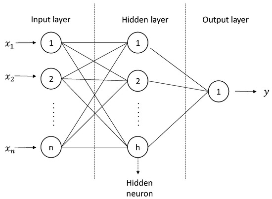
Figure 4.
The structure of the Artificial Neural Network (ANN).
3. Case Study: System, Problem Formulation and Simulation
The selected case air-conditioning system serves a super-tall office building in Hong Kong. As Hong Kong is a subtropical region, only cooling is considered in the case study.
3.1. System Description
The schematic diagram is shown in Figure 5, which is a typical primary-constant and secondary-variable chilled water system. The specifications of its main components are presented in Table 1. Four critical temperatures are controlled by PI controllers, namely the supply cooling water temperature (), the supply chilled water temperature at the primary () and secondary loops (), and the supply air temperature (). is controlled through varying the cooling tower fan frequency; is controlled by modulating the refrigerant flow rate; is controlled by modulating the water flow rate; is controlled by AHUs. The set-points of the above four critical temperatures are optimized and reset in real-time to achieve the best energy efficiency.
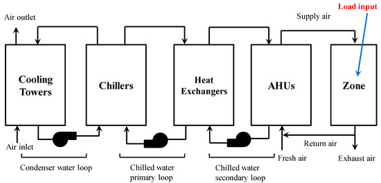
Figure 5.
Schematic of the air-conditioning (AC) system.

Table 1.
Specifications of the main components.
3.2. Optimal Control Problem Formulation
For all-electric AC systems without thermal storage, the minimization of the energy use can be simplified as the minimization of the system total power at each time instance [16]. In this case study, the decision variables that significantly affect the energy efficiency of the system operation are , , and . Thus, the real-time optimal control problem is formulated as
where .
The system total power can be written as a function of these four decision variables
where is always a nonlinear function. The decision variables are limited in their feasible ranges, which are treated as operational constraints (shown in Equations (7)–(10)).
Table 2.
Operational constraints of the case AC system [11].
3.3. Simulation Platform
A dynamic simulation platform integrating TRNSYS and MATLAB was constructed to test the performance of the proposed optimal control approaches. The platform layout was shown in Figure 6. The used TRNSYS models were verified by measured data with acceptable model accuracies. The model details are presented in Table 3. The control logics presented in Section 2 were coded in MATLAB. The simulation duration for each run was 24 h, with a simulation time step of 30 s. Several typical loads and weather data are simulated. The computer used to perform the simulation has a six-core processor (3.60 GHz) with 16 GB RAM. Since cooling load and weather data are crucial for the AC optimal control, actual load and weather data were input to the TRNSYS simulation to mimic the actual operations. The airflow rate was calculated based on the cooling load and the enthalpy difference between the supply air (the temperature set-point with 95% relative humidity) and the room air (set as 25 °C with 50% relative humidity).
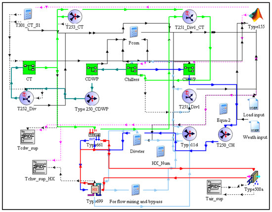
Figure 6.
Transient System Simulation Tool (TRNSYS) model (screenshot).
Table 3.
TRNSYS model and description.
3.4. Ideal SCOP Model
To develop an ANN model for predicting the ideal SCOP, important variables that have significant influence on the SCOP were firstly identified. Basically, important variables that affect the SCOP are similar in typical AC systems that contain chillers, cooling towers, pumps and AHUs/Coils [16,32]. The variables include the outdoor dry/wet-bulb temperature (/), the chilled water supply temperature (), the condensing water return temperature (), the chilled water mass flow rate at the primary/secondary loop (/), the PLR, the cooling tower fan frequency () and the enthalpy driving force in the operation of cooling towers “” [33].
To evaluate the variable importance, the RF algorithm was implemented in the software R using the package of “randomForest” [34] and the results were plotted in Figure 7. The variable PLR has the highest importance, while the has the lowest importance. As discussed in [35], less important variables (e.g., % IncMSE lower than 10%) can be omitted. Therefore, was not used in the ideal SCOP model, and totally eight variables were used as the ANN model inputs.
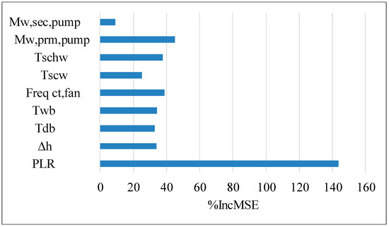
Figure 7.
Results of random forest (higher %IncMSE means more important).
In the ANN model, 70% of the data set was used for training, 15% of the data set was used for validation and the additional 15% of the data set was used to test whether the model can perform well. Since the optimal number of the hidden layer neurons depends upon the specific problem, this study tested a different number of hidden neurons (from 2 to 20). The MSEs of different numbers of hidden neurons were plotted in Figure 8. Figure 8. shows that when the number of neurons increased, the MSE decreased. However, the reduction in MSE became insignificant as the number of neurons was greater than 15. Thus, “15” was selected as the optimal number of hidden neurons. The R-value of the ANN model with 15 hidden neurons was 0.96052 (see Figure 9), with R values of training, validation and test are 0.96007, 0,95783 and 0.9656 respectively, which showed a good prediction accuracy.
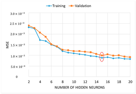
Figure 8.
Number of ANN hidden neurons vs. mean squared error (MSE).
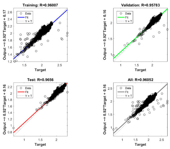
Figure 9.
Regression plots of the ANN model (with “15” hidden neurons).
3.5. Event Threshold
For the event “PLR significant change”, 7% was selected as the PLR change threshold based on a previous study on the same AC system [11]. The threshold of SCOP deviation can be calculated based on the value of SCOPidl and an expected energy saving percentage (as shown in Appendix C Equation (A8)). For instance, an expected energy saving percentage can be specified by users (e.g., 10%), and the SCOPidl can be obtained from the developed ANN model. After the threshold is calculated, it should be checked that whether the calculated threshold is feasible or not based on the SCOP deviations in historical data. The threshold selection should also consider the uncertainties in the SCOPidl model and SCOP measurement in terms of the application concerns.
The thresholds of the SCOP deviation are set as 0.2057 (transient) and 2.057 (cumulative). The selection details are presented as follows: The targeted energy saving is set as 10%, based on handbook [16] and a previous study [10]. To help the threshold selection, the histogram of SCOPidl and SCOP deviation are plotted in Figure 10. The base case keeps all the four temperature set-points as constant. The SCOP deviation is the difference between SCOP of the base case and SCOPidl. From Figure 10, the mean of SCOPidl is 2.0544. Using a SCOPidl of 2.0544 and an expected energy saving of 10.0%, the threshold of SCOP deviation is 0.2057, based on Equation (A8) (Appendix C).
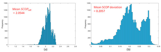
Figure 10.
(a) Histogram of SCOPidl; (b) Histogram of SCOP deviation.
Since “0.2057” is within the range of SCOP deviation and the most frequent case (Figure 10b), it is a feasible threshold value.
For uncertainties, the value 0.01 was used for as the model uncertainty of SCOPidl, which was the averaged value over the training and validation Mean Squared Error (MSE) of the ANN model. The measurement uncertainty for the case study was calculated in Appendix B, where sensor uncertainties were added to the simulation-generated operation data. As a negative value is considered, “–0.0694” was used for measurement uncertainty. Thus, the combined uncertainty is “–0.0794” (“–0.01”+”–0.0694”), and can be set as “”.
In comparison, the threshold 0.2057 is nearly three times greater the combined uncertainty, which can largely prevent the uncertainty-caused event triggering. Thus, 0.2057 is used as the threshold of transient SCOP deviation. The cumulative SCOP deviation depends on both the time duration and the SCOP deviation. The deviation for cumulative SCOP was considered as half of the transient SCOP deviation threshold (i.e., 0.2057/2), or a 5% energy saving equivalently. The time duration was selected as 20 minutes for a demonstration. Thus, the threshold of cumulative SCOP deviation is 2.057.
4. Results and Discussions
4.1. Energy Performance
The optimal control performance is evaluated by the energy saving percentage. The energy saving percentage is computed based on the base case (i.e., constant control settings without optimal control). The energy saving percentages of EDOC range from 5.83% to 12.06% for ten different load clusters. In general, as can be seen from Figure 11, SCOP-based EDOC outperforms PLR-based EDOC, and EDOC outperforms TDOC (1 h per optimal control).
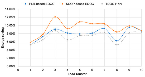
Figure 11.
Energy saving percentages.
The biggest energy performance difference can be 3%, as shown in load cluster no. 3. The possible reason of such superior performance is that the SCOP-based events can directly represent the system operation efficiency without mismatch compared with the PLR-based events. By continuous monitoring and tracking of the transient and cumulative SCOP deviations, a better timing of optimal control can be achieved. As a result, the system operation efficiency is always maintained at or near the ideal level. The next section will discuss the triggering time of optimal control in details.
4.2. Triggering Time of Optimal Control
It was observed that (see Table 4), in load cluster 1, both TDOC and EDOC approaches triggered seven times control actions. Thus, load cluster 1 is the best for analyzing the effect of different optimal control triggering times.
Table 4.
Optimal control triggering frequency of EDOC.
In Figure 12, the optimal control time of EDOC is plotted. The Y axis refers to the time of the optimal control action, and the Y axis is updated each time when this optimal control is triggered. The X axis is the simulation time step in minutes. From Figure 12 (see dashed circles), SCOP-based EDOC tends to react in advance compared to the PLR-based EDOC. The possible reason is because SCOP is a more comprehensive energy efficiency index than the PLR index. SCOP-based EDOC can capture the operation variation earlier than the PLR-based EDOC, leading to a better energy performance. Moreover, inside the solid circles of Figure 12, the SCOP-based EDOC did not take response, while this PLR-based EDOC triggered optimal control. In such circumstances, the PLR varies, but the SCOP still remains at the ideal level, which is unnecessary to trigger optimal control. The SCOP-based EDOC could avoid such unnecessary actions, while the PLR-based EDOC cannot (which is a demerit).
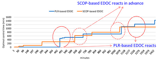
Figure 12.
Optimal control time of EDOC (load cluster 1).
The total optimal control times of EDOC are shown in Table 4, which reflects the frequency of optimal control. Based on literatures [15,36,37], it can be found that 1 h per optimal control is the most common optimal control frequency used for TDOC. Thus, this study uses 1 h as the benchmark. Then, less than 24 times can be regarded as an acceptable triggering frequency for one day. On average, PLR-based EDOC (22.7 times per day) satisfies the condition, while SCOP-based EDOC (26.4 times per day) triggers more actions than the benchmark. It should be noted that, in load cluster no. 8, the SCOP-based EDOC performed 61 times of optimal control. The reason for such frequent triggering is possibly due to the uncertainty in “SCOP”. As the parameter, SCOP is calculated based on the power meter and the load measurement, the combined uncertainty of power and load could be significant. Besides, the model of ideal SCOP also has model uncertainty. When the SCOP value fluctuated at the pre-defined threshold value, the optimal control action can be triggered frequently. From this, a demerit of SCOP-based EDOC is that frequent optimal control may be triggered compared with PLR-based EDOC. This problem could be mitigated by adding an additional time interval constraint between two adjacent optimal control actions (e.g., at least 10 mins between two control actions). Although SCOP-based EDOC obtains the highest energy saving, in terms of the energy saving performance, triggering frequency and robustness of optimal control, PLR-based EDOC can still be recommended to replace traditional TDOC for practical applications.
4.3. Analyses of SCOP-based Events
As both transient and cumulative SCOP deviations are used (Section 2.2.2), the event triggering times of the two events are analyzed in this section. From Figure 13, and were triggered differently under different load clusters, sometimes dominates, and sometimes reacts more. For example, in load cluster C1 and C2, only was triggered. In load cluster C3–C10, and both appeared. If only using in load cluster C1 and C2, the SCOP-based EDOC may not work. This validates the idea of combing and to accommodate broader operation conditions, since one event may fail sometimes.
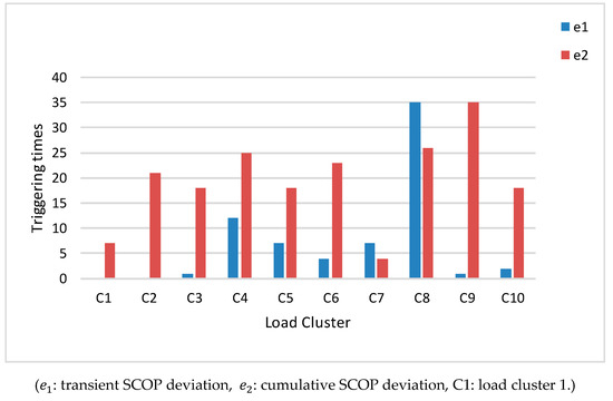
Figure 13.
Triggering times of SCOP-based events.
Regarding the individual energy performance of the single event (and ), load cluster C7 was used as an illustration, where two events are triggered almost equally. Simulation results show: Using only gives 9.84% of energy saving, and using only gives 9.97% of energy saving. In Figure 11, combining and outputs 10.38% of energy saving. It can be seen that combining and will be beneficial for improving the energy performance of EDOC. The reason is because the single event may not capture the critical operation variations in a comprehensive manner.
5. Conclusions
This study investigates the optimal control triggering of EDOC in AC systems. Optimal control triggering approaches are classified into direct and indirect approaches based on the used triggering indicator. In the direct SCOP-based EDOC, two events have been defined to capture both the transient and cumulative SCOP deviations, which maintains the SCOP at the ideal level in a closed-loop manner. Simulated case studies suggest that direct SCOP-based EDOC achieved a higher energy saving than indirect PLR-based EDOC in all the typical load scenarios. The main reason is due to a more direct performance indicator, i.e., SCOP, that can reflect the system performance precisely and timely. However, the development of an accurate ideal SCOP model requires sufficient operation data and extensive work, which could restrict its implementation [8]. The robustness issues caused by the uncertainty of SCOP should also be paid attention to. Thus, in terms of actual applications, the SCOP-based EDOC can be recommended when the ideal SCOP model is available with a properly-handled uncertainty issue. However, the PLR-based EDOC could still be a more practical option to replace traditional TDOC, which features an easy development process, better robustness and acceptable energy performance.
Author Contributions
Conceptualization, J.W.; Data curation, R.L. and L.Z.; Formal analysis, H.S.A. and E.M.; Funding acquisition, J.W.; Investigation, R.L.; Methodology, J.W.; Resources, L.Z.; Supervision, J.W.; Validation, H.S.A. and E.M.
Funding
This research was funded by Natural Science Foundation of Jiangsu Province (BK20190942), Suzhou University of Science and Technology Research projects funding for the introducing talents (331911204), Comprehensive curriculum reform program (2018KJZG-09), and Suzhou science and technology plan projects (SNG2017052).
Acknowledgments
The authors would acknowledge to the Staffs of City University of Hong Kong for their supports.
Conflicts of Interest
The authors declare no conflict of interest.
Nomenclature
| Variables/Abbreviations | Subscripts | ||
| SCOP | system coefficient of performance | scw | supply cooling water |
| EDOC | event-driven optimal control | schw | supply chilled water |
| TDOC | time-driven optimal control | sa | supply air |
| TLP | typical load profile | prm | primary |
| PLR | part-load ratio | sec | secondary |
| SCOP | system coefficient of performance | wb | wet-bulb |
| s | event threshold | db | dry-bulb |
| T | Temperature (°C) | sys | system |
| P | Power (kW) | tot | total |
| Mw | water flow rate (L/s) | ct | cooling tower |
| Freq | Frequency (Hz) | ch | chiller |
| PAA | Piecewise Aggregate Approximation | pump | pump |
| enthalpy difference between the saturated (at cooling tower inlet water temperature) and incoming air of cooling tower (kJ/kg) | fan | fan | |
| ref | reference value | ||
| lower | lower bound | ||
| upper | upper bound | ||
Appendix A. Variable Importance Measures (“%IncMSE”)
In the random forest algorithm, the variable importance is represented by “%IncMSE”.
where “” stands for the MSE if is not used in the prediction. A higher suggests that the variable is more important.
Appendix B. SCOP Measurement Uncertainty
This part is to calculate the measurement uncertainty of SCOP. The equations for SCOP are shown in (A2)–(A4), where is the system cooling capacity, and are the water specific heat capacity and water flow rate (others please see the nomenclature). Assuming the sensors/meters are well-calibrated, the reported accuracies of sensors/meters from a chiller design guide [38] can be used to quantify the measurement uncertainty of SCOP.
Considering the measurement uncertainties in the cooling capacity and power, the Equation (A2) can be re-written as Equation (A5), where the subscript means the measured value, , and are the measurement uncertainties for the power, cooling capacity and SCOP.
where
Since multiple uncertainties are involved in the SCOP calculation, uncertainty shift can be used to integrate the variable uncertainties for easy analyses [39]. The measurement uncertainty of power consumption can be easily quantified by the power meter uncertainty. For the measurement uncertainty of the cooling capacity, the measured cooling capacity is represented by Equation (A6), and the measurement uncertainty can be calculated by Equation (A7), as demonstrated by [39].
With where , , are the measurement uncertainties for the corresponding variables.
Based on measurement accuracies in Table A1, the measurement uncertainties of cooling capacity and power can be calculated. The simulated operation data is considered as the measured value. As presented in Table A2, the maximum positive and negative relative uncertainties for are +3.73% and -3.95%, with the absolute uncertainties of “0.0708” and “-0.0694” respectively.
Table A1.
Typical measurement accuracy [38].
Table A1.
Typical measurement accuracy [38].
| Measured Variable | Reported Accuracy |
|---|---|
| Water flow | |
| Water temperature | |
| Electrical power |
Table A2.
Measurement uncertainties of SCOP (worst cases).
Table A2.
Measurement uncertainties of SCOP (worst cases).
| Relative SCOP Measurement Uncertainty | Absolute SCOP Measurement Uncertainty | ||||
|---|---|---|---|---|---|
| +1% of full scale | +0.2°C | 197 kW | −38.01 kW (−1% of reading) | +3.73% | +0.0708 |
| −1% of full scale | −0.2°C | −197 kW | +38.01 kW (+1% of reading) | −3.95% | −0.0694 |
Appendix C. Energy Saving Estimation
The energy saving percentage at a time instant can be estimated using Equation (A8) by substituting the value of and .
where P is power, idl is the ideal value, is the time instant.
Appendix D. Load Clustering
A K-means clustering method is proposed to generate typical load profiles (TLPs) in this study. Figure A1a shows a general procedure of the K-means clustering with a Piecewise Aggregate Approximation (PAA) transformation. To cluster the load profile (a time-series data), the distance between two profiles should be computed for measuring the similarity. However, computing the distance on raw time-series data is difficult and slow. Therefore, the approximation is normally carried out to reduce the computational difficulties [40]. Many representation techniques can be used to transform the raw time-series data, such as Discrete Fourier Transformation [41], Discrete Wavelet Transformation [42], Single Value Decomposition [43], PAA [44], etc. The PAA was used in this paper due to its simplicity and fast calculation speed [44].
In the PAA method, the original load profile is firstly segmented into equal-distance pieces (Figure A1b). Then, the mean of each piece is used to approximate the original segment (Figure A1c). This approximation greatly reduces the data dimension, while the fundamental characteristics in the original time-series data are still captured. After the PAA transformation, the Euclidean distance between two load profiles is calculated, and the standard K-means clustering algorithm is applied. The initialization of the K-means is important as it affects the final result [45]. A different K value will be tested to find a suitable one. A realistic testing range for the K value is between 2 and √n [46], where “n” is the number of data samples. Then, the “furthest first initialization” is used, which starts at a random point as the first cluster center, and adding more cluster centers which are furthest from the existing ones [47]. Based on the clustering result, one representative profile from each cluster will be selected to form the TLPs.
The measured cooling load data of the case building in year 2013 was used. In total 214 daily load profiles from spring season to autumn season were used, which covered typical cooling seasons for sub-tropical regions like Hong Kong. The clustered loads were given in Figure A2a, where the similar load profiles were grouped together as a load cluster. In each cluster, the load profile closest to the cluster centroid was selected to constitute the TLPs (see Figure A2b). These TLPs and their associated weather data (from Hong Kong Observatory) were used as the simulation inputs.

Figure A1.
(a) Process of generating typical load profiles (TLPs); (b) two original load profiles; (c) two load profiles after PAA transformation.

Figure A2.
(a) Clustered load profiles; (b) Selected typical load profiles.
Table A3.
Load and weather data of ten TLPs.
Table A3.
Load and weather data of ten TLPs.
| Load Cluster. | Load (kW) | Tdb (°C) | Twb (°C) | ||||||
|---|---|---|---|---|---|---|---|---|---|
| Mean | Max | Min | Mean | Max | Min | Mean | Max | Min | |
| C1# | 4833 | 6495 | 3268 | 21.5 | 23.5 | 20.6 | 18.8 | 19.7 | 17.4 |
| C2 | 9072 | 13038 | 3954 | 23.7 | 25.2 | 22.1 | 22.9 | 23.6 | 21.5 |
| C3 | 13998 | 22361 | 4212 | 29.7 | 32.9 | 27.6 | 26.6 | 28.1 | 25.9 |
| C4 | 6164 | 8593 | 3437 | 29.2 | 32.5 | 27.3 | 26.2 | 27.4 | 25.3 |
| C5 | 14492 | 22996 | 2923 | 29.7 | 33.1 | 27.4 | 26.1 | 27.9 | 24.9 |
| C6 | 12646 | 21177 | 3367 | 28.2 | 31.0 | 26.4 | 25.3 | 26.0 | 24.4 |
| C7 | 11465 | 17715 | 3740 | 27.8 | 29.7 | 26.8 | 24.0 | 25.1 | 22.8 |
| C8 | 7037 | 10241 | 3355 | 29.2 | 31.9 | 27.2 | 26.1 | 27.1 | 25.1 |
| C9 | 8067 | 18175 | 3475 | 31.2 | 34.2 | 28.4 | 25.1 | 26.8 | 23.5 |
| C10 | 10628 | 15714 | 3487 | 24.8 | 27.3 | 22.9 | 21.5 | 22.5 | 19.5 |
(#: ‘C1′ means the load cluster 1.).
References
- Ahmad, M.W.; Mourshed, M.; Yuce, B.; Rezgui, Y. Computational intelligence techniques for HVAC systems: A review. Build. Simul. 2016, 9, 359–398. [Google Scholar] [CrossRef]
- Liu, Z.; Song, F.; Jiang, Z.; Chen, X.; Guan, X. Optimization based integrated control of building HVAC system. Build. Simul. 2014, 7, 375–387. [Google Scholar] [CrossRef]
- Sun, Y.; Huang, G. Recent Developments in HVAC System Control and Building Demand Management. Curr. Sustain. Renew. Energy Rep. 2017, 4, 15–21. [Google Scholar] [CrossRef]
- Kim, J.-H.; Seong, N.-C.; Choi, W. Modeling and Optimizing a Chiller System Using a Machine Learning Algorithm. Energies 2019, 12, 2860. [Google Scholar] [CrossRef]
- Zhang, S.; Cheng, Y.; Fang, Z.; Lin, Z. Dynamic Control of Room Air Temperature for Stratum Ventilation Based on Heat Removal Efficiency: Method and Experimental Validations. Build. Environ. 2018, 140, 107–118. [Google Scholar] [CrossRef]
- Zhang, S.; Cheng, Y.; Fang, Z.; Huan, C.; Lin, Z. Optimization of room air temperature in stratum-ventilated rooms for both thermal comfort and energy saving. Appl. Energy 2017, 204, 420–431. [Google Scholar] [CrossRef]
- Wang, S.; Ma, Z. Supervisory and optimal control of building HVAC systems: A review. HVAC&R Res. 2008, 14, 3–32. [Google Scholar]
- Atam, E. New Paths Toward Energy-Efficient Buildings: A Multiaspect Discussion of Advanced Model-Based Control. IEEE Ind. Electron. Mag. 2016, 10, 50–66. [Google Scholar] [CrossRef]
- Asad, H.S.; Yuen, R.K.K.; Liu, J.; Wang, J. Adaptive modeling for reliability in optimal control of complex HVAC systems. Build. Simul. 2019, 12, 1095–1106. [Google Scholar] [CrossRef]
- Wang, J.; Jia, Q.; Huang, G.; Sun, Y. Event-driven optimal control of central air-conditioning systems: Event-space establishment. Sci. Technol. Built Environ. 2018, 24, 839–849. [Google Scholar] [CrossRef]
- Wang, J.; Huang, G.; Sun, Y.; Liu, X. Event-driven optimization of complex HVAC systems. Energy Build. 2016, 133, 79–87. [Google Scholar] [CrossRef]
- Wang, J.; Huang, G.; Zhou, P. Event-driven optimal control of complex HVAC systems based on COP mins. Energy Procedia 2017, 105, 2372–2377. [Google Scholar] [CrossRef]
- Darby, M.L.; Nikolaou, M.; Jones, J.; Nicholson, D. RTO: An overview and assessment of current practice. J. Process Control 2011, 21, 874–884. [Google Scholar] [CrossRef]
- Kusiak, A.; Li, M.; Tang, F. Modeling and optimization of HVAC energy consumption. Appl. Energy 2010, 87, 3092–3102. [Google Scholar] [CrossRef]
- Huang, S.; Zuo, W.; Sohn, M.D. Improved cooling tower control of legacy chiller plants by optimizing the condenser water set point. Build. Environ. 2017, 111, 33–46. [Google Scholar] [CrossRef]
- ASHRAE 2015. Chapter 42–Supervisory control strategies and optimization. In ASHRAE Handbook–HVAC Applications; ASHRAE Inc.: New York, NY, USA, 2011. [Google Scholar]
- Saeedi, M.; Moradi, M.; Hosseini, M.; Emamifar, A.; Ghadimi, N. Robust optimization based optimal chiller loading under cooling demand uncertainty. Appl. Therm. Eng. 2019, 148, 1081–1091. [Google Scholar] [CrossRef]
- Braun, M.R.; Walton, P.; Beck, S.B.M. Illustrating the relationship between the coefficient of performance and the coefficient of system performance by means of an R404 supermarket refrigeration system. Int. J. Refrig. 2016, 70, 225–234. [Google Scholar] [CrossRef]
- Huang, S.; Zuo, W.; Sohn, M.D. Amelioration of the cooling load based chiller sequencing control. Appl. Energy 2016, 168, 204–215. [Google Scholar] [CrossRef]
- Yan, C.; Gang, W.; Niu, X.; Peng, X.; Wang, S. Quantitative evaluation of the impact of building load characteristics on energy performance of district cooling systems. Appl. Energy 2017, 205, 635–643. [Google Scholar] [CrossRef]
- Yu, F.W.; Chan, K.T. Economic benefits of optimal control for water-cooled chiller systems serving hotels in a subtropical climate. Energy Build. 2010, 42, 203–209. [Google Scholar] [CrossRef]
- Xu, Z.; Hu, G.; Spanos, C.J.; Schiavon, S. PMV-based event-triggered mechanism for building energy management under uncertainties. Energy Build. 2017, 152, 73–85. [Google Scholar] [CrossRef]
- Du, Z.; Jin, X.; Fang, X.; Fan, B. A dual-benchmark based energy analysis method to evaluate control strategies for building HVAC systems. Appl. Energy 2016, 183, 700–714. [Google Scholar] [CrossRef]
- Fang, X.; Jin, X.; Du, Z.; Wang, Y. The evaluation of operation performance of HVAC system based on the ideal operation level of system. Energy Build. 2016, 110, 330–344. [Google Scholar] [CrossRef]
- Ding, Y.; Zhang, Q.; Yuan, T.; Yang, F. Effect of input variables on cooling load prediction accuracy of an office building. Appl. Therm. Eng. 2018, 128, 225–234. [Google Scholar] [CrossRef]
- Bi, J. A review of statistical methods for determination of relative importance of correlated predictors and identification of drivers of consumer liking. J. Sens. Stud. 2012, 27, 87–101. [Google Scholar] [CrossRef]
- Tian, W. A review of sensitivity analysis methods in building energy analysis. Renew. Sustain. Energy Rev. 2013, 20, 411–419. [Google Scholar] [CrossRef]
- Archer, K.J.; Kimes, R.V. Empirical characterization of random forest variable importance measures. Comput. Stat. Data Anal. 2008, 52, 2249–2260. [Google Scholar] [CrossRef]
- Wang, Z.; Srinivasan, R.S. A review of artificial intelligence based building energy use prediction: Contrasting the capabilities of single and ensemble prediction models. Renew. Sustain. Energy Rev. 2017, 75, 796–808. [Google Scholar] [CrossRef]
- Zhao, L.; Liu, Z.; Mbachu, J. Energy Management through Cost Forecasting for Residential Buildings in New Zealand. Energies 2019, 12, 2888. [Google Scholar] [CrossRef]
- Ma, Z. Online Supervisory and Optimal Control of Complex Building Central Chilling Systems. Ph.D. Thesis, The Hong Kong Polytechnic University, Hong Kong, China, 2008. [Google Scholar]
- Yoon, Y.R.; Moon, H.J. Energy Consumption Model with Energy Use Factors of Tenants in Commercial Buildings Using Gaussian Process Regression. Energy Build. 2018, 168, 215–224. [Google Scholar] [CrossRef]
- Chang, C.; Shieh, S.; Jang, S.; Wu, C.; Tsou, Y. Energy conservation improvement and ON–OFF switch times reduction for an existing VFD-fan-based cooling tower. Appl. Energy 2015, 154, 491–499. [Google Scholar] [CrossRef]
- Breiman, L.; Cutler, A.; Liaw, A.; Wiener, M. Breiman and Cutler’s Random Forests for Classification and Regression; 2015; The R Project for Statistical Computing; Available online: https://www.researchgate.net/publication/304378707_Package_‘randomForest’_Breiman_and_Cutler’s_random_forests_for_classification_and_regression (accessed on 9 September 2019).
- Yu, F.; Ho, W.; Chan, K.; Sit, R. Critique of operating variables importance on chiller energy performance using random forest. Energy Build. 2017, 139, 653–664. [Google Scholar] [CrossRef]
- Wei, X.; Kusiak, A.; Li, M.; Tang, F.; Zeng, Y. Multi-objective optimization of the HVAC (heating, ventilation, and air conditioning) system performance. Energy 2015, 83, 294–306. [Google Scholar] [CrossRef]
- Mossolly, M.; Ghali, K.N.; Ghaddar, N. Optimal control strategy for a multi-zone air conditioning system using a genetic algorithm. Energy 2009, 34, 58–66. [Google Scholar] [CrossRef]
- EDR. Chilled Water Plant Design Guide; EDR, 2009; Available online: https://www.google.com.hk/url?sa=t&rct=j&q=&esrc=s&source=web&cd=1&ved=2ahUKEwj19YKenJblAhVBMN4KHVqDATQQFjAAegQIAhAC&url=http%3A%2F%2Fwww.taylor-engineering.com%2FWebsites%2Ftaylorengineering%2Fimages%2Fguides%2FEDR_DesignGuidelines_CoolToolsChilledWater.pdf&usg=AOvVaw3bjt6a4g9we8XKcaXHHeN (accessed on 9 September 2019).
- Liao, Y.; Huang, G.; Sun, Y.; Zhang, L. Uncertainty analysis for chiller sequencing control. Energy Build. 2014, 85, 187–198. [Google Scholar] [CrossRef]
- Yildiz, B.; Bilbao, J.; Dore, J.; Sproul, A. Recent advances in the analysis of residential electricity consumption and applications of smart meter data. Appl. Energy 2017, 208, 402–427. [Google Scholar] [CrossRef]
- Li, X.; Li, F.; Chen, S.; Li, Y.; Zou, Q.; Wu, Z.; Lin, S. An Improved Commutation Prediction Algorithm to Mitigate Commutation Failure in High Voltage Direct Current. Energies 2017, 10, 1481. [Google Scholar] [CrossRef]
- Li, S.; Wen, J. A model-based fault detection and diagnostic methodology based on PCA method and wavelet transform. Energy Build. 2014, 68, 63–71. [Google Scholar] [CrossRef]
- Lü, X.; Lu, T.; Kibert, C.J.; Viljanen, M. A novel dynamic modeling approach for predicting building energy performance. Appl. Energy 2014, 114, 91–103. [Google Scholar] [CrossRef]
- Keogh, E.; Chakrabarti, K.; Pazzani, M.; Mehrotra, S. Dimensionality reduction for fast similarity search in large time series databases. Knowl. Inf. Syst. 2001, 3, 263–286. [Google Scholar] [CrossRef]
- Steinley, D.; Brusco, M.J. Initializing k-means batch clustering: A critical evaluation of several techniques. J. Classif. 2007, 24, 99–121. [Google Scholar] [CrossRef]
- Ren, X.; Yan, D.; Hong, T. Data mining of space heating system performance in affordable housing. Build. Environ. 2015, 89, 1–13. [Google Scholar] [CrossRef]
- Jin, X.; Han, J. K-means clustering. In Encyclopedia of Machine Learning; Springer: Berlin, Germany, 2011; pp. 563–564. [Google Scholar]
© 2019 by the authors. Licensee MDPI, Basel, Switzerland. This article is an open access article distributed under the terms and conditions of the Creative Commons Attribution (CC BY) license (http://creativecommons.org/licenses/by/4.0/).