Operation Optimization of Multi-District Integrated Energy System Considering Flexible Demand Response of Electric and Thermal Loads

Abstract

Multi-district integrated energy system (IES) can make full use of the complementary characteristics of district power and thermal system, and loads in different districts. It can improve the flexibility and economy of system operation, which has a good development prospect. Firstly, based on the general energy transfer model of the district heating network (DHN), the DHN system is described by the basic equations of the heating network and nodes considering the characteristics of the transmission time delay and heat loss in pipelines. A coupling model of DHN and multi-district IES is established. Secondly, the flexible demand response (FDR) model of electric and thermal loads is established. The load characteristics of each district in IES are studied. A shiftable load model based on the electric quantity balance is constructed. Considering the flexibility of the heat demand, a thermal load adjustment model based on the comfort constraint is constructed to make the thermal load elastic and controllable in time and space. Finally, a mixed integer linear programming (MILP) model for operation optimization of multi-district IES with the DHN considering the FDR of electric and thermal loads is established based on the supply and demand sides. The result shows that the proposed model makes full use of the complementary characteristics of electric and thermal loads in different districts. It realizes the coordinated distribution of thermal energy among different districts and improves the efficiency of thermal energy utilization through the DHN. FDR effectively reduces the peak-valley difference of loads. It further reduces the total operating cost by the coordinated operation of the DHN and multi-district IES.

1. Introduction

With the increasing energy demand in the industrial production and households, the contradiction has intensified between environmental problems and the energy development. Improving the energy efficiency, reducing environmental pollution, and achieving the sustainable energy development have become a major concern of academic and industrial circles in recent years [1,2,3]. Energy Internet [4] and integrated energy system (IES) [5] have been put forward and studied by scholars worldwide. It establishes a vision of the broad interconnection and equal sharing of energy systems in the future and provides new ideas for efficient and economic utilization of energy. At present, the planning and operation of IES is usually based on the combined cooling, heating, and power (CCHP) system in a single area. The equipment selection and operation management are carried out to achieve the district optimization according to load characteristics in one area [6,7]. However, the load characteristics in a specific area are often relatively monotonic, which will affect the optimization result to a certain extent [8,9]. Multi-district IES can couple the cooling and thermal loads of each area through the interconnection of the cooling and heating network. Due to the obvious interlacing phenomenon of peak and valley in each district, the complementarity of loads can be fully utilized, and the thermal output of each CCHP system can be coordinated to match the cooling and thermal demand. Finally, the optimal dispatch of energy will be realized to further improve the coordinated operation and operation economy of equipment in the system [10,11,12].

Establishing the interconnection model of multi-district IES and heating networks, and the operation optimization model of multi-district IES is the core of the research. In order to realize the coordinated optimization and dispatching of multi-district IES, an energy transfer model for heating networks is established, which improves the economic benefit of the IES [10]. To minimize the annual total cost and CO₂ emission, a mathematical model for the selection, configuration, operation of distributed energy system, and the collaborative optimization of the district heating network (DHN) was established [13]. Fef. [14] studies the thermoelectric joint dispatching model considering the dynamic characteristics of heating pipelines and the model of heat storage devices, which promotes the economy of the system and the wind power absorption. Fef. [7] takes a commercial and residential complex in eastern Tehran as an example. A planning model is established for seven CCHP systems interconnected by the heating network, and the optimal capacity and operation strategy of the system equipment are studied. However, the heating network model is too simplified in the paper. In order to coordinate the short-term operation of power systems with large amounts of wind power and district heating systems, a combined model of transmission-constrained unit commitment with the combined electricity and DHN is established by using the linear DHN model. The heat storage capacity of the DHN is modeled by capturing the quasi-dynamics of pipeline temperature [15].

As mentioned above, the research on IES optimal operation model is carried out from the perspective of energy supply, without considering the load characteristic on its economic optimal operation. Demand response management is an important component of the future smart grid. It contributes to reducing power peak load and variation, and economic operation [16,17]. As an important zero-emission flexible resource in the power market environment, the demand response (DR) resources can effectively improve the load demand distribution and optimize the resource allocation and tap negative energy. Mining the DR resources on the load side will further improve the operation economy and flexibility of supply and demand in multi-district IES. The DR of IES can be realized by flexible electric and thermal loads. Fef. [18,19] study the impact of flexible electric load on the economic benefits of the microgrid, and establishes an economic dispatching model of microgrid considering DR. An optimal operation framework for energy hub based on micro IES considering the multi-carrier load classification and scheduling, while the shiftable electrical load and curtailable thermal load scheduling model are added into the constraints of optimization formulation. It reduces the energy consumption cost, peak power, and heat load demand of the system [20]. Fef. [21] studies the two-dimensional controllability of the thermal load and establishes an economic dispatching model of the combined heat and power generation. Based on the traditional DR mechanism in recent literature, the DR optimization model of the coupled electric-thermal system is established considering the price and demand differences of various energy sources [22]. Fef. [23] suggests the combination of electric heating and intelligent energy storage such as water heaters, which can transfer energy consumption to the non-peak period and optimize the consumption price without affecting consumer’s comfort. However, the above-mentioned literatures seldom take into account the complementarity of electric and thermal loads, and the load characteristic in different districts.

In order to solve the above problems, a flexible demand response (FDR) model of electric and thermal loads and an operation optimization model for multi-district IES with the DHN are established from the supply and demand sides. In the coupling part of the DHN and multi-district IES, the DHN system is described by the basic equations of the heating network and nodes considering the characteristics of the transmission time delay and heat loss on heating pipelines. A coupling model of DHN and multi-district IES is established. By connecting all the districts through the DHN and utilizing the complementary characteristics of loads, the surplus energy is transferred to other districts in the form of thermal power. The heat-to-electric ratios are redistributed to improve the flexibility of the system operation. In the FDR part of electric and thermal loads, the shiftable electric load model is constructed after studying the electric load characteristics in different districts of IES. Considering the flexibility of consumer’s heating demand, a regulation model for thermal load based on the comfort constraint is constructed, which makes full use of the elasticity and adjustability of the thermal load in time and space. Finally, combining the FDR model with the coupling model of the DHN and multi-district IES, a mixed integer linear programming (MILP) model for operation optimization of multi-district IES considering the FDR of electric and thermal loads is established. The case result shows that the DHN realizes the complementary supply and demand of electricity and thermal loads, and promotes the coordinated distribution of thermal energy among different districts. FDR plays a role of shaving peak and filling valley. Based on the economic benefits brought by the operation of DHN and multi-district IES, the total operating cost is further reduced. The rationality and effectiveness of the proposed model are verified.

2. Modeling of Multi-District IES

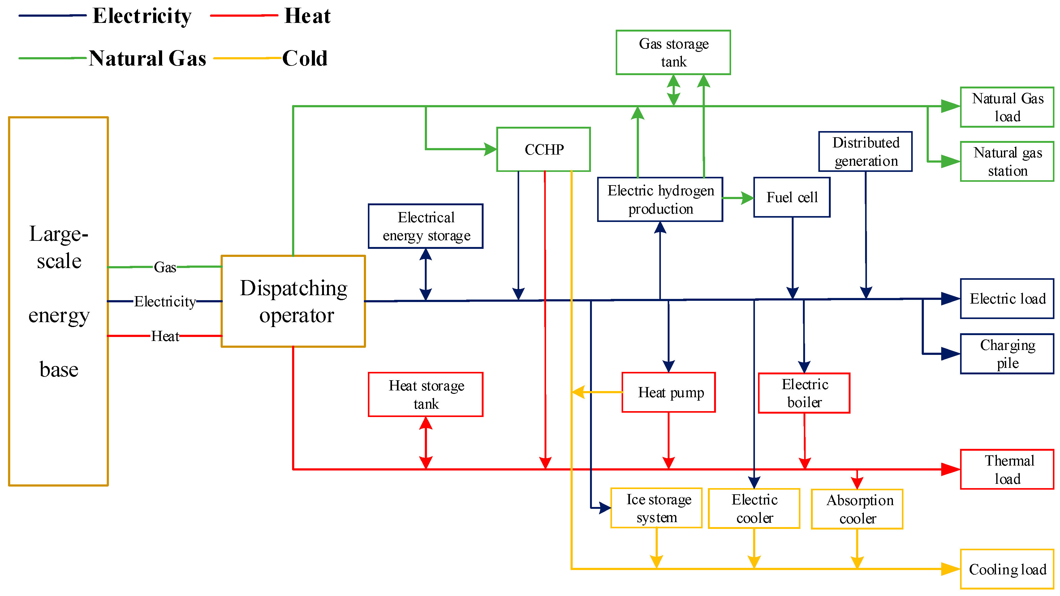
IES is a deep integration of energy and information technology. In the process of planning, construction, control and operation, the production, transmission, transformation, distribution, storage and consumption of energy are coordinated and optimized. IES is formed as the system integrating energy production, supply and marketing of cold, heat, electricity, and natural gas. Energy Internet, energy hub [24] and ubiquitous energy Internet [25] proposed in the existing research at home and abroad are all the specific manifestations of IES. They are consistent in the basic physical architecture and equipment level. According to the description of the equipment and system architecture in IES, the basic physical architecture of IES is summarized in Figure 1.

According to the energy consumption/conversion of equipment, the equipment in IES can be divided into independent equipment units and coupling equipment units. Independent equipment units consume electricity, heat, gas, and cold to maintain operation. They have no coupling transformation and complementary utilization between heterogeneous energy flows. Coupling equipment units can realize the conversion and utilization of electricity, heat, gas, and cold.

2.1. Model of Heating Networks

Heating network is a system that transfers thermal energy to thermal load through pipelines and heating medium. It is essentially a fluid network which carries thermal energy. The analysis of the heating network model is mainly to study the relationship among thermal energy, temperature and heating medium. According to different heating mediums, they can be divided into hot water networks and steam networks. In China, hot water networks are mostly used. Therefore, this paper focus on the hot water heating system as an example to establish the heating network model. This paper assumes that both the water supply temperature and the return water temperature are constant, which are 90 °C and 70 °C, respectively.

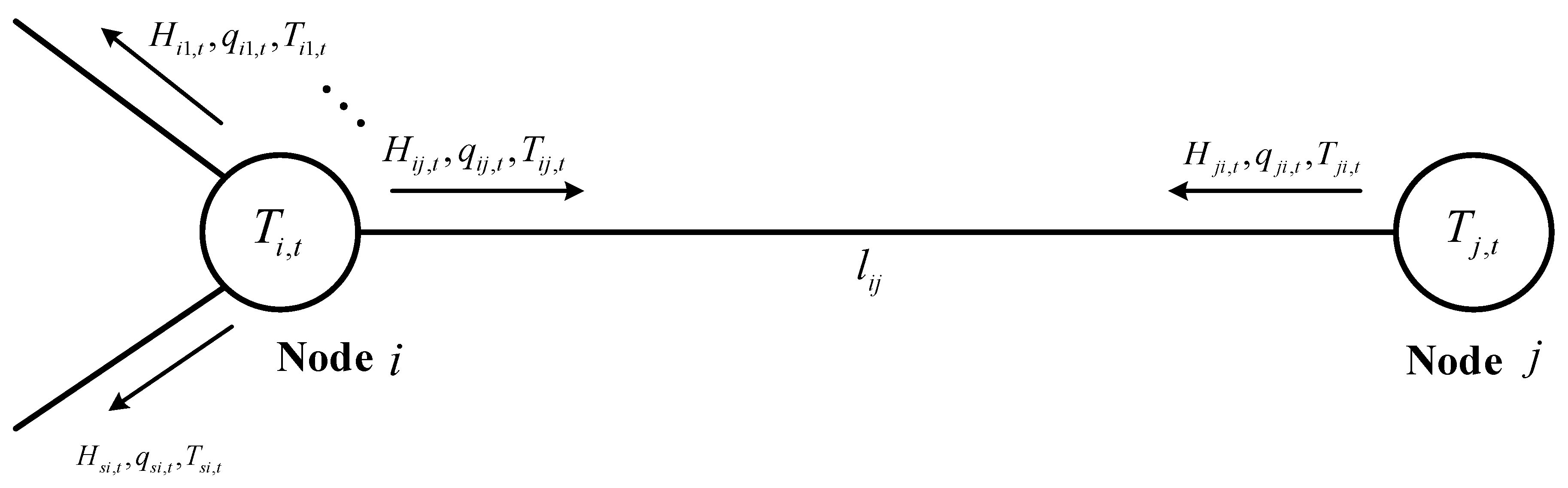
The general model of heat transfer in heating networks is shown in Figure 2. It can be assumed that the connection node between CCHP $i$ and the heating network is marked as node $i$. The heating medium temperature of node $i$, $j$ at time $t$ is $T_{i,t}$ and $T_{j,t}$, respectively, °C. The heating power injected to node $i$ at time $t$ is $H_{si,t}$, kW. The flow rate of heating medium is $q_{si,t}$, m³/s. The temperature is $T_{si,t}$. The heating power of pipeline $i-j$ flowing from node $i$ to node $j$ at time $t$ is $H_{ij,t}$. The flow rate of heating medium is $q_{ij,t}$. The temperature is $T_{ij,t}$. The length of pipeline $i-j$ is $l_{ij}$, km. In the paper, the outflowing heating medium is negative and the inflowing heating medium is positive. As illustrated in Figure 2, the heating network model is mainly composed of two parts: Nodes and the network (pipelines). The node part consists of the flow balance and energy balance. The network part reflects heat loss and transmission time delay.

2.1.1. Pipelines of Heating Networks

The flow process of heating medium in pipelines is accompanied by energy transmission and loss. Based on the basic principle of heat conduction, the heat energy of heating medium in pipeline $i-j$ is:

$$H_{ij,t}=c\rho q_{ij,t}{T}_{ij,t},$$

(1)

where $H_{ij,t}$, $q_{ij,t}$ and $T_{ij,t}$ are the heating power, the mass flow rate and the temperature of the heating medium in pipeline $i-j$ at time $t$, respectively. $c$ is the specific heat capacity of the heating medium, kJ/(kg °C). $\rho$ is the density, $\mathrm{kg}/{\mathrm{m}}^3$.

During heat transfer, the thermal characteristics of heating pipelines have a direct impact on all parts of the heating medium. The thermal characteristics of heating pipelines mainly include the transmission time delay and heat loss [26].

Transmission time delay. The heating medium absorbs heat at the heat source node to increase temperature. Heating mediums transfer to the thermal load side after increasing kinetic energy through circulating water pumps. Therefore, there is a delay effect when the heating medium flows through the pipeline of length $l_{ij}$. The delay time of the temperature change at both ends of pipeline $i-j$ is shown as follows:

$$t_{\mathrm{delay}}=\lceil K_{\mathrm{delay}}\cdot \frac{l_{ij}}{v_t}\rceil ,$$

(2)

where $t_{\mathrm{delay}}$ is the delay time of the heating medium flowing through the pipeline, s. $K_{\mathrm{delay}}$ is the heat delay coefficient, which is related to the laying depth of pipelines. $K_{\mathrm{delay}}$ is 1.39 in the paper [11]. $v_t$ is the velocity of the heating medium in the pipeline at time $t$, m/s. $\lceil ·\rceil$ represents rounding up to an integer.

Heat loss [11]. The heat loss is given by the decrease of the temperature of the heating medium. The heat loss can be solved by Equation (3). Heat loss is a non-linear function related to the temperature of return water. Ignoring the influence of the return water temperature, heat loss can be approximated as follows [10]:

$$\{\begin{array}{l}{H}_{ji,t}=-\left(H_{ij,t-t_{delay}}-\Delta H_{ij,t_{delay}}\right)\\ \Delta H_{ij,t_{delay}}=\frac{T_{ij\mathrm{start},t}-T_{ij\mathrm{out},t}}{T_{ij\mathrm{start},t}-T_{ij\mathrm{return},t}}\left(1-{\mathrm{e}}^{\frac{2\pi \left(T_{ij\mathrm{start},t}-T_{ij\mathrm{return},t}\right)}{H_0{\displaystyle \sum R}}l}\right)\approx \frac{2\pi \left(T_{ij\mathrm{start},t}-T_{ij\mathrm{out},t}\right)}{{\displaystyle \sum R}}{l}_{ij}\end{array}$$

(3)

where $H_{ij,t}$, $H_{ij,t-t_{delay}}$ and $\Delta H_{ij,t_{delay}}$ are thermal load in pipeline $i-j$ at time $t$, thermal power at time $t-t_{delay}$, and the heat loss in time $t_{delay}$. $T_{ij\mathrm{return},t}$ is the temperature of return water. $H_0$ is the thermal power in the pipeline at temperature $T_{ij\mathrm{start},t}$ of the heat source point. ${\displaystyle \sum R}$ is the average thermal resistance between the heating medium and the surrounding environment, km °C/kW.

In addition, considering the corrosion effect and noise pollution of pipelines caused by the rapid flow rate of heating mediums, the flow rate in pipelines needs to meet the following constraints:

$$\left|q_{ij,t}\right|\le v_{ij,t}^{\max }{S}_{ij},$$

(4)

Then,

$$H_{ij,t}^{\max }=c\rho v_{ij,t}^{\max }{S}_{ij}\left(T_{ij\mathrm{start},t}-T_{ij\mathrm{return},t}\right),$$

(5)

where $H_{ij,t}^{\max }$ and $v_{ij,t}^{\max }$ are respectively the maximum thermal power and permissible flow rate of pipeline $i-j$ at time $t$. $S_{ij}$ is the cross-sectional area of pipeline $i-j$, m².

Based on the analysis above, the model of heating networks pipelines can be described as:

$$\{\begin{array}{l}{q}_{ij,t}+q_{ji,t}=0\\ H_{ji,t}=-\left(H_{ij,t-t_{delay}}-\Delta H_{ij,t_{delay}}\right)\\ \Delta H_{ij,t}\le H_{ij,t}\le H_{ij,t}^{\max }\end{array},$$

(6)

The first formula ensures the continuity of heating medium flow. The remaining two formulas represent energy conservation of transmission time delay and heat loss, and the upper and lower limit constraints for thermal power of heating mediums in pipelines.

2.1.2. Nodes of Heating Networks

The node model is composed of the equation of the continuity of mass flow equation, and the mixture of node temperatures equation.

The equation of the continuity of mass flow is that the sum of inflow mass flow is equal to the sum of outflow mass flow at each node. Specifically, it can be characterized by the following formula:

$${\displaystyle \sum _{i\in S^{\mathrm{in}}}{q}_{t-t_{\mathrm{delay}}}}+{\displaystyle \sum _{i\in S^{\mathrm{out}}}{q}_t}=0$$

(7)

The equation of the mixture of node temperatures considers heating mediums at node i. Then,

$$T_{i\mathrm{mix},t}=\frac{\left(c\rho {\displaystyle \sum _{i\in S^{\mathrm{in}}}{q}_{t-t_{\mathrm{dealy}}}{T}_{t-t_{\mathrm{delay}}}}\right)-{\displaystyle \sum _{i\in S^{\mathrm{in}}}\Delta H_{t_{\mathrm{delay}}}}}{c\rho {\displaystyle \sum _{i\in S^{\mathrm{out}}}{q}_t}},$$

(8)

where $S^{\mathrm{in}}$ and $S^{\mathrm{out}}$ are pipeline sets for inflow and outflow joints of heating mediums, respectively. $q_{t-t_{\mathrm{dealy}}}$ and $T_{t-t_{\mathrm{delay}}}$ are the heating medium flow and temperature at time $t-t_{\mathrm{delay}}$. $q_t$ is the flow rate of outflowing heating medium. $T_{i\mathrm{mix},t}$ is the temperature of mixed heating mediums at node $i$.

2.2. Coupling Structure of Heating Networks and Multi-District IES

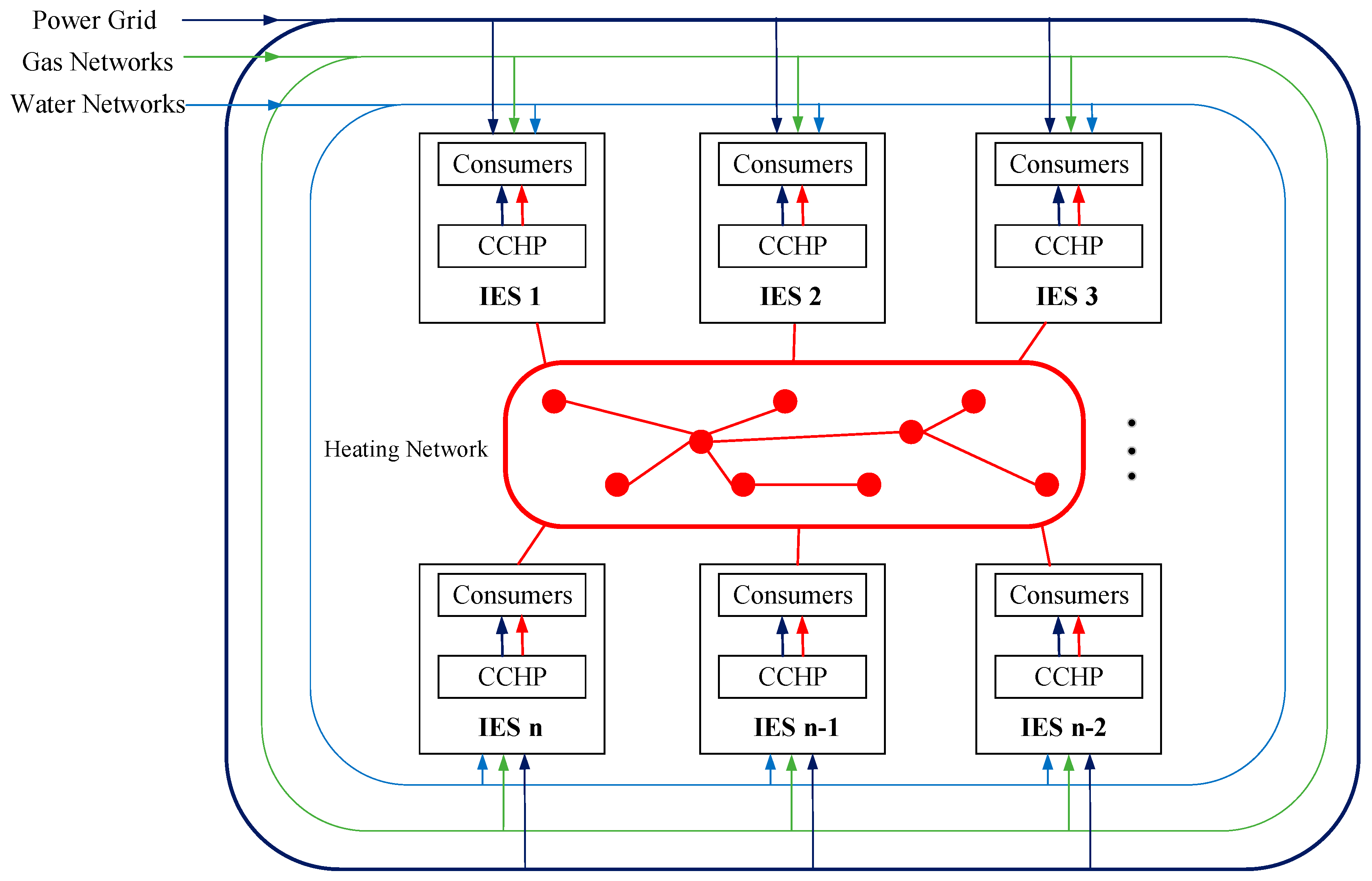
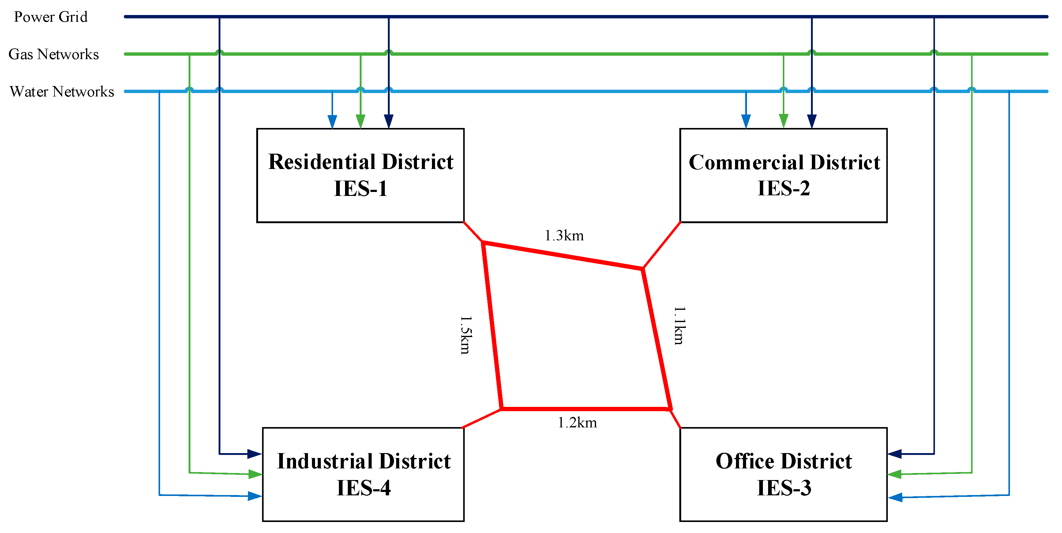
The structure of interconnected system for multi-district IES studied in this paper is shown in Figure 3. The system is mainly composed of CCHP system, power grid, heating network, and gas network in different IES districts. CCHP gives surplus electricity to the power grid when it is permitted by dispatching operators. The thermal power between IES in each district can be transferred to each other through the heating network. The excess heat energy in the district with abundant heat energy supply can be transferred to other districts.

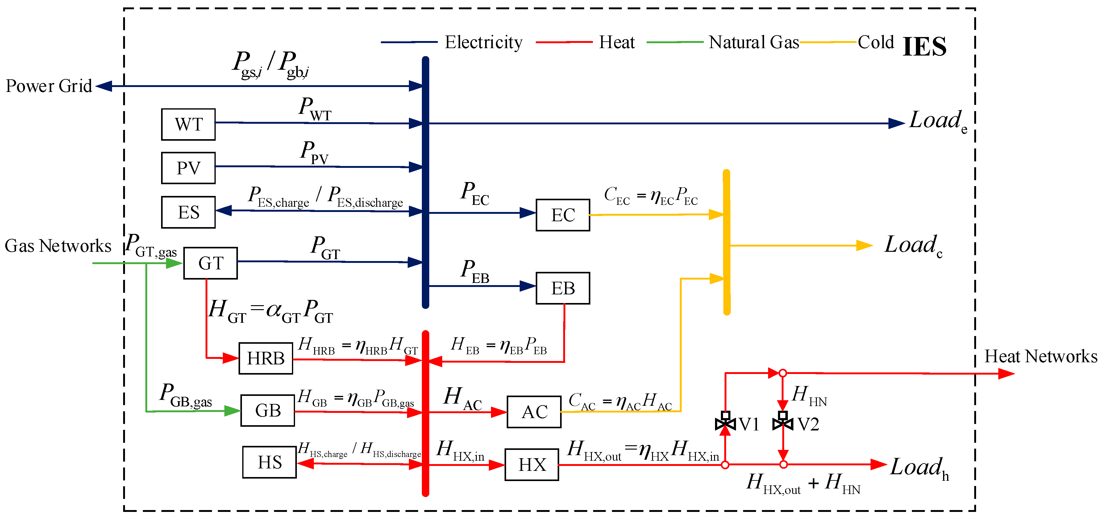
As shown in Figure 4, the thermal power transmission of the CCHP system is bidirectional. The bidirectional selectivity of the coupling link is realized through the automatic control of valve V1 and V2 [10]. When V1 is opened and V2 is closed, thermal power is transmitted to the heating network and connect with thermal load. When V1 is closed and V2 is opened, the heating network and CCHP system is able to connect with thermal load together. The flow of electric, thermal and cold power, and their calculation methods can be obtained from Figure 4.

The main equipment in IES include heat recovery boiler (HRB), heat exchange device (HX), micro gas turbine (GT), gas boiler (GB), electric boiler (EB), absorption cooler (AC), electric cooler (EC), electric energy storage (ES) and heat energy storage (HS), wind turbine (WT), photovoltaic unit (PV). The model is detailed in [2,3].

3. Flexible Demand Response of Electric and Thermal Load

The FDR in this paper is realized by adjusting flexible electric load and flexible thermal load. Flexible electric load in IES adopts shiftable load. Thermal load includes heating load and hot water load. The FDR is based on the two-dimensional controllability of time and space. The time controllability is realized by adjusting the shiftable electric load and heating load in the operation dispatching. The space controllability is realized by the comfortable fuzziness from shiftable electric load and heating load.

3.1. FDR Analysis of Shiftable Electric Load

Residential consumers, industrial consumers, commercial consumers, and office consumers all have certain shiftable loads. Residential consumers can transfer load by adjusting the time of household appliances, such as using washing machines, dishwashers, water heaters in the valley period. Industrial consumers with shiftable load can be divided into three categories [27]: (a) High-energy-consuming enterprises are the main contributors of shiftable loads because of their large power consumption. Under the appropriate DR incentive, they can arrange most of their production at night. (b) Metallurgical, mechanical and textile enterprises with three shifts. The production task of the industry is continuous, so it only needs to transfer part load within a certain time without affecting the overall production process to realize peak avoidance. For example, the cement industry can carry out grinding operation in the valley period, while the raw materials of the storage bin are used in the peak period. However, the capacity of such enterprises to transfer load is limited. (c) Private and individual enterprises with flexible management can adjust their transferable loads freely because of flexible management, but their electricity consumption is relatively small.

Due to the industry nature of commercial consumers and office consumers, they are not able to transfer much load. However, they still have the potential of load transfer.

After the implementation of FDR of electric load, the load in each period is the original load plus the increasing load, and then the reduced load is subtracted, as given in Equation (9).

$$Loa{d}_{\mathrm{e},i,t}^{\mathrm{new}}=Loa{d}_{\mathrm{e},i,t}^{\mathrm{old}}+Loa{d}_{\mathrm{e},i,t}^{\mathrm{u}}-Loa{d}_{\mathrm{e},i,t}^{\mathrm{d}},$$

(9)

Where ${Load}_{e,i,t}^{\mathrm{old}}$ and ${Load}_{e,i,t}^{\mathrm{new}}$ are respectively total load demands before and after FDR implementation. ${Load}_{e,i,t}^{\mathrm{u}}$ and ${Load}_{e,i,t}^{\mathrm{d}}$ are respectively load increment and load reduction of consumer i at time t.

Usually, the total load demand depends on the household demand and production task. In the way of load transfer, consumers do not need to reduce the household demand or interrupt the production task. They can change the using time of electric energy and keep the total power consumption constant in the cycle, so the household demand and the total output are not affected. According to previous studies, there are two limitations on increasing and reducing load demand. (a) In a cycle (especially within a working day), the total power consumption remains unchanged. Load increment and reduction need to be balanced. (b) Any user has a certain uncontrollable basic load, and only part load can be adjusted. There are certain restrictions on the load increment and reduction in each time. It can be expressed as the following formula:

$$\{\begin{array}{l}{\displaystyle \sum _{i=1}^N{\displaystyle \sum _{t=1}^{M}Loa{d}_{\mathrm{e},i,t}^{\mathrm{u}}}}={\displaystyle \sum _{i=1}^N{\displaystyle \sum _{t=1}^{M}Loa{d}_{\mathrm{e},i,t}^{\mathrm{d}}}}\\ 0\le Loa{d}_{\mathrm{e},i,t}^{\mathrm{u}}\le Loa{d}_{\mathrm{e},i,t}^{\mathrm{umax}}\\ 0\le Loa{d}_{\mathrm{e},i,t}^{\mathrm{d}}\le Loa{d}_{\mathrm{e},i,t}^{\mathrm{dmax}}\end{array},$$

(10)

where N is the number of consumers. M is the total number of time periods in the scheduling cycle. ${Load}_{e,i,t}^{\mathrm{umax}}$ and ${Load}_{e,i,t}^{\mathrm{dmax}}$ are the maximum allowable load increment and reduction of consumer i at time t, respectively.

3.2. FDR Analysis of Thermal Load

The main demand of thermal system is heating load in winter. Taking heating load model as an example, a flexible thermal load model is established.

$$Q_{\mathrm{h},t}=\frac{C_{\mathrm{h}}{S}_{\mathrm{h}}}{\Delta t}\left(T_{\mathrm{in},t}-T_{\mathrm{in},t-1}\right)+\mu S_{\mathrm{h}}\left(T_{\mathrm{in},t}-T_{\mathrm{out},t}\right),$$

(11)

where Q_h,t is the heating load at time t, kW. T_in,t and T_out,t are respectively indoor and outdoor temperatures at time t. C_h is the heat capacity of per unit heating area, which is taken as 0.08 kW/m²℃ in the paper. S_h is the heating area, m². μ is the indoor heat loss per unit temperature difference and unit heating area, which is taken as 0.04 kW/m² °C.

The indoor temperature is an important index affecting heating load. The restriction of consumer’s thermal comfort is the restriction of temperature range.

$$\{\begin{array}{l}{T}_t^{\min }=T_{\mathrm{mid},t}-\Delta T^{\max }/2\\ T_t^{\max }=T_{\mathrm{mid},t}+\Delta T^{\max }/2\\ T_{\mathrm{in},t}=T_{\mathrm{in},t-1}+\Delta T_{\mathrm{in},t}\\ \left|\Delta T_{\mathrm{in},t}\right|\le \Delta T^{\max }\end{array},$$

(12)

where $T_t^{\max }$ and $T_t^{\min }$ are respectively the upper and lower adjusting range of indoor temperature. T_mid,t is the middle value of setting temperature range [$T_t^{\min }$, $T_t^{\max }$]. ∆T_in,t is the changing value of indoor temperature. ∆T^max is the maximum setting variable quantity of indoor temperature.

Equation (13) establishes a dynamic model of heating load, and indoor and outdoor temperature. Since the thermal load has time continuity and the indoor heating comfort demand of Equation (12) restricts the amount of temperature change at adjacent time, it is necessary to calculate the amount of thermal load change caused by the temperature difference of adjacent time. The relationship between the difference of indoor and outdoor temperature ∆T_t,t−1 = T_in,t − T_in,t−1 and real-time change of heat consumption ∆ Q_h,t is as follows:

$$\Delta Q_{\mathrm{h},t}=f\left(\Delta T_{t,t-1}\right)=f\left(T_{\mathrm{in},t}-T_{\mathrm{in},t-1}\right),$$

(13)

where ∆T_t,t−1 is the temperature difference between time t and time t−1. ∆ Q_h,t is the difference of heat consumption of time t and time t−1.

Equations (13) and (14) can be used to calculate the indoor heat demand at different temperatures.

$$\Delta Q_{\mathrm{h},{\mathrm{T}}_{\mathrm{n}}}=f\left({\mathrm{T}}_{\mathrm{n}}\right)-f\left({\mathrm{T}}_{\mathrm{n}}-m\right),$$

(14)

where ∆ Q_h,Tn is the heat required to raise indoor temperature by m °C.

Load characteristics of the thermal system has the following load characteristics. Firstly, temperature is its regulation scale with a low consumer’s sensitivity, so temperature only needs to be assured in the comfort zone. Secondly, affected by the regulation means and network characteristics, thermal system has a slow regulation rate relative to power system dispatching. The building envelope and network structure have a certain heat storage capacity, which makes it strong enough to suppress and tolerate short-term fluctuations and intermittences. Flexible thermal load regulation is as follows:

$$P_{\mathrm{h},t}^{\mathrm{FDR}}={\alpha }_{\mathrm{h},t}^{\mathrm{FDR}}{H}_t^{\mathrm{FDR},\max },{\alpha }_{\mathrm{h},t}^{\mathrm{FDR}}\in [0,1],$$

(15)

where $P_{\mathrm{h},t}^{\mathrm{FDR}}$ is the controlled quantity of thermal load. ${\alpha }_{\mathrm{h},t}^{\mathrm{FDR}}$ is the regulation rate. ${\alpha }_{\mathrm{h},t}^{\mathrm{FDR}}$ > 0 indicates that the regulation is in progress and ${\alpha }_{\mathrm{h},t}^{\mathrm{FDR}}$ = 0 indicates that the regulation is interrupted. $H_t^{\mathrm{FDR},\max }$ represents the maximum FDR controlled quantity of thermal load at time t. FDR dispatch of thermal system should satisfy the constraints of consumer’s comfort, which needs to constrain the regulating range of indoor temperature. The maximum constraints of FDR regulation can be calculated by Equations (14) and (15).

$$P_{\mathrm{h},t}^{\mathrm{FDR}}\le \Delta Q_t^{\mathrm{FDR},\max },$$

(16)

where ∆$Q_t^{\mathrm{FDR},\max }$ is the maximum controlled quantity under temperature constraints, which can be calculated by Equations (13)–(15).

The DR of thermal load is to increase the controlled quantity as much as possible and promote the flexible adjustment ability of thermal load under the condition of satisfying the consumer’s satisfaction and the controlled restriction of thermal load. In this paper, the calculation method of adjustment cost for thermal load is given by:

$$C_{\mathrm{h}}^{\mathrm{FDR}}={\displaystyle \sum _{i=1}^N{\displaystyle \sum _{t=1}^M{b}_{\mathrm{h}}^{\mathrm{FDR}}{P}_{\mathrm{h},i,t}^{\mathrm{FDR}}}},$$

(17)

where $C_{\mathrm{h}}^{\mathrm{FDR}}$ is the compensation cost for thermal load FDR. $b_{\mathrm{h}}^{\mathrm{FDR}}$ is the compensation unit price. $P_{\mathrm{h},i,t}^{\mathrm{FDR}}$ is the regulation amount of thermal load of IES i at time t. Based on Weber-Fechner law, this paper constructs a model of consumers’ willingness to participate in FDR of thermal load. Through the empirical calculation of this law, a more reasonable and effective pricing scheme is proposed to meet the psychological expectation. Therefore, the relationship between the real-time compensation price of FDR and real-time electricity price is as follows:

$$b_{\mathrm{h}}^{\mathrm{FDR}}=b_{\mathrm{h}}\ln \left(c_{\mathrm{h}}\right)+C,$$

(18)

where b_h is the compensation coefficient of thermal load FDR, whose value is 0.5. c_h is the selling price of thermal load, the value is 0.8.

4. Operation Optimization Model of Multi-District IES Considering FDR of Electric and Thermal Load

The optimization of the coupled system of heating network and multi-district IES is based on the power constraints, operation constraints of heating networks, and main equipment. Considering the FDR control of electric and thermal power, an economic optimal dispatching model for multi-district IES is proposed.

4.1. Objective Function

The optimization objective function includes the cost of purchasing electricity from the power grid, the profit of selling electricity to the power grid, the natural gas cost, the operation cost of the heating network and the compensation cost of FDR for thermal load. The formula is as follows:

$$\min C_{\mathrm{MD-IES}}=C_{\mathrm{e},\mathrm{b}}-C_{\mathrm{e},\mathrm{s}}+C_{\mathrm{gas}}+C_{\mathrm{HN}}+C_{\mathrm{h}}^{\mathrm{FDR}},$$

(19)

where C_e,b, C_e,s, C_gas C_HN and $C_{\mathrm{h}}^{\mathrm{FDR}}$ are the cost of purchasing electricity from the power grid, the profit of selling electricity to the power grid, the natural gas cost, the operation cost of the heating network, and the compensation cost of FDR for thermal load, respectively, ¥.

$$C_{\mathrm{e},\mathrm{b}}={\displaystyle \sum _{i=1}^N{\displaystyle \sum _{t=1}^M\left(c_{\mathrm{e},\mathrm{b},t}{P}_{\mathrm{g},\mathrm{b},i,t}\Delta t\right)}},$$

(20)

where N is the number of districts in multi-district IES. M is the total number of scheduling periods. c_e,b,t is the purchase price of electricity at time t, ¥/(kWh). P_g,b,i,t is the power purchased from the grid of district i at time t, kW. ∆t is time of each scheduling period, h.

$$C_{\mathrm{e},\mathrm{s}}={\displaystyle \sum _{i=1}^N{\displaystyle \sum _{t=1}^M\left(c_{\mathrm{e},\mathrm{s},t}{P}_{\mathrm{g},\mathrm{s},i,t}\Delta t\right)}},$$

(21)

where c_e,s,t is the unit price of selling electricity, ¥/(kWh). P_g,b,i,t is the power sold to the grid, kW.

The natural gas cost is as follows:

$$C_{\mathrm{gas}}=c_{\mathrm{gas}}{\displaystyle \sum _{i=1}^N{\displaystyle \sum _{t=1}^M\left(P_{\mathrm{GT},\mathrm{gas},i,t}+P_{\mathrm{GB},\mathrm{gas},i,t}\right)}}\Delta t=c_{\mathrm{gas}}{\displaystyle \sum _{i=1}^N{\displaystyle \sum _{t=1}^M\left(\frac{P_{\mathrm{GT},i,t}}{{\eta }_{\mathrm{GT},i}}+\frac{Q_{\mathrm{GB},i,t}}{{\eta }_{\mathrm{GB},\mathrm{i}}}\right)}}\Delta t,$$

(22)

where c_gas is the unit calorific value price of natural gas, ¥/(kWh). P_GT,gas,i,t and P_GB,gas,i,t are respectively the electric and thermal power of GT and GB in district i at time t, kW. ${\eta }_{GT,i}$ and ${\eta }_{GB,i}$ are respectively the efficiencies of GT and GB in district i.

The operation cost of the heating network is mainly the electricity cost of circulating pumps in pipelines, which can be estimated by ratios of electricity consumption to transfer heat quantity [28].

$$C_{\mathrm{HN}}={\displaystyle \sum _{i=1}^R{\displaystyle \sum _{t=1}^M\left(EH{R}_i{c}_{\mathrm{e},\mathrm{b},t}{H}_{\mathrm{HN},i,t}\Delta t\right)}},$$

(23)

where R is the number of circulating pumps. EHR_i is the ratio of electricity consumption to transfer heat quantity of pump i. H_HN,i,t is the heat distributed by pump i, kW.

The formula for calculating the compensation cost of FDR of thermal load is shown in Equation (17).

4.2. Operation Constraints

For the IES structure shown in Figure 4, the constraints mainly include the energy balance constraints of the electric, thermal, and cooling bus, the output constraints of CCHP system in multi-district IES, the FDR constraints, the heating network constraints and the coupling constraints of the heating network and multi-district IES.

Considering the affiliated status of energy conversion devices and the diversity of energy conversion forms, relevant literature usually merge energy conversion devices into source equipment with energy efficiency when modeling CCHP system [29]. In this paper, the bus structure is adopted, which can independently model different power sources, thermal sources, energy storages, conversion devices for electric, thermal, and cooling loads. At the same time, it is easy to write system equilibrium equations and equipment constraints.

4.2.1. Energy Balance Constraints of Bus

The balance equation of electric bus is as follows:

$$P_{\mathrm{g},\mathrm{b},i,t}-P_{\mathrm{g},\mathrm{s},i,t}+P_{\mathrm{WT},i,t}+P_{\mathrm{PV},i,t}+P_{\mathrm{ES},\mathrm{discharge},i,t}-P_{\mathrm{ES},\mathrm{charge},i,t}+P_{\mathrm{GT},i,t}=Loa{d}_{\mathrm{e},i,t}^{\mathrm{new}}+P_{\mathrm{EC},i,t}+P_{\mathrm{EB},i,t},$$

(24)

where P_g,b,i,t and P_g,s,i,t are respectively the purchasing and selling electric power with the superior power grid of district i at time t. P_WT,i,t, P_PV,i,t, P_{ES,discharge,i,t}, P_{ES,charge,i,t} and P_GT,i,t are the outputs of WT and PV, the charging and discharging power of ES, and the output of GT of district i at time t. ${Load}_{e,i,t}^{\mathrm{new}}$, P_EC,i,t and P_EB,i,t are the electric load, the power of EC and EB, respectively.

The balance equation of thermal bus is as follows:

$${\eta }_{\mathrm{HRB},i}{\alpha }_{\mathrm{GT},i}{P}_{\mathrm{GT},i,t}+{\eta }_{\mathrm{GB},i}{P}_{\mathrm{GB},\mathrm{gas},i,t}+{\eta }_{\mathrm{EB},i}{P}_{\mathrm{EB},i,t}+H_{\mathrm{HS},\mathrm{disch}\arg \mathrm{e},i,t}-H_{\mathrm{HS},\mathrm{ch}\arg \mathrm{e},i,t}=H_{\mathrm{AC},i,t}+H_{\mathrm{HX},\mathrm{in},i,t},$$

(25)

where ${\eta }_{\mathrm{HRB},i}$, ${\eta }_{\mathrm{GB},i}$, ${\eta }_{\mathrm{EB},i}$ and ${\alpha }_{\mathrm{GT},i}$ are the transformation efficiencies of HRB, GB, and EB, and the heat-to-electric ratio of GT in district i, respectively. P_GBgas,i,t, H_{HS,discharge,i,t}, H_{HS, charge,i,t}, H_AC,i,t and H_HX,in,i,t are natural gas consumed by GB, releasing and storing thermal power of HS, thermal power consumed by AC and HX in district i at time t, respectively.

The balance equation of cooling bus is as follows:

$${\eta }_{\mathrm{EC},i}{P}_{\mathrm{EC},i,t}+{\eta }_{\mathrm{AC},i}{H}_{\mathrm{AC},i,t}=Loa{d}_{\mathrm{c},i,t},$$

(26)

where ${\eta }_{\mathrm{EC},i}$ and ${\eta }_{\mathrm{AC},i}$ are the transformation efficiencies of EC and AC. Load_c,i,t is the cooling load in district i at time t.

4.2.2. Output Constraints of CCHP System in Multi-District IES

In addition to the bus energy balance equation of the system, the constraints of various types of equipment including the upper and lower output limits, charging and discharging power and energy constraints of energy storage equipment should also be considered.

The electrical, thermal, and cooling power of each equipment meets the requirements of upper and lower limits:

$$\{\begin{array}{l}{P}_i^{\min }\le P_i\le P_i^{\max }\\ H_i^{\min }\le H_i\le H_i^{\max }\\ C_i^{\min }\le C_i\le C_i^{\max }\end{array},$$

(27)

where P_i, H_i and C_i are electrical, thermal, and cooling power of equipment i, respectively. $P_i^{\min }$, $P_i^{\max }$, $H_i^{\min }$, $H_i^{\max }$, $C_i^{\min }$ and $C_i^{\max }$ are the lower and upper limits of electrical, thermal, and cooling power of equipment i, respectively.

For energy storage equipment, the operation constraints include charging and discharging power, storage energy and other constraints.

$$\{\begin{array}{l}0\le P_{\mathrm{ES},\mathrm{charge},i,t}\le {\gamma }_{\mathrm{ES},\mathrm{charge},i}^{\max }Ca{p}_{\mathrm{ES},i}\\ 0\le P_{\mathrm{ES},\mathrm{discharge},i,t}\le {\gamma }_{\mathrm{ES},\mathrm{discharge},i}^{\max }Ca{p}_{\mathrm{ES},i}\\ P_{\mathrm{ES},\mathrm{charge},i,t}{P}_{\mathrm{ES},\mathrm{discharge},i,t}=0\\ E_{\mathrm{ES},i,t}=\left(1-{\sigma }_{\mathrm{ES},i}\right)E_{\mathrm{ES},i,t-1}+\left({\eta }_{\mathrm{ES},\mathrm{ch}\arg \mathrm{e},i}{P}_{\mathrm{ES},\mathrm{charge},i,t}+\frac{P_{\mathrm{ES},\mathrm{discharge},i,t}}{{\eta }_{\mathrm{ES},\mathrm{disch}\arg \mathrm{e},i}}\right)\Delta t\\ E_{\mathrm{ES},i}^{\min }\le E_{\mathrm{ES},i,t}\le E_{\mathrm{ES},i}^{\max }\\ E_{\mathrm{ES},i,0}=E_{\mathrm{ES},i,\mathrm{T}}\end{array},$$

(28)

where ${\gamma }_{\mathrm{ES},\mathrm{charge},i}^{\max }$ and ${\gamma }_{\mathrm{ES},\mathrm{discharge},i}^{\max }$ are respectively the maximum ratios of charging and discharging of ES i. The third formula guarantees charging and discharging are not at the same time. E_ES,i,t is the stored energy of ES i at time t, kWh. Cap_ES,i is the maximum capacity of ES i, kWh. ${\sigma }_{\mathrm{ES},\mathrm{i}}$, ${\eta }_{\mathrm{ES},\mathrm{charge},i}$ and ${\eta }_{\mathrm{ES},\mathrm{discharge},i}$ are respectively the self-discharge rate, and efficiencies of charging and discharging of ES i. $E_{\mathrm{ES},i}^{\max }$ and $E_{\mathrm{ES},i}^{\min }$ are respectively the maximum and minimum stored energy of ES i. The fifth formula indicates that the stored energy remains unchanged before and after the scheduling cycle.

The FDR constraints are detailed in Equations (9)–(16). The constraints of the heating network are detailed in Equation (6).

4.2.3. Coupling Constraints of the Heating Network and Multi-District IES

Compared with IES without heating networks, multi-district IES with DHN adds the energy coupling link between CCHP system and the heating network at the output port of HX. The corresponding coupling constraint is the energy coupling equation as follows:

$$H_{\mathrm{HX},\mathrm{out},i,t}+H_{\mathrm{HN},i,t}=Loa{d}_{\mathrm{h},i,t},$$

(29)

where, H_HX,out,i,t H_HN,i,t and Load_h,i,t are the thermal power of HX, thermal power obtained from the heating network and thermal load of the system.

The optimization model consists of three parts: The optimization of energy flow in each IES district, FDR control for electric and thermal load, and energy flow paths in the heating network. They are coupled through thermal power between multi-district IES and the heating network.

4.3. Model Solution

In this paper, a 0–1 MILP method is used to solve the optimization model. The standard form of the model is as follows:

$$\{\begin{array}{ll}\min & {\mathit{c}}^{\mathrm{T}}\mathit{x}\\ \mathrm{s}.\mathrm{t}.& \mathit{A}\mathit{x}=\mathit{b}\\ & x_{\min }\le x_i\le x_{\max },& i\in \mathit{I}\\ & x_j\in \left\{0,1\right\},& j\in \mathit{J}\end{array},$$

(30)

The decision variables include the output of CCHP units in each district, the real-time storing and releasing power of electric and thermal energy storage devices, the purchasing and selling electricity with the power grid, the output of conversion equipment and the thermal power flow in the pipelines of the heating network. Equality constraints and inequality constraints are shown in

Table 1. Details of constraints.

Constraints Type	IES	FDR	Heating Networks	Coupling Relation
Equality constraints	① Energy balance equation of bus ② Energy relationship of energy storage devices ③ Energy conversion relationship of CCHP system	① Equation constraints of electric load	① Equilibrium equation of node ② Heat loss equation of pipelines	① Energy coupling equation of the heating network and CCHP system
Inequality constraints	① Operating constraints of CCHP system ② Power constraints of energy storage devices	① Flexible control constraints of thermal load	① Input and output power constraints of pipelines	Null

. Since the constraints include coupling variables, such as the storing and releasing power of electric and thermal energy storage devices, and the purchasing and selling electricity, the 01 variable is introduced into the model.

At present, there are mature algorithms to solve the model, which can be directly solved by commercial software such as Cplex, Gurobi, Lingo, etc. Based on Yalmip and Cplex tool in MATLAB 2015a, a 0–1 MILP program is developed to solve the problem in the paper.

5. Case Analysis

5.1. Case Description

In this paper, the coupled system of multi-district IES with DHN is taken as a case as shown in Figure 5. The IES is divided into four sub-districts: Residential district, commercial district, office district, and industrial district. The CCHP system is built in each district. The CCHP system structure for each sub-district is shown in Figure 4. Electric and thermal energy storage devices are equipped in each district. The capacity of each equipment is shown in

Table 2. Capacities of devices in each sub-district.

Devices	Capacities of Devices/(kW)
	IES-1	IES-2	IES-3	IES-4
WT	1000	2500	1600	5000
PV	500	1200	1000	2000
GT	2000	8000	3000	15,000
HRB	5000	15,000	8000	30,000
GB	5000	5000	5000	10,000
EB	5000	5000	5000	10,000
HX	10,000	20,000	10,000	40,000
EC	5000	5000	5000	10,000
AC	5000	5000	5000	10,000
Devices	Capacities of Devices/(kWh)
	IES-1	IES-2	IES-3	IES-4
ES	1000	1000	1000	2000
HS	2000	2000	2000	6000

. The parameters of the heating network are given in

Table 3. Parameters of the heating network.

Pipeline	Length/(km)	Diameter/(m)	Maximum Flow Velocity/(m/s)	∑R/(km·°C/kW)	EHR
1-2	1.3	0.3	3	20	0.0063
2-3	1.1	0.3	3	20	0.0059
3-4	1.2	0.3	3	20	0.0069
4-1	1.5	0.3	3	20	0.0058

. The running cost of the heating network in the simulation is calculated according to the thermal power distributed by pipelines. Detailed equipment parameters in each sub-districts are given in

Table 4. Equipment parameters of IES in each sub-district.

Parameters	IES-1	IES-2	IES-3	IES-4
$P_{\mathrm{GT}}^{\min }$/(kW)	120 or OFF	450 or OFF	200 or OFF	800 or OFF
${\alpha }_{\mathrm{GT}}$	2.3	2.3	2.3	2.3
${\eta }_{\mathrm{GT}}$	0.3	0.3	0.3	0.3
${\eta }_{\mathrm{HRB}}$	0.73	0.73	0.73	0.73
${\eta }_{\mathrm{GB}}$	0.9	0.9	0.9	0.9
${\eta }_{\mathrm{EB}}$	0.9	0.9	0.9	0.9
${\eta }_{\mathrm{EC}}$	4	4	4	4
${\eta }_{\mathrm{AC}}$	1.2	1.2	1.2	1.2
${\eta }_{\mathrm{HX}}$	0.9	0.9	0.9	0.9
${\gamma }_{\mathrm{ES},\mathrm{charge}}^{\max }$	0.2	0.2	0.2	0.2
${\gamma }_{\mathrm{ES},\mathrm{discharge}}^{\max }$	0.4	0.4	0.4	0.4
${\eta }_{\mathrm{ES},\mathrm{ch}\arg \mathrm{e}}$	0.95	0.95	0.95	0.95
${\eta }_{\mathrm{ES},\mathrm{disch}\arg \mathrm{e}}$	0.95	0.95	0.95	0.95
${\sigma }_{\mathrm{ES}}$	0.04	0.04	0.04	0.04
$E_{{}_{\mathrm{ES}}}^{\max }/Ca{p}_{\mathrm{ES}}$	0.9	0.9	0.9	0.9
$E_{{}_{\mathrm{ES}}}^{\max }/Ca{p}_{\mathrm{ES}}$	0.2	0.2	0.2	0.2
${\gamma }_{\mathrm{HS},\mathrm{charge}}^{\max }$	0.2	0.2	0.2	0.2
${\gamma }_{\mathrm{HS},\mathrm{discharge}}^{\max }$	0.4	0.4	0.4	0.4
${\eta }_{\mathrm{HS},\mathrm{ch}\arg \mathrm{e}}$	0.95	0.95	0.95	0.95
${\eta }_{\mathrm{HS},\mathrm{disch}\arg \mathrm{e}}$	0.95	0.95	0.95	0.95
${\sigma }_{\mathrm{HS}}$	0.1	0.1	0.1	0.1
$E_{{}_{\mathrm{HS}}}^{\max }/Ca{p}_{\mathrm{ES}}$	0.9	0.9	0.9	0.9
$E_{{}_{\mathrm{HS}}}^{\max }/Ca{p}_{\mathrm{ES}}$	0.1	0.1	0.1	0.1

.

The time-of-use tariff is used for residential and industrial users in the example as shown in Appendix A (

Table A1. Time-of-use electricity price.

Area	Category	Concrete Time	Price/(¥/kWh)
Resident	Peak period	12:00~16:00,19:00~22:00	0.89
Industry		9:00~13:00,18:00~22:00	1.435
Resident	Normal period	8:00~12:00,16:00~19:00,22:00~24:00	0.49
Industry		13:00~18:00,22:00~24:00	0.861
Resident	Valley period	0:00~8:00	0.25
Industry		0:00~9:00	0.387

). Fixed tariffs are adopted for both commercial and office districts, both of which are 0.882 ¥/kWh. IES sells electricity to the power grid at the price of 0.61 ¥/kWh and the converted natural gas at a calorific value of 0.29 ¥/kWh, so $b_{\mathrm{h}}^{\mathrm{FDR}}=0.18\yen /\left(\mathrm{kWh}\right)$. The maximum power point tracking mode is used for WT and PV. The real-time outputs of WT and PV are shown in

Table A2. Forecast outputs of WT and PV.

Time	Forecast Outputs of WT/(kW)				Forecast Outputs of PV/(kW)
	Resident	Commerce	Office	Industry	Resident	Commerce	Office	Industry
00:00~01:00	525	1837.5	1050	4200	0	0	0	0
01:00~02:00	545	1907.5	1090	4360	0	0	0	0
02:00~03:00	495	1732.5	990	3960	0	0	0	0
03:00~04:00	450	1575	900	3600	0	0	0	0
04:00~05:00	427.5	1496.25	855	3420	0	0	0	0
05:00~06:00	375	1312.5	750	3000	0	0	0	0
06:00~07:00	255	892.5	510	2040	61.8	255	139.2	507.6
07:00~08:00	137.5	481.25	275	1100	110.4	458.4	252	914.4
08:00~09:00	200	700	400	1600	160.2	661.8	363	1320
09:00~10:00	200	700	400	1600	184.8	763.2	417	1523.4
10:00~11:00	275	962.5	550	2200	209.4	865.8	474	1726.8
11:00~12:00	335	1172.5	670	2680	234	966	531	1932
12:00~13:00	220	770	440	1760	246	990	558	2032.2
13:00~14:00	242.5	848.75	485	1940	246	990	558	2032.2
14:00~15:00	162.5	568.75	325	1300	234	966	528	1930.2
15:00~16:00	232.5	813.75	465	1860	196.8	814.8	447	1625.4
16:00~17:00	275	962.5	550	2200	147.6	611.4	336	1219.2
17:00~18:00	335	1172.5	670	2680	73.8	306	168	609.6
18:00~19:00	397.5	1391.25	795	3180	0	0	0	0
19:00~20:00	442.5	1548.75	885	3540	0	0	0	0
20:00~21:00	460	1610	920	3680	0	0	0	0
21:00~22:00	485	1697.5	970	3880	0	0	0	0
22:00~23:00	522.5	1828.75	1045	4180	0	0	0	0
23:00~24:00	542.5	1898.75	1085	4340	0	0	0	0

. Electrical, thermal, and cooling loads in different districts are detailed in

Table A3. Electric and thermal load.

Time	Electric load/(kW)				Thermal Load/(kW)
	Resident	Commerce	Office	Industry	Resident	Commerce	Office	Industry
00:00~01:00	1200	2200	800	3000	3600	0	0	7000
01:00~02:00	1200	2200	800	3000	3600	0	0	7000
02:00~03:00	1200	2200	800	3000	3600	0	0	7000
03:00~04:00	1200	2200	800	3000	3600	0	0	7000
04:00~05:00	1200	2200	800	3000	3600	0	0	7000
05:00~06:00	1200	2200	800	3000	3600	0	0	7000
06:00~07:00	1200	2200	800	3000	3600	0	0	7000
07:00~08:00	1600	2200	800	3000	3600	0	0	7000
08:00~09:00	2000	6400	2000	3000	4000	1800	2400	7000
09:00~10:00	2400	7200	4400	9000	4200	2800	4200	25,000
10:00~11:00	2800	7600	4400	9000	4200	3600	4400	25,000
11:00~12:00	2400	7600	4400	9000	4200	4000	4200	25,000
12:00~13:00	2400	7600	4400	9000	4000	4400	4000	25,000
13:00~14:00	2400	7800	4400	9000	3600	4000	4000	25,000
14:00~15:00	2400	8000	4400	9000	3600	4000	4000	25,000
15:00~16:00	2800	8000	4400	9000	3600	4000	4000	25,000
16:00~17:00	2800	7600	4400	9000	3600	4000	4000	25,000
17:00~18:00	2800	7200	2000	9000	4000	4200	4000	25,000
18:00~19:00	2800	6400	1200	3000	4200	4200	2000	7000
19:00~20:00	2800	6400	800	3000	4200	4000	1000	7000
20:00~21:00	2400	6400	800	3000	4200	3600	500	7000
21:00~22:00	2000	5200	800	3000	4000	2800	0	7000
22:00~23:00	1600	2200	800	3000	3600	0	0	7000
23:00~24:00	1200	2200	800	3000	3600	0	0	7000

and

Table A4. Cooling load.

Time	Cooling Load/(kW)
	Resident	Commerce	Office	Industry
00:00~01:00	100	230	0	290
01:00~02:00	100	230	0	290
02:00~03:00	100	230	0	290
03:00~04:00	100	230	0	290
04:00~05:00	100	230	0	290
05:00~06:00	100	230	0	290
06:00~07:00	200	410	0	290
07:00~08:00	200	410	0	290
08:00~09:00	200	410	0	290
09:00~10:00	200	410	0	290
10:00~11:00	200	410	0	290
11:00~12:00	200	410	0	290
12:00~13:00	200	410	0	290
13:00~14:00	200	410	0	290
14:00~15:00	200	410	0	290
15:00~16:00	100	410	0	290
16:00~17:00	100	410	0	290
17:00~18:00	100	410	0	290
18:00~19:00	100	230	0	290
19:00~20:00	100	230	0	290
20:00~21:00	100	230	0	290
21:00~22:00	100	230	0	290
22:00~23:00	100	230	0	290
23:00~24:00	100	230	0	290

.

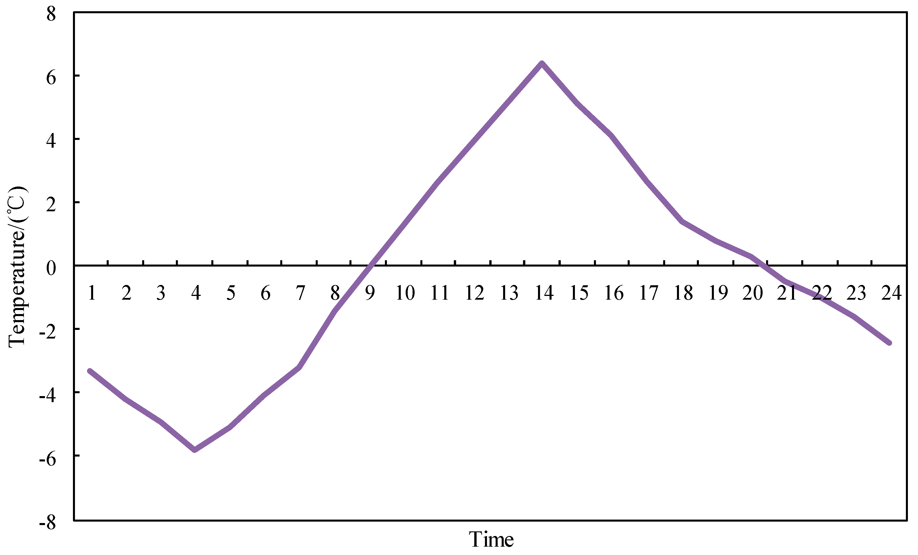
This paper assumes that all four types of consumers are involved in the FDR project of electric load. The dispatching results are analyzed when the level of consumer’s participation in the FDR project (the proportion of shiftable load occupying total electric load) is 5%, 10% and 20%, respectively. Four types of users are involved in the FDR project of thermal load. Assuming that thermal load in the case is heating load, the outdoor temperature curve is shown in Figure A1. The temperature comfort ranges of heating load are constant 20 °C, 20 ± 1 °C, and 20 ± 2 °C, respectively.

5.2. Simulation Results and Analysis

5.2.1. Benefit Analysis for FDR of Electric and Thermal Load

As illustrated in

Table 5. Costs of the system operation with FDR of electric and thermal load (Unit: ¥).

FDR-Temperature Range of the Heating Load	FDR-Ratio of the Shiftable Load
	0%	5%	10%	20%
Constant 20 °C	239,060	237,280	235,230	231,550
[19,21] °C	237,390	235,610	223,530	229,780
[18,22] °C	235,740	223,960	221,880	228,100

, with the increase of consumer’s participation in FDR, the total cost of the system operation will be reduced. The influence of the increase of shiftable load ratios and the temperature comfort range of heating load is significant. The total cost of 20% shiftable load ratio and 20 ± 2 °C heating temperature comfort range is reduced by 4.58% compared with that of the scenario without considering FDR (The analysis below is based on this scenario without the special explanation). The total electric power consumption remains unchanged after the implementation of the FDR of electric load, but due to the load transfer, the valley period and the flat period with lower electricity prices or the period with more abundant electricity can be used to meet load demand, which reduces the cost of the electric load supply. After the implementation of the FDR of thermal load, the cost of thermal load supply is reduced by keeping the indoor temperature of each district within the comfort constraints, and timely regulating the thermal load supply.

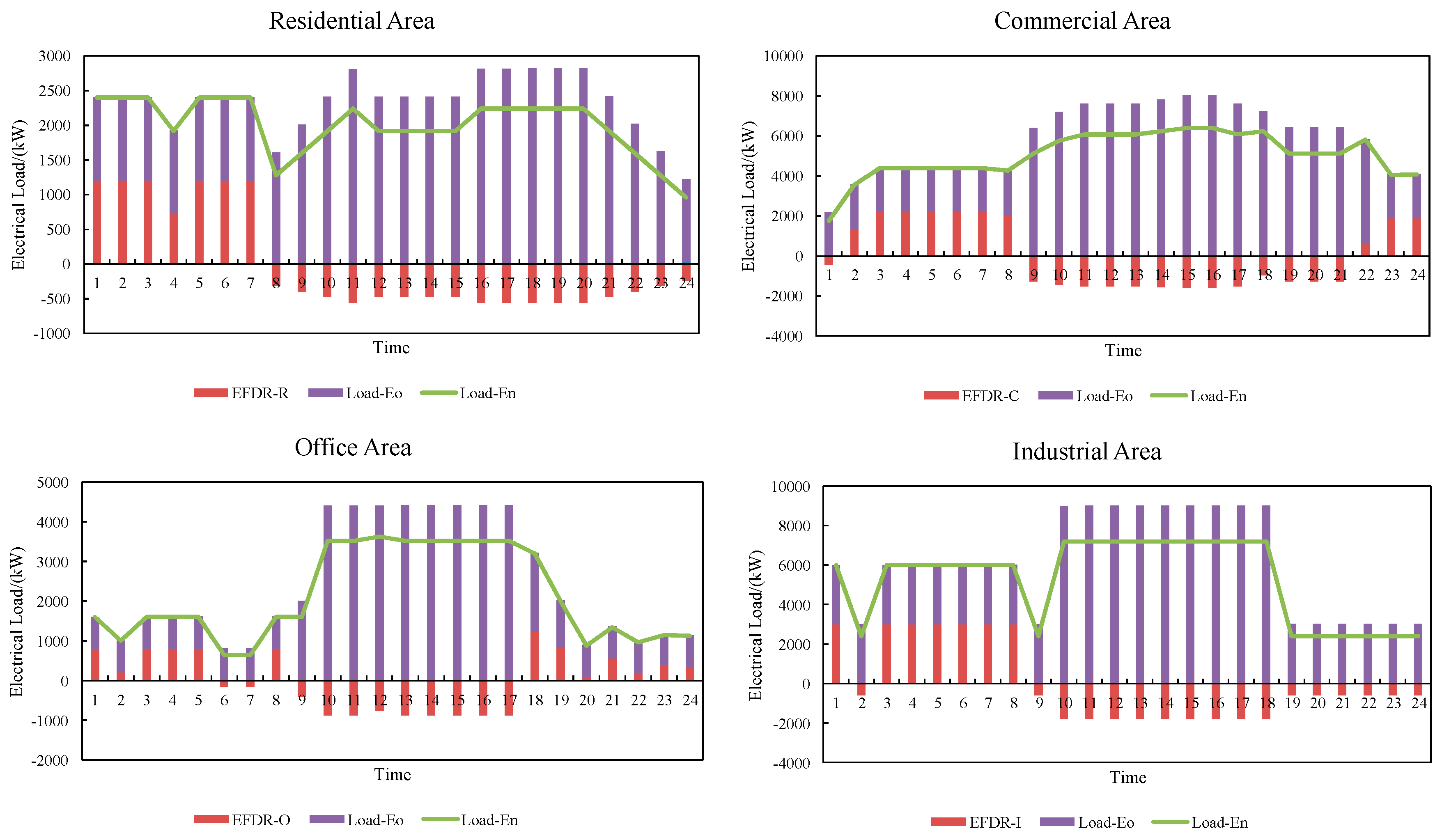
Figure 6 shows the load transfer of residential and industrial districts. EFDR represents the transfer amount of electric load. Load-Eo represents the original electric load. Load-En represents the optimized electric load. The implementation of FDR of electric load effectively reduces the peak-valley difference of electric load in each district. Load in the period of high electricity price is transferred to the periods of high wind power generation or low electricity price, which plays the role of reducing peak and filling valley.

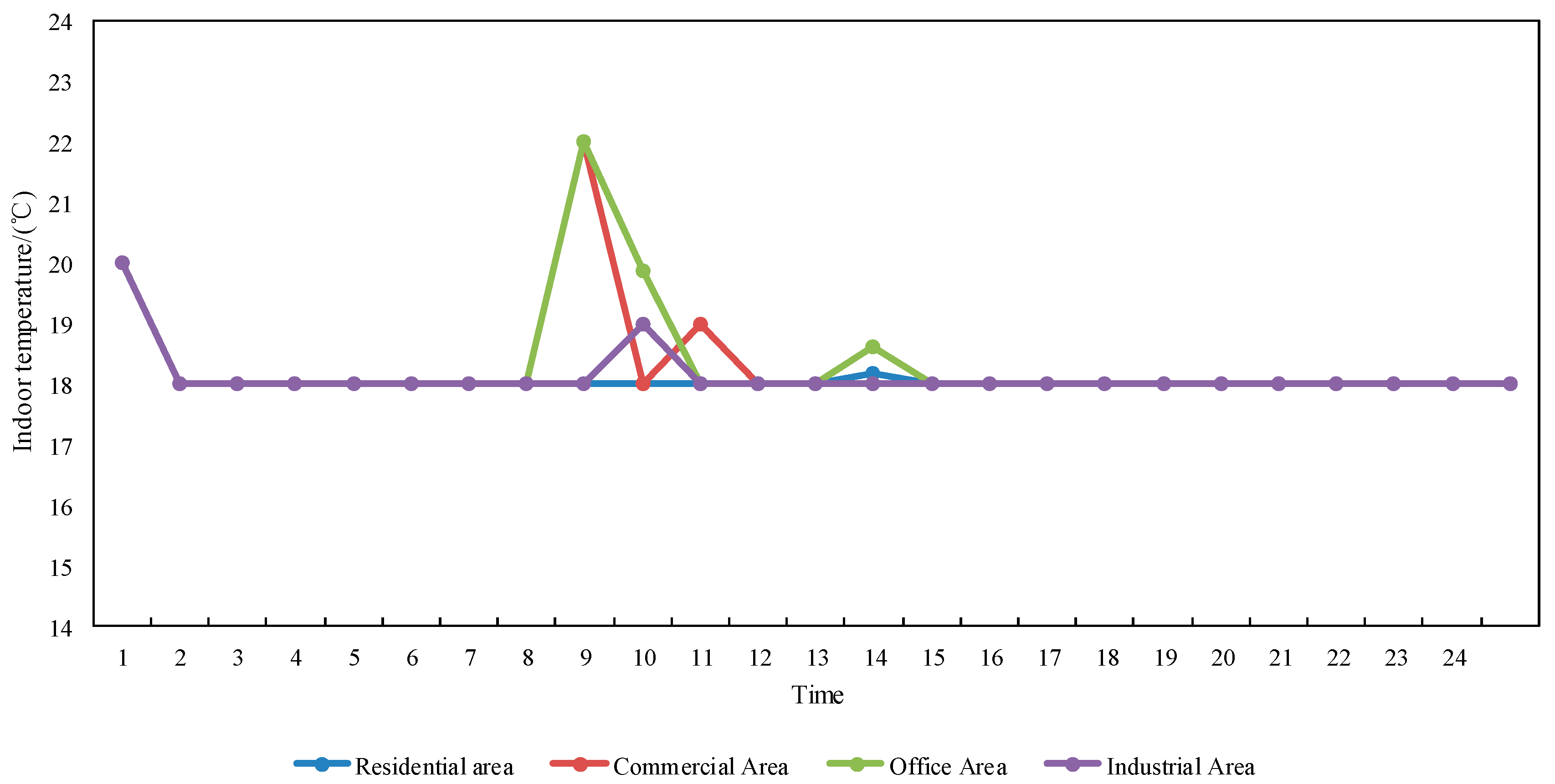
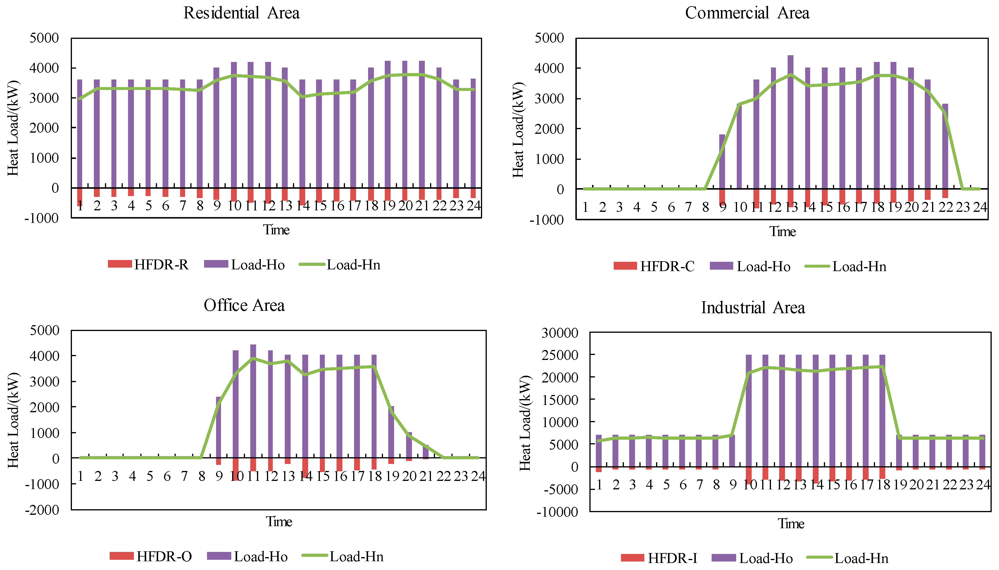
Figure 7 shows the indoor temperature in each district. It can be seen that the indoor temperature after optimization is satisfied with the constraints of consumer’s comfort, and the indoor temperature is maintained in the range of 20 ± 2 °C. Figure 8 shows the situation of thermal load regulation. HFDR represents the heating load regulation. Load-Ho represents the original heating load. Load-Hn represents the optimized heating load. The implementation of FDR of thermal load reduces the heating load supply and directly reduces the total operating cost under the condition of satisfying the consumer’s comfort and providing economic compensation.

5.2.2. Operation Analysis for Multi-District IES

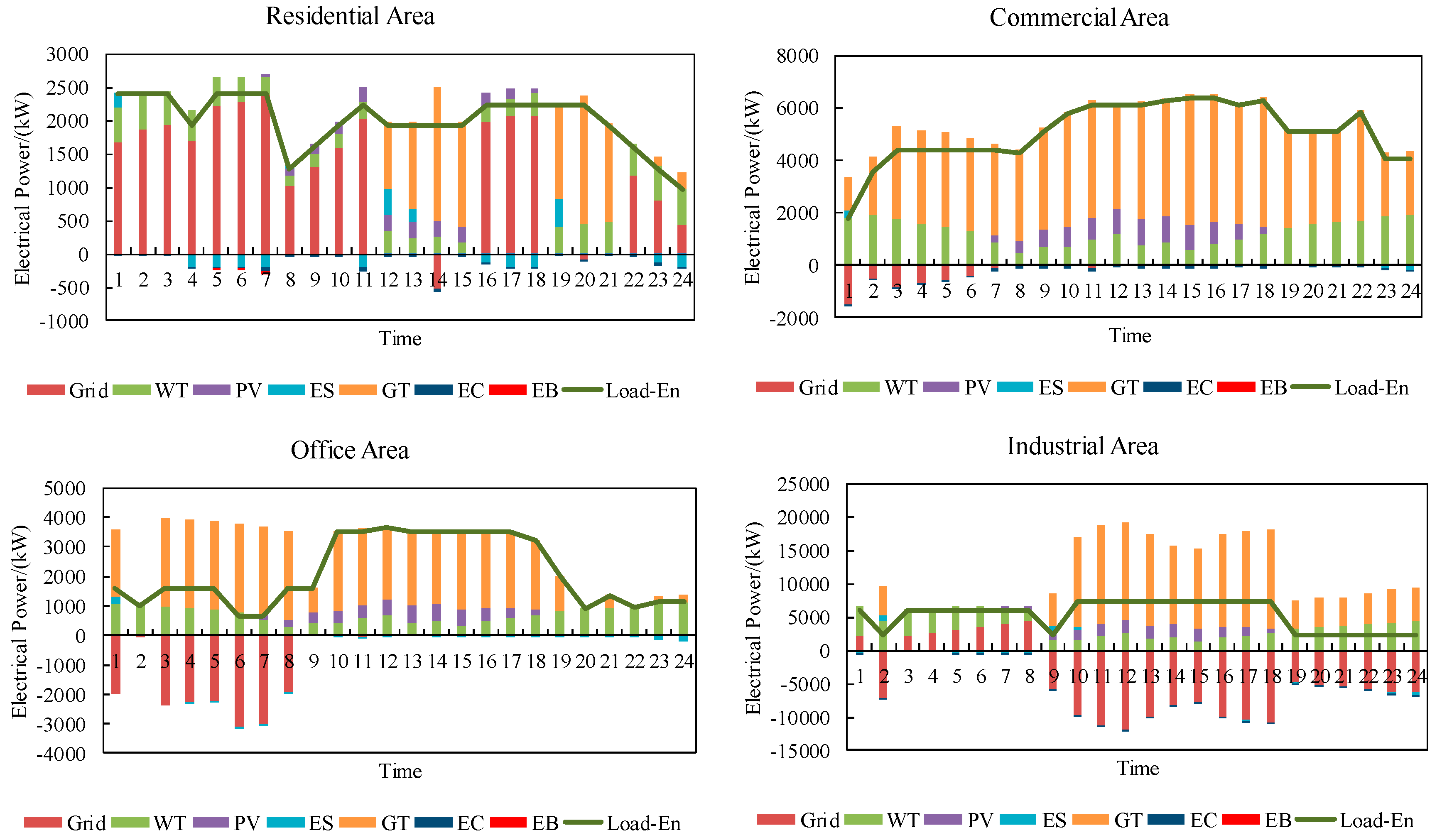
The optimization results of electric power and thermal power in the system are shown in Figure 9 and Figure 10, respectively. The positive power output of the power grid is to indicate that the system purchases electricity from the power grid, while negative power to indicate that the system sells electricity to the power grid. The output of ES is positive to indicate that ES discharges, while negative to indicate that ES charges. The output of HS is positive to indicate that HS releases heat, and negative to indicate that HS stores heat. GT in residential district mainly works at 11:00–15:00 and 18:00–21:00, and the electricity in the remaining periods is mainly purchased from the power grid. The electricity demand in commercial and office districts is mainly met by GT, WT, and PV. There is no need to buy electricity from the grid, and electricity will be sold to the grid when the power is surplus. Power supply in industrial district is mainly met by the power grid, GT, WT, and PV, but GT mainly works at the peak of power grid (8:00–24:00) and sells surplus power to the grid.

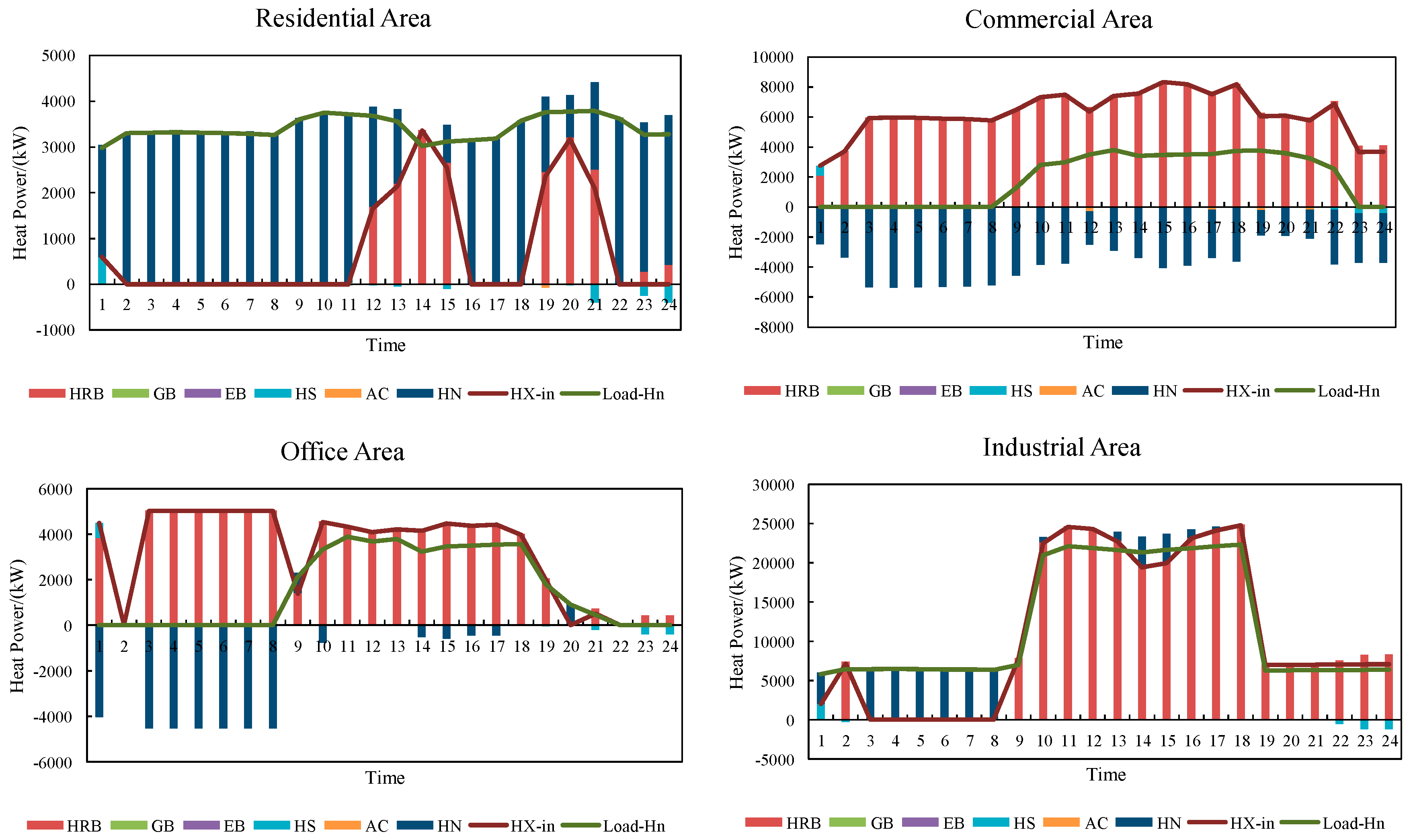
DHN denotes the interactive heating power between each district of multi-district IES and the heating network. The positive value denotes the heating power obtained from the heating network, and negative denotes the heating power injected into the heating network. As can be seen from Figure 10, most of the heating energy supply in residential district is obtained by the heating network, and GT mainly produces heating energy at 11:00–15:00 and 18:00–21:00. Industrial district also obtains heating energy from the heating network, but most of its heating energy is generated by its GT. Obviously, the load of residential and industrial districts is relatively high, so more heating energy is obtained from the heating network. The load of commercial and office areas is relatively low. During the operation, the surplus heat energy of them is transferred to residential and industrial districts through the heating network. It can be seen that the district heating network achieves the coordinated distribution of heating energy among different districts, further improves the efficiency of heating energy utilization, and reduces the operating cost of the system.

5.2.3. Analysis of Heating Network Condition and Benefit

(1) Operation conditions of the heating network

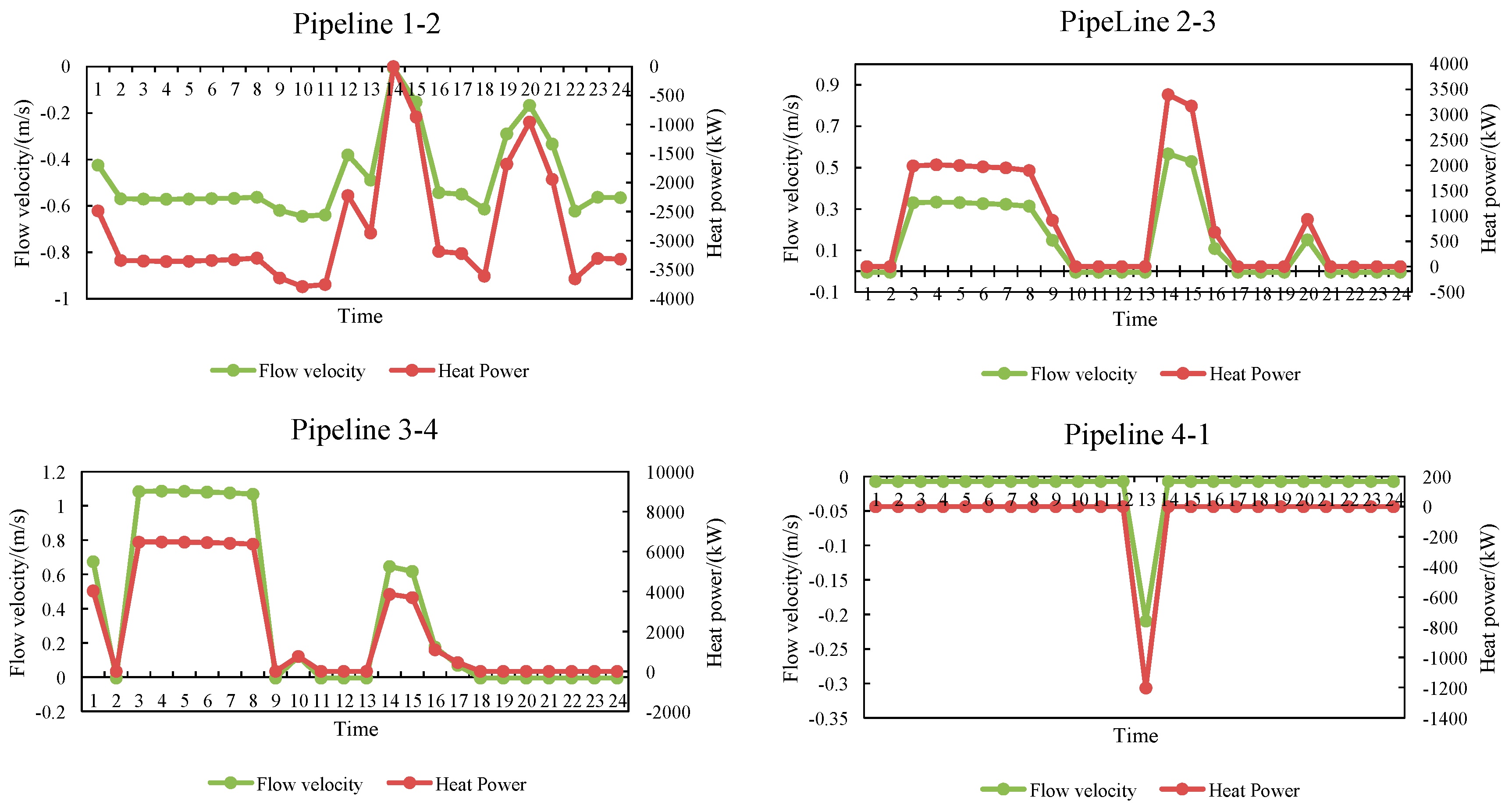
The velocity and power of heating medium in the heating network are shown in Figure 11. The value of clockwise flow of the heating medium is positive, and that of counter-clockwise flow is negative. According to Figure 11, it can be seen that the curve trend of velocity of heating medium and heating power is the same, which satisfies the actual operation constraints of the heating network. It can be concluded that: IES-1 mainly obtains thermal energy from IES-2, and only at 12:00–13:00, IES-4 provides thermal energy for IES-1. IES-2 mainly acts as a thermal energy transporter, conveying thermal energy outward through pipelines 1-2 and 2-3. IES-3 mainly acts as a thermal energy transporter, conveying heat energy to IES-4 through pipelines 3-4. IES-4 only obtains thermal energy from IES-3 during the whole operation cycle. These conclusions are consistent with Figure 10.

(2) Benefit analysis of the heating network

This paper makes a comparative analysis of the heating network operating benefits, ES and HS. The results are shown in

Table 6. Comparison of operating benefits among the district heating network, ES, and HS (Unit: ¥).

Case	DHN	ES	HS	Ce,b	Ce,s	Cgas	CHN	ChFDR	CMD-IES
1	√	√	√	18,949	97,660	295,650	395	10,770	228,100
2	√	√	×	19,114	96,497	293,290	404	10,778	227,080
3	√	×	√	17,539	96,380	295,330	411	10,798	227,700
4	√	×	×	17,690	95,235	293,060	419	10,752	226,680
5	×	√	√	54,185	99,147	285,690	0	8625	249,350
6	×	×	√	51,899	99,392	287,550	0	8626	248,680
7	×	√	×	56,307	97,574	281,390	0	8625	248,750
8	×	×	×	55,418	97,355	281,390	0	8625	248,080

. Comparing case 1 with case 5, it can be seen that when the system does not contain the heating network, the cost of the purchasing electricity increases significantly. The compensation cost of FDR for thermal load and the cost of natural gas decreases slightly. The daily operation cost of multi-district IES with the heating network decreases by 8.52% compared with that without the heating network. The existence of the heating network will directly affect the cost of purchasing electricity and the cost of FDR compensation for thermal load. The reason is that the heating network provides a direct energy coupling exchange channel for districts in the IES, redistributes the heat-to-electric ratios among districts, and reduces the total cost of the IES operation. In addition, comparing case 1 with cases 2~4, and case 5 with cases 6~8, it can be found that the total operating cost increases when the IES is equipped with ES and HS. Considering that the role of the heating network has met the optimal operating requirements of the system in the case, the addition of energy storage devices is needless. Their self-consumption rates lead to the reaction of the increasing cost after joining. The total operating cost of case 1 (without considering the self-consumption rates) is 226,190 ¥, which is 490 ¥ lower than that of case 4. The total operating cost of case 5 (without considering the self-consumption rates) is 247,140 ¥, which is 940 ¥ lower than that of case 8. This further verifies that the role of energy storage devices in this example is not obvious, and its own electric and thermal loss increases the total operating cost. Therefore, the number and capacities of energy storage devices must be reasonably set up in the actual planning process of multi-district IES with heating networks to ensure the operation economy.

5.2.4. Analysis in Economy

(1) Sensitivity analysis of the real-time compensation price of thermal load

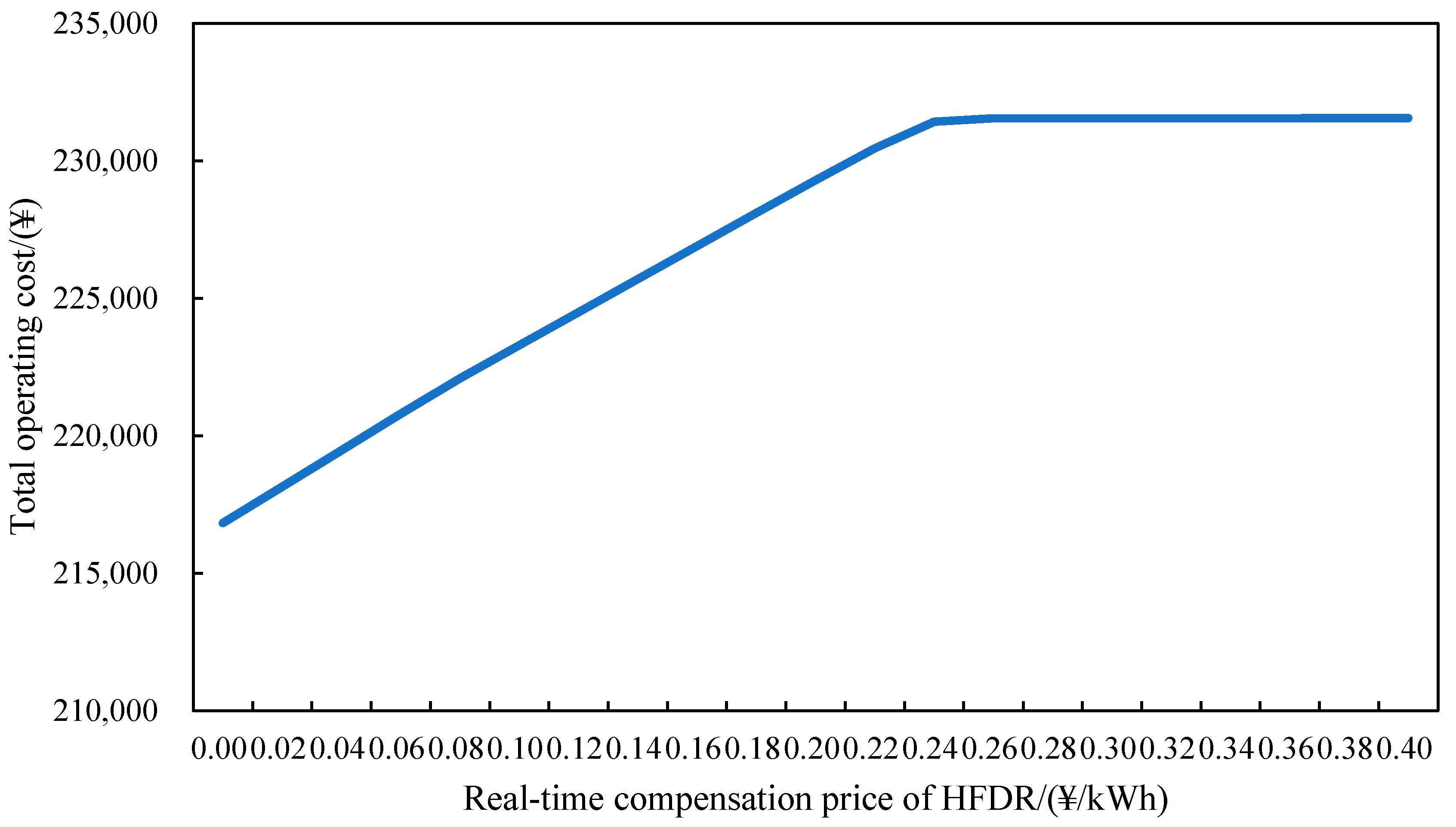
In this paper, the sensitivity analysis of the real-time compensation price for thermal load is carried out. The result is shown in Figure 12. Without considering the real-time compensation of FDR for thermal load, the total operating cost of the system can be reduced to 216,825 ¥, which is 6.36% lower than that of $b_{\mathrm{h}}^{\mathrm{FDR}}>0.26\yen /\left(\mathrm{kWh}\right)$. With the increase of the real-time compensation price, the total operating cost is also increasing, which is approximately linear. When $b_{\mathrm{h}}^{\mathrm{FDR}}>0.26\yen /\left(\mathrm{kWh}\right)$, the cost is approximately maintained at 231,547 ¥. According to the calculation example, it is found that thermal load no longer participates in FDR. This is because the compensation price is close to the calorific value price of natural gas. Considering the loss of thermal power flowing in the system, the system will not excavate the benefit of HDR for thermal load. The system directly meets the heating load supply.

(2) Sensitivity analysis of the calorific value price of natural gas

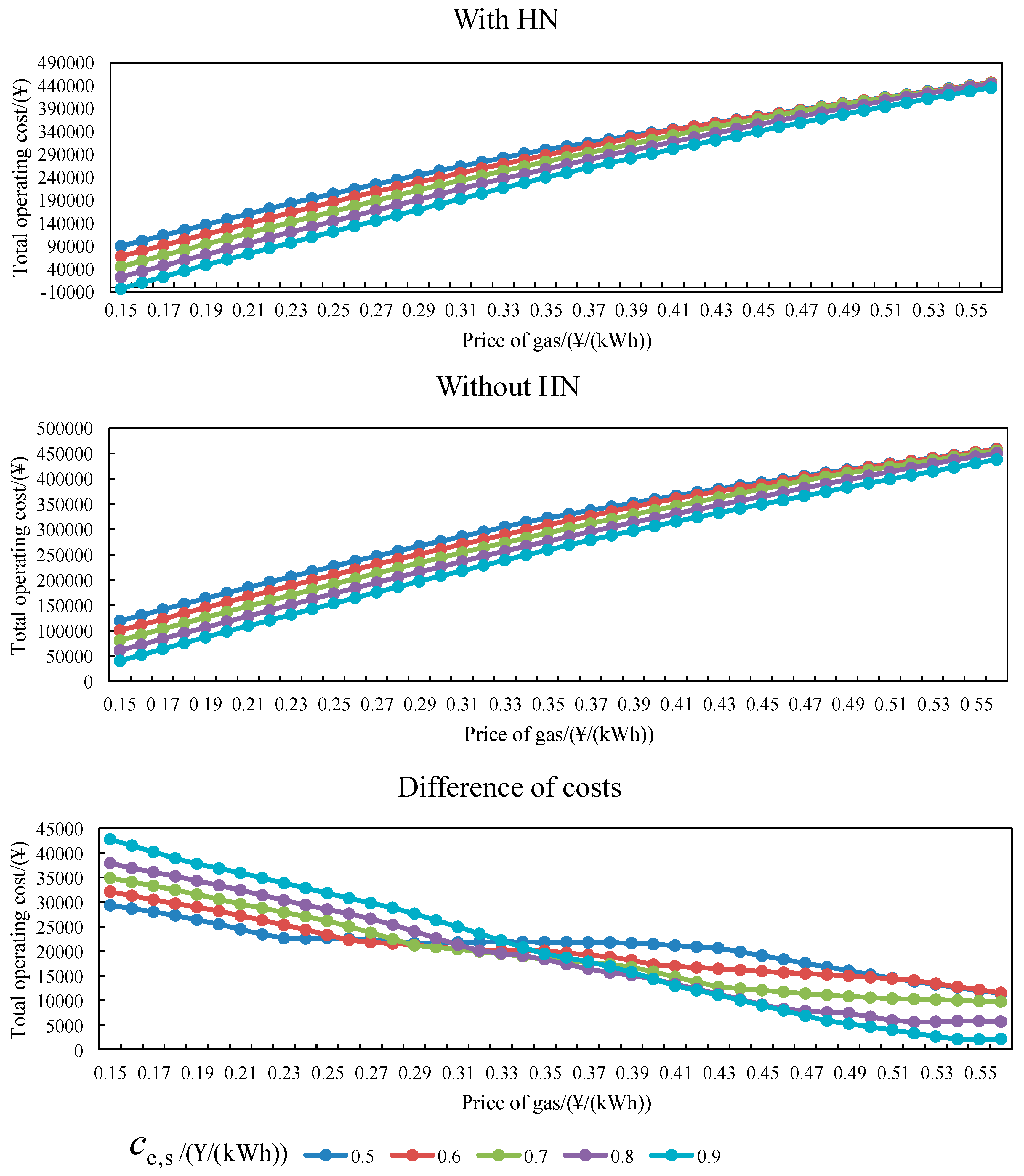
Figure 13 shows the relationships among the operating cost, the difference of operating cost (the difference between the total operating cost of the system without heating network and the total operating cost of the system with heating network) and the price of natural gas under different electricity prices. With or without the heating network, the total operating cost increases with the calorific value price of natural gas. The difference of the operating cost shows a downward trend. The total operating cost of the system taking different electricity selling prices also shows a similar trend with the increase of the calorific value price of natural gas. It can be seen that when $c_{\mathrm{gas}}$ is greater than a certain critical value, the operating conditions with and without heating network tend to be consistent.

Table 7. Relation between the total operating cost and the price of natural gas with the heating network when c_e,s = 0.7 ¥/kWh.

Cgas/(¥/kWh)	Ce,b/(¥)	Ce,s/(¥)	Cgas/(¥)	CHN/(¥)	ChFDR/(¥)	CMD-IES/(¥)
0.15	18,462	155,510	182,400	580	0	45,929
0.25	18,959	147,570	294,150	509	0	166,050
0.35	26,063	101,270	338,720	395	10,823	274,730
0.45	47,152	783,01	387,500	519	10,831	367,700
0.55	77,609	6950	356,310	684	11,746	439,400

and

Table 8. Relation between the total operating cost and the price of natural gas without the heating network when C_e,s = 0.7 ¥/kWh.

Cgas/(¥/kWh)	Ce,b/(¥)	Ce,s/(¥)	Cgas/(¥)	CHN/(¥)	ChFDR/(¥)	CMD-IES/(¥)
0.15	40,201	135,960	170,170	0	6427	80,834
0.25	44,804	130,120	271,480	0	6055	192,220
0.35	69,089	112,270	325,450	0	10,780	293,050
0.45	99,891	102,290	371,370	0	10,805	379,770
0.55	123,260	34,882	349,160	0	11,720	449,260

give the operating costs of different calorific value prices of natural gas with and without heating networks, respectively when $c_{\mathrm{e},\mathrm{s}}=0.7$ ¥/kWh. It can be seen that when $c_{\mathrm{gas}}$ is low, the coupling of multi-district load (mainly heating load) makes its economic benefit more remarkable. Essentially, by transferring heating load, the heat-to-electric ratios of load in some districts is increased, while the heat-to-electric ratios of load in other districts is reduced. GT in the district with the high heat-to-electric ratio of load can bring greater economic benefit. With the increase of $c_{\mathrm{gas}}$, the electricity purchased from the power grid shows an upward trend, and the electricity sold to the power grid is decreasing. The system tends to consume more electricity to meet the load demand. GT tends to produce less heat abandonment and make full use of its heat energy. In addition, the system is more inclined to meet thermal load demand directly when $c_{\mathrm{gas}}$ is lower. When $c_{\mathrm{gas}}$ increase to a critical value, the system will excavate FDR resources of thermal load.

(3) Sensitivity analysis of the heat-to-electric ratio of GT

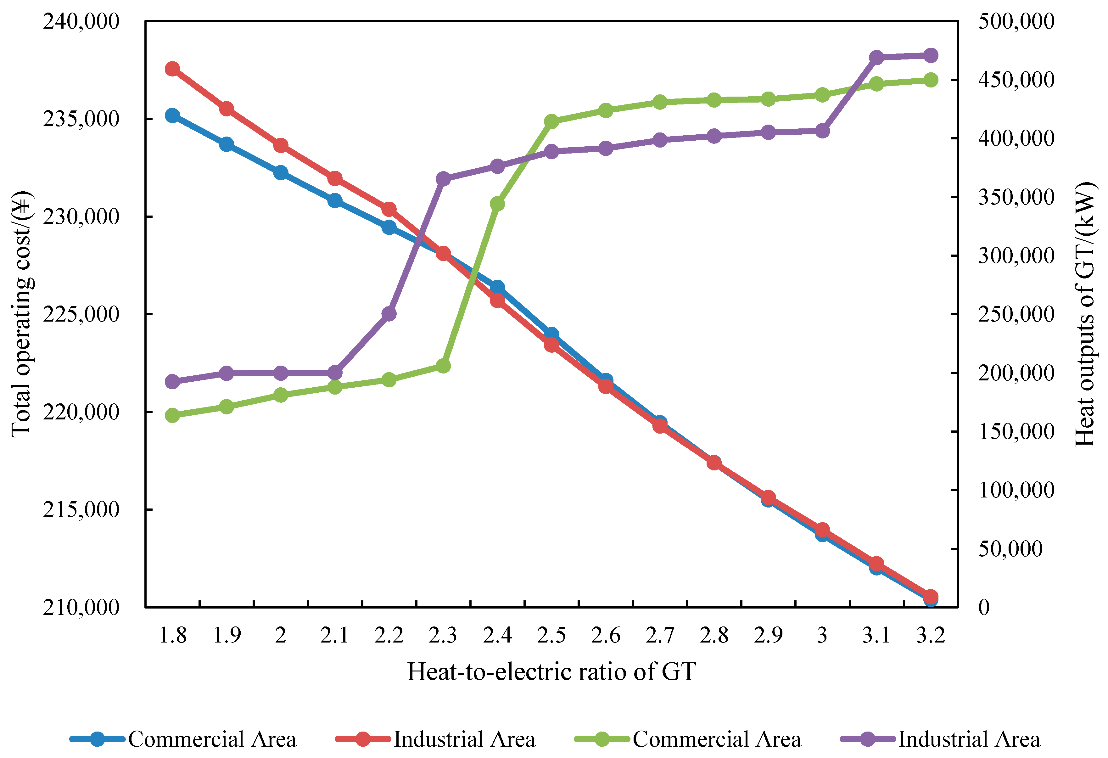
The influence of the heat-to-electric ratio of GT on the operation economy of IES-2 (commercial consumer) and IES-4 (industrial consumer) with high heating load is analyzed. By changing the heat-to-electric ratio of GT in these two districts, the relationship curve between the total operating cost and the heat-to-electric ratio can be obtained, as shown in Figure 14. For IES-2 with the lower heat-to-electric ratio of load and IES-4 with the higher heat-to-electric ratio of load, increasing the heat-to-electric ratio of GT can reduce the total operating cost. This is due to the high proportion of heating load in the example. After the heat-to-electric ratio of GT is increased, only less gas consumption is needed to meet the heating load demand, which directly reduces the gas consumption. According to Table 5, the gas cost occupies the main part of the total cost. Obviously, when IES operates independently in a single district, the change of the heat-to-electric ratio of GT has little effect on the electric and thermal power scheduling in the system, but for multi-district IES with the heating network, the change of the heat-to-electric ratio of GT in any district will cause the redistribution of heating load, and the district with higher heat-to-electric ratio will produce more thermal power.

6. Conclusions

Based on the comprehensive consideration of FDR of electric and thermal load, the IES energy coupling structure and operation characteristics of heating networks, a multi-district IES operation optimization model considering FDR of electric and thermal load is proposed. Through the case simulation and theoretical study, the following conclusions can be drawn:

(1) The FDR control strategy of electric and thermal loads is introduced. On the premise of meeting the demand of electric and thermal loads in different IES districts, the elasticity and flexibility of supply side and demand side are increased by transferring electric load, reducing real-time thermal load. The peak-valley difference of electric and thermal load, and the total operating cost of the system are effectively reduced.

(2) The optimal operation model of multi-district IES with the DHN is proposed. On the one hand, it can realize the optimal operation condition of the equipment in each district and achieve the optimal work coordination. On the other hand, the load characteristics of different districts can be coupled through the DHN. The complementary characteristics can be used to optimize the energy flow and improve the operation economy.

(3) The application of the DHN in multi-district IES with large electric and thermal load and uneven distribution of heat-to-electric ratios among sub-districts is more significant. By connecting CCHP systems in different districts through the DHN, the coordinated distribution of energy among sub-districts can be realized. The utilization efficiency of thermal energy can also be improved. The role of the DHN is essentially to transfer heating load to redistribute the heat-to-electric ratios to achieve the optimal operation of the system. Based on the example in this paper, the interconnection of DHN also plays the role of substituting ES and HS in each sub-district, which can reduce the investment cost of energy storage devices in the planning and construction.