Estimation of Oil Recovery Factor for Water Drive Sandy Reservoirs through Applications of Artificial Intelligence


Abstract
:1. Introduction
2. Background of Empirical Correlations Used for Recovery Factor Estimation
3. Applications of Artificial Intelligence in the Petroleum Industry
4. Materials and Methods
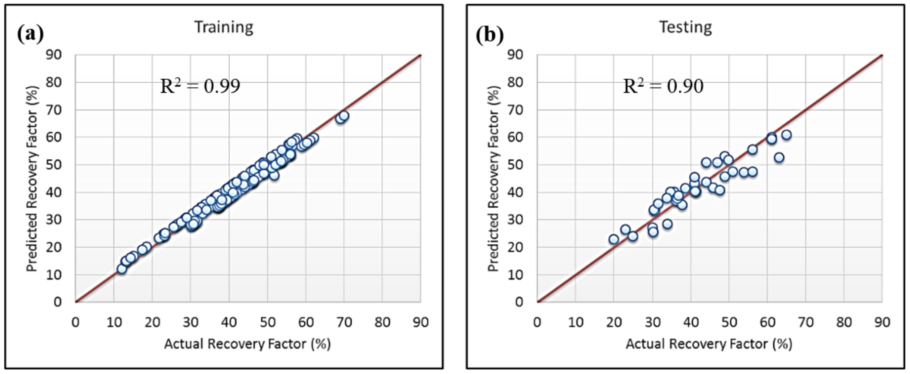
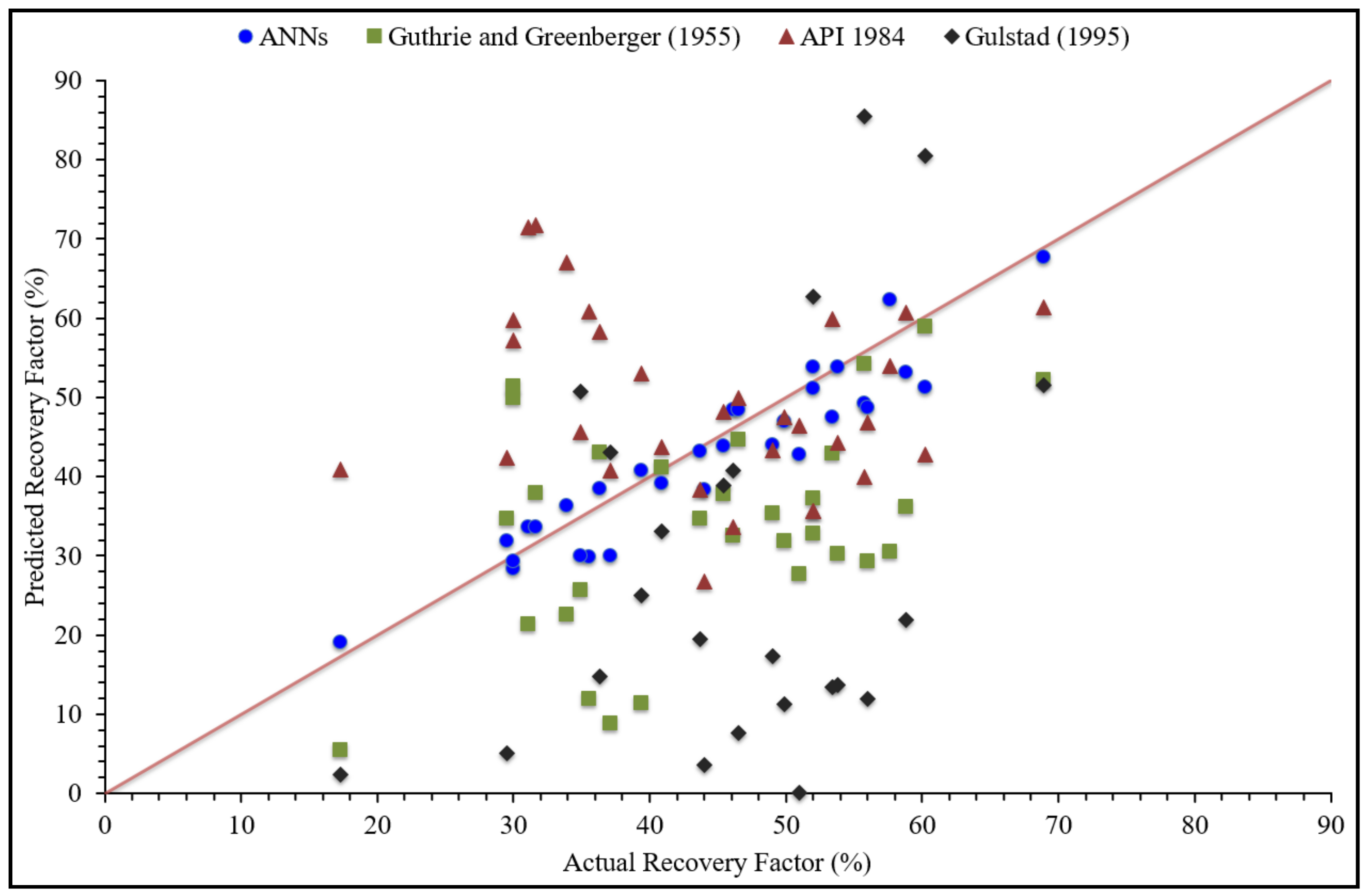
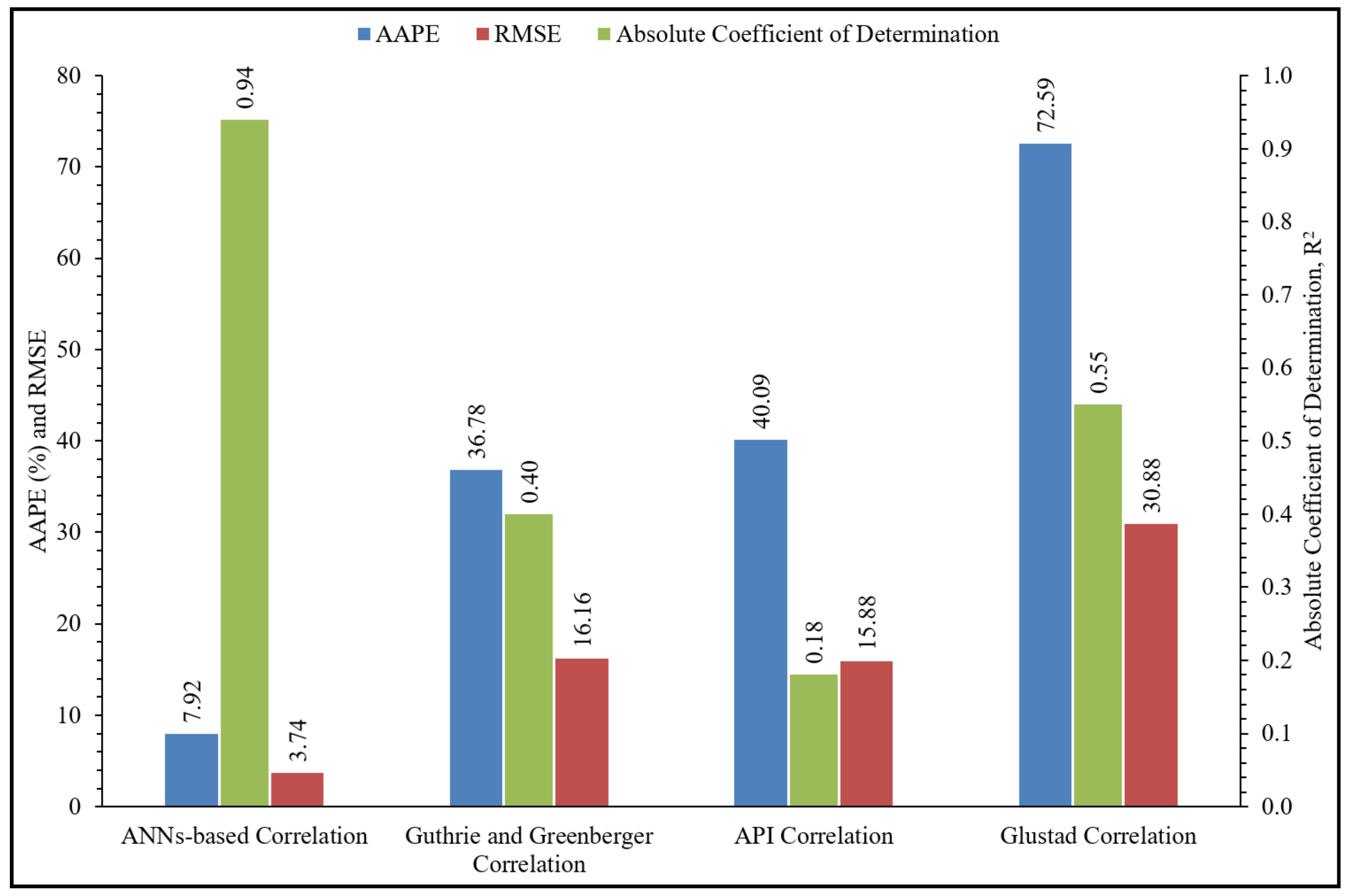
5. Results and Discussion
6. Conclusions
Author Contributions
Funding
Conflicts of Interest
Nomenclature
| AAPE | Absolute Average Percentage Error |
| AI | Artificial Intelligence |
| ANFIS-SC | Adaptive Neuro-Fuzzy Inference System with Subtractive Clustering |
| ANNs | Artificial Neural Networks |
| API | American Petroleum Institute |
| STOIIP | Stock-Tank Oil Initially in Place |
| R2 | Coefficient of Determination |
| RF | Recovery Factor |
| RFa | Actual Correlation Factor |
| RFm | Estimated Correlation Factor |
| RNNs | Radial Basis Neural Networks |
| RMSE | Root Mean Square Error |
| SD | Standard Deviation |
| SVM | Support Vector Machines |
Appendix A
References
- Noureldien, D.M.; El-Banbi, A.H. Using Artificial Intelligence in Estimating Oil Recovery Factor. In Proceedings of the SPE North Africa Technology Conference and Exhibition, Cairo, Egypt, 14–16 September 2015. [Google Scholar] [CrossRef]
- Ahmed, A.A.; Elkatatny, S.; Abdulraheem, A.; Mahmoud, M. Application of Artificial Intelligence Techniques in Estimating Oil Recovery Factor for Water Derive Sandy Reservoirs. In Proceedings of the SPE Kuwait Oil & Gas Show and Conference, Kuwait City, Kuwait, 15–18 October 2017. [Google Scholar] [CrossRef]
- Craft, B.C.; Hawkins, M. Applied Petroleum Reservoir Engineering, 3rd ed.; Pearson Education, Inc.: London, UK, 2015. [Google Scholar]
- Ahmed, T. Reservoir Engineering Handbook, 4th ed.; Gulf Professional Publishing: Houston, TX, USA, 2010. [Google Scholar]
- Lee, J.; Wattenbarger, R.A. Gas Reservoir Engineering; Society of Petroleum Engineers: Houston, TX, USA, 1996. [Google Scholar]
- Dake, L.P. Fundamentals of Reservoir Engineering. In Chapter 4, Reservoir Engineering; Elsevier Science: Amsterdam, The Netherlands, 1983. [Google Scholar]
- Agarwal, R.G.; Gardner, D.C.; Kleinsteiber, S.W.; Fussell, D.D. Analyzing Well Production Data Using Combined Type Curve and Decline Curve Analysis Concepts. In Proceedings of the SPE Annual Technical Conference and Exhibition, New Orleans, LA, USA, 27–30 September 1998. [Google Scholar] [CrossRef]
- Guthrie, R.K.; Greenberger, M.H. The Use of Multiple-correlation Analyses for Interpreting Petroleum-engineering Data. In Proceedings of the Drilling and Production Practice; American Petroleum Institute: Washington, DC, USA, 1955; pp. 130–137. [Google Scholar]
- Gulstad, R.L. The Determination of Hydrocarbon Reservoir Recovery Factors by Using Modern Multiple Linear Regression Techniques. Master’s Thesis, Texas A&M University, College Station, TX, USA, 1995. [Google Scholar]
- Craze, R.C.; Buckley, S.E. A factual analysis of the effect of well spacing on oil recovery. In Proceedings of the Drilling and Production Practice; American Petroleum Institute: Washington, DC, USA, 1945; pp. 144–159. [Google Scholar]
- Muskat, M.; Taylor, M.O. Effect of Reservoir Fluid and Rock Characteristics on Production Histories of Gas-Drive Reservoirs. Trans. AIME 1946, 165, 78–93. [Google Scholar] [CrossRef]
- Arps, J.J.; Roberts, T.G. The effect of the relative permeability ratio, the oil gravity, and the solution gas-oil ratio on the primary recovery from a depletion type reservoir. Pet. Trans. 1955, 204, 120–127. [Google Scholar]
- Mahmoud, A.A.A.; Elkatatny, S.; Mahmoud, M.; Abouelresh, M.; Abdulraheem, A.; Ali, A. Determination of the total organic carbon (TOC) based on conventional well logs using artificial neural network. Int. J. Coal Geol. 2017, 179, 72–80. [Google Scholar] [CrossRef]
- Mahmoud, A.A.; Elkatatny, S.; Abdulraheem, A.; Mahmoud, M.; Ibrahim, M.O.; Ali, A. New Technique to Determine the Total Organic Carbon Based on Well Logs Using Artificial Neural Network (White Box). In Proceedings of the SPE Kingdom Saudi Arabia Annual Technical Symposium and Exhibition, Dammam, Saudi Arab, 24–27 April 2017. [Google Scholar] [CrossRef]
- Elkatatny, S.A.; Mahmoud, M.A. Development of a New Correlation for Bubble Point Pressure in Oil Reservoirs Using Artificial Intelligent Technique. Arab. J. Sci. Eng. 2018, 43, 2491–2500. [Google Scholar] [CrossRef]
- Elkatatny, S.M. Real Time Prediction of Rheological Parameters of KCl Water-Based Drilling Fluid Using Artificial Neural Networks. Arab. J. Sci. Eng. 2017, 42, 1655–1665. [Google Scholar] [CrossRef]
- Abdelgawad, K.; Elkatatny, S.; Moussa, T.; Mahmoud, M.; Patil, S. Real Time Determination of Rheological Properties of Spud Drilling Fluids Using a Hybrid Artificial Intelligence Technique. J. Energy Resour. Technol. 2018, 141, 032908. [Google Scholar] [CrossRef]
- Elkatatny, S. Application of Artificial Intelligence Techniques to Estimate the Static Poisson’s Ratio Based on Wireline Log Data. ASME. J. Energy Resour. Technol. 2018, 140, 072905. [Google Scholar] [CrossRef]
- Mahmoud, A.A.; Elkatatny, S.; Ali, A. Estimation of Static Young’s Modulus for Sandstone Formation Using Artificial Neural Networks. Energies 2019, 12, 2125. [Google Scholar] [CrossRef]
- Mohaghegh, S.; Arefi, R.; Ameri, S.; Hefner, M.H. A Methodological Approach for Reservoir Heterogeneity Characterization Using Artificial Neural Networks. In Proceedings of the SPE Annual Technical Conference and Exhibition, New Orleans, LA, USA, 25–28 September 1994. [Google Scholar] [CrossRef]
- Barman, I.; Ouenes, A.; Wang, M. Fractured Reservoir Characterization Using Streamline-Based Inverse Modeling and Artificial Intelligence Tools. In Proceedings of the SPE Annual Technical Conference and Exhibition, Dallas, TX, USA, 1–4 October 2000. [Google Scholar] [CrossRef]
- Moussa, T.; Elkatatny, S.; Mahmoud, M.; Abdulraheem, A. Development of New Permeability Formulation From Well Log Data Using Artificial Intelligence Approaches. ASME. J. Energy Resour. Technol. 2018, 140, 072903. [Google Scholar] [CrossRef]
- Al-AbdulJabbar, A.; Elkatatny, S.M.; Mahmoud, M.; Abdelgawad, K.; Abdulaziz, A. A Robust Rate of Penetration Model for Carbonate Formation. J. Energy Resour. Technol. 2018, 141, 042903. [Google Scholar] [CrossRef]
- Al-Shehri, D.A. Oil and Gas Wells: Enhanced Wellbore Casing Integrity Management through Corrosion Rate Prediction Using an Augmented Intelligent Approach. Sustainability 2019, 11, 818. [Google Scholar] [CrossRef]
- Salehi, S.; Hareland, G.; Dehkordi, K.K.; Ganji, M.; Abdollahi, M. Casing collapse risk assessment and depth prediction with a neural network system approach. J. Pet. Sci. Eng. 2009, 69, 156–162. [Google Scholar] [CrossRef]
- Wang, Y.; Salehi, S. Application of real-time field data to optimize drilling hydraulics using neural network approach. J. Energy Resour. Technol. 2015, 137, 062903. [Google Scholar] [CrossRef]
- Ahmed, A.S.; Ahmed, A.A.; Elkatatny, S. Fracture Pressure Prediction Using Radial Basis Function. In Proceedings of the 2019 AADE National Technical Conference and Exhibition, Denver, CO, USA, 9–10 April 2019. [Google Scholar]
- Ahmed, A.S.; Ahmed, A.A.; Elkatatny, S.; Mahmoud, M.; Abdulraheem, A. Prediction of Pore and Fracture Pressures Using Support Vector Machine. In Proceedings of the 2019 International Petroleum Technology Conference, Beijing, China, 26–28 March 2019. [Google Scholar] [CrossRef]
- Adrian, O.; Chukwueke, N. Application of Neural Networks in Developing an Empirical Oil Recovery Factor Equation for Water Drive Niger Delta Reservoirs. In Proceedings of the SPE Nigeria Annual International Conference and Exhibition, Lagos, Nigeria, 5–7 August 2014. [Google Scholar] [CrossRef]
- Onolemhemhen, R.U.; Isehunwa, S.O.; Salufu, S.O. Development of Recovery Factor Model for Water Drive and Depletion Drive Reservoirs in The Niger Delta. In Proceedings of the SPE Nigeria Annual International Conference and Exhibition, Lagos, Nigeria, 2–4 August 2016. [Google Scholar] [CrossRef]

| Group | Parameter | Definition |
|---|---|---|
| Asset Size | Asset area | Asset size in terms of its areal extent and reservoir size. |
| STOIIP | The estimated value of the stock-tank oil initially in place. | |
| Rock Parameters | Net pay thick (h) | The net thickness of oil-saturated sand within the entire reservoir. |
| Porosity (ϕ) | The pore volume relative to the total bulk rock volume of the rock. | |
| Lorenz coeff. | Represents the vertical heterogeneity of the reservoir. | |
| Initial water saturation (Swi) | Value of initial water saturation. | |
| Permeability (k) | Absolute permeability from core analysis. | |
| Fluid Properties | API | API gravity from PVT. |
| Oil viscosity (µo) | Measured or calculated oil viscosity. | |
| Reservoir Energy | Reservoir pressure (p) | Reservoir pressure, referenced at 10,000 ft TVD. |
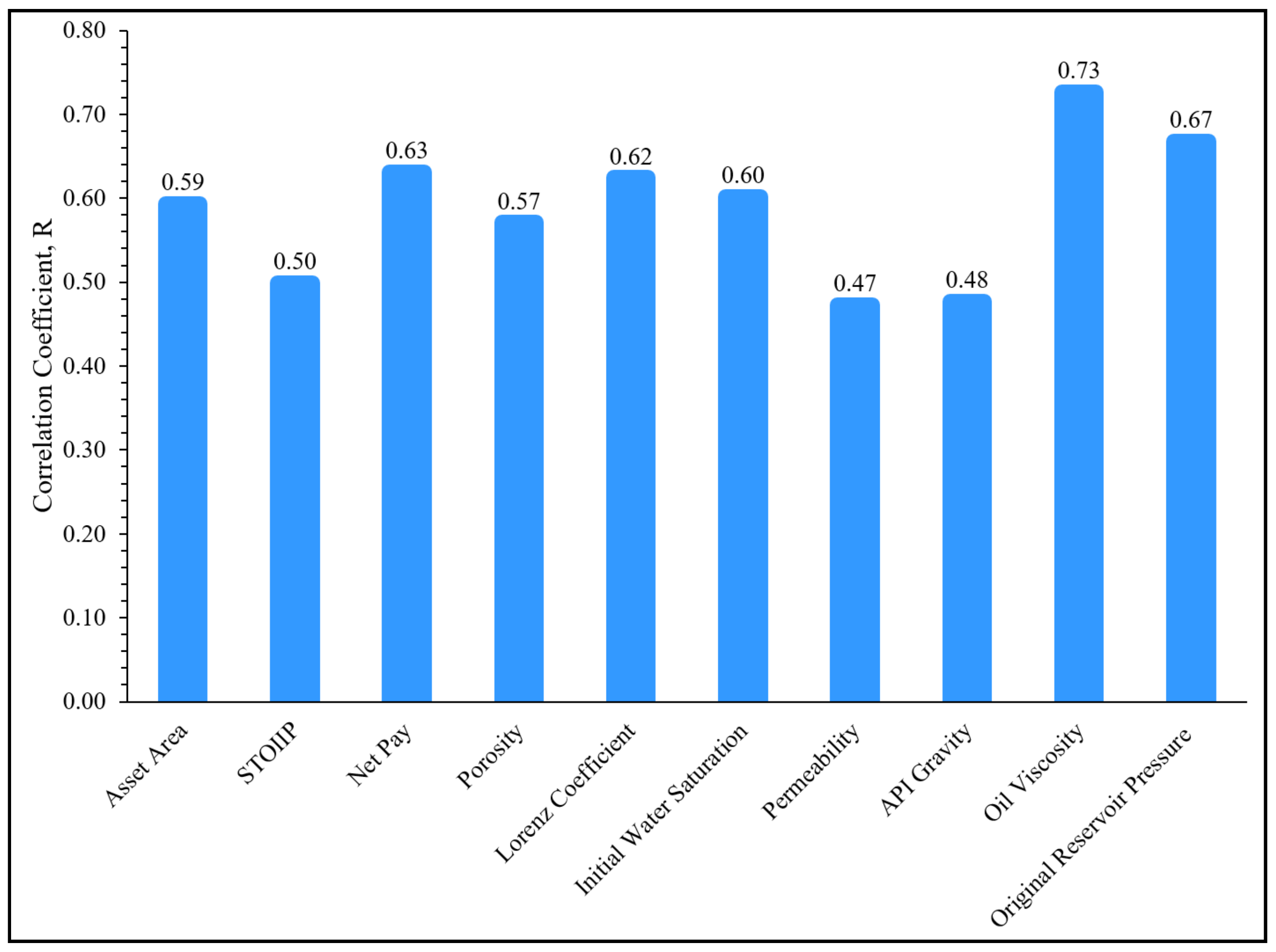
| Input Parameters | Min | Max | Mean | Mode | Range | SD | Coef. of Variation | R2 |
|---|---|---|---|---|---|---|---|---|
| Asset Area (acres) | 446 | 15515 | 4787.5 | 3970 | 15069 | 3094 | 0.646 | 0.352 |
| STOIIP (MMSTB) | 5.00 | 1072.5 | 326.6 | 88 | 1067.5 | 279.1 | 0.854 | 0.249 |
| Net Pay “h” (ft) | 12.9 | 471.45 | 152.9 | 25.7 | 458.6 | 107.8 | 0.705 | 0.399 |
| Porosity (fraction) | 0.12 | 0.32 | 0.234 | 0.23 | 0.2 | 0.04 | 0.173 | 0.326 |
| Lorenz Coefficient (fraction) | 0.15 | 0.77 | 0.442 | 0.24 | 0.62 | 0.118 | 0.268 | −0.390 |
| Swi (fraction) | 0.16 | 0.31 | 0.225 | 0.2 | 0.15 | 0.036 | 0.16 | −0.362 |
| Permeability “k” (md) | 15.0 | 1270 | 450 | 1000 | 1255 | 318.3 | 0.707 | −0.224 |
| API (degree) | 23.0 | 42.20 | 34.50 | 33.0 | 19.2 | 4.446 | 0.129 | 0.228 |
| Oil Viscosity (cp) | 0.16 | 2.59 | 0.874 | 0.6 | 2.43 | 0.548 | 0.627 | 0.528 |
| P “@ 10,000 TVD” (psi) | 1672 | 11470 | 5833.7 | 7000 | 9798 | 2286.4 | 0.392 | 0.446 |
| Input Layer | Output Layer | |||||||||||||
|---|---|---|---|---|---|---|---|---|---|---|---|---|---|---|
| Weights (w1) | Biases (b1) | Weights (w2) | Bias (b2) | |||||||||||
| j = 1 | j = 2 | j = 3 | j = 4 | j = 5 | j = 6 | j = 7 | j = 8 | j = 9 | j = 10 | |||||
| No. of Neurons | i = 1 | 42.15 | 3.82 | 11.27 | −57.13 | −8.42 | −23.59 | −10.34 | 27.35 | 50.09 | 40.05 | −2.06 | 0.07 | −0.49 |
| i = 2 | 40.32 | 4.05 | −7.60 | 8.91 | −5.01 | 9.13 | 11.68 | −14.11 | 16.53 | −21.10 | −1.48 | 0.18 | ||
| i = 3 | −11.13 | 10.73 | −10.68 | −23.31 | −1.18 | 23.48 | 32.23 | 6.22 | −41.03 | −19.40 | −2.27 | 0.29 | ||
| i = 4 | −0.29 | 1.14 | −0.13 | 0.07 | −0.59 | −1.05 | 0.07 | 0.11 | 1.34 | 0.68 | 0.39 | 0.59 | ||
| i = 5 | 2.34 | 0.54 | 0.83 | 0.14 | 0.92 | −4.49 | 0.12 | −9.08 | 4.76 | 0.55 | 2.60 | −0.38 | ||
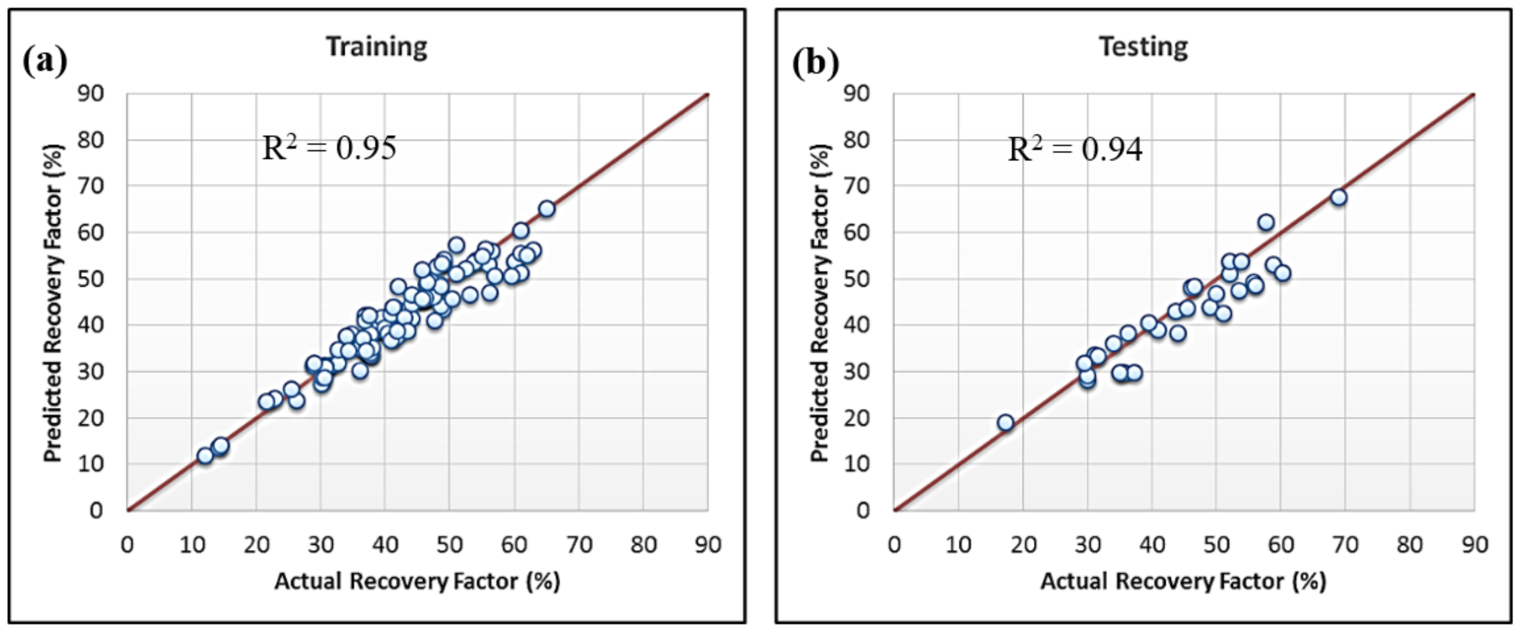
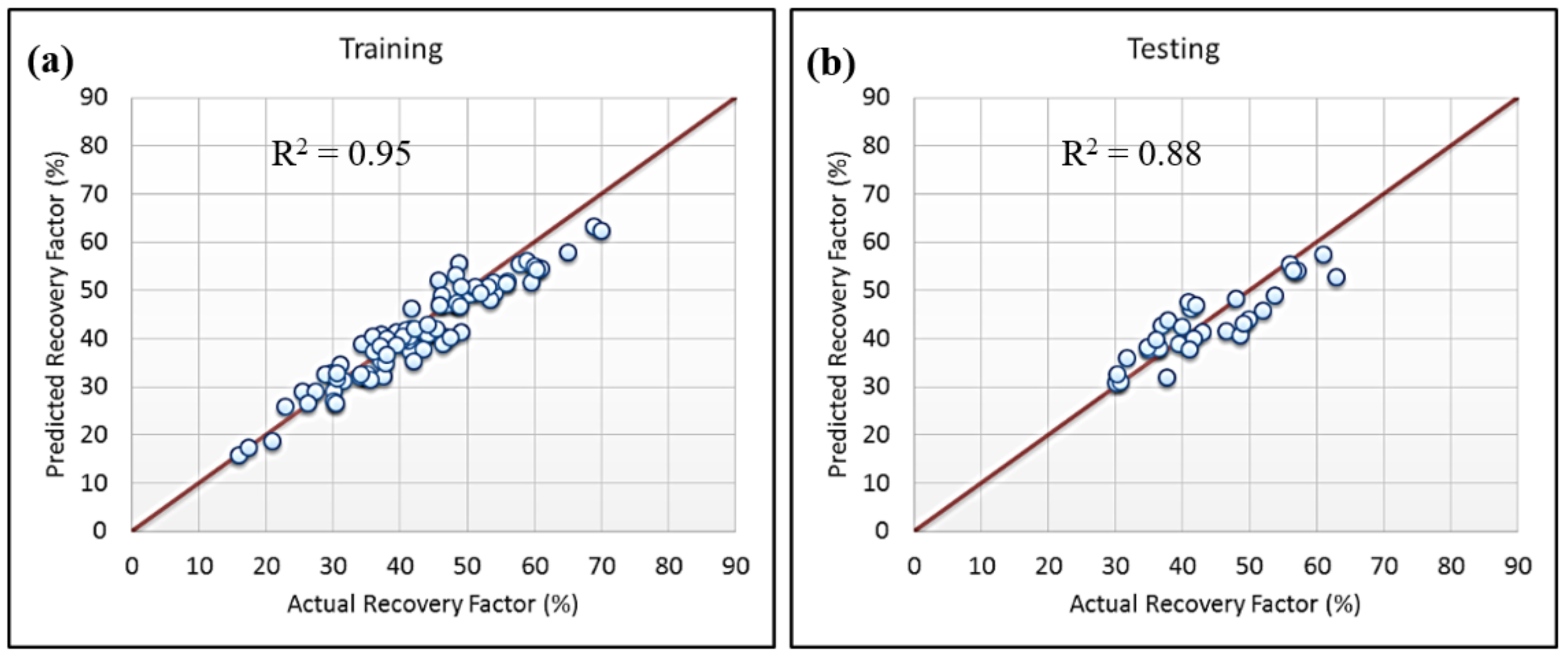
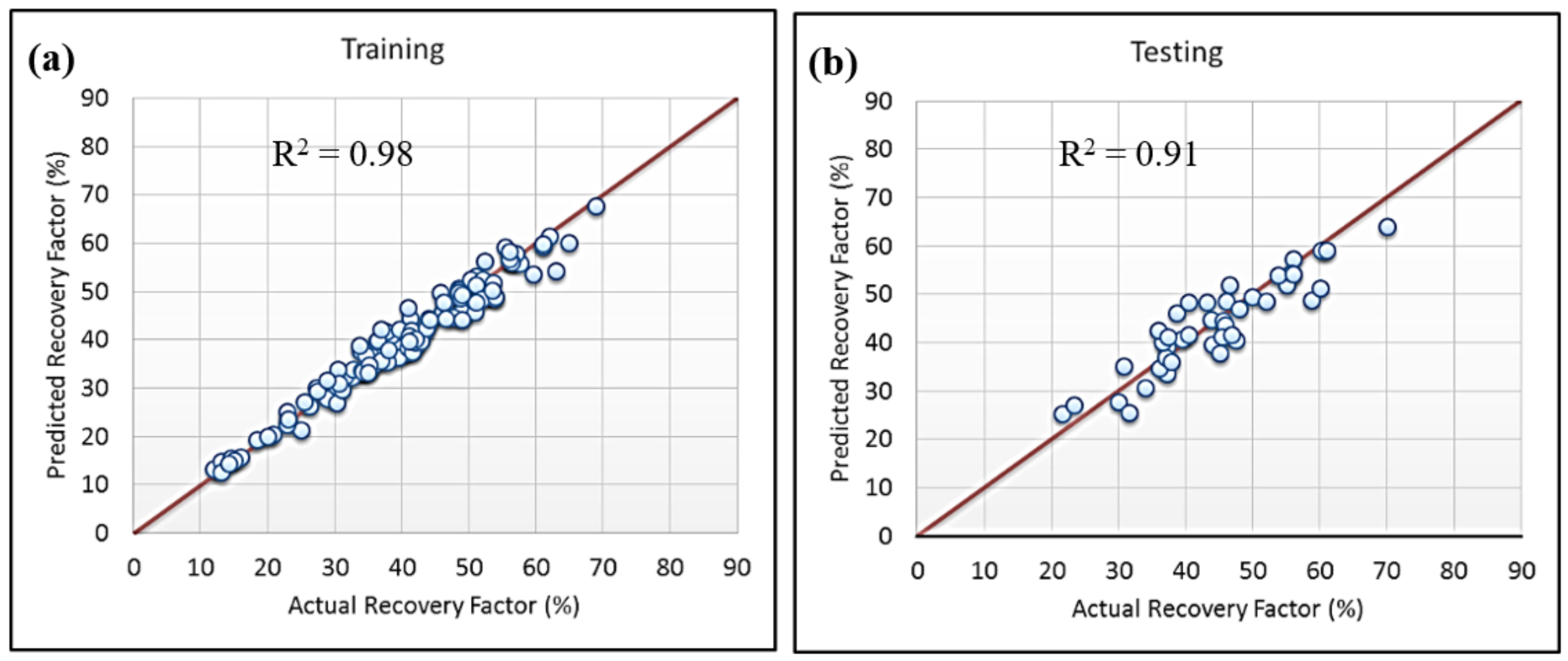
| Training | Testing | |||
|---|---|---|---|---|
| R2 | AAPE (%) | R2 | AAPE (%) | |
| ANNs | 0.95 | 5.80 | 0.94 | 7.92 |
| RNNs | 0.95 | 6.86 | 0.88 | 8.78 |
| ANFIS-SC | 0.98 | 4.83 | 0.91 | 8.53 |
| SVM | 0.99 | 5.11 | 0.90 | 10.44 |
© 2019 by the authors. Licensee MDPI, Basel, Switzerland. This article is an open access article distributed under the terms and conditions of the Creative Commons Attribution (CC BY) license (http://creativecommons.org/licenses/by/4.0/).
Share and Cite
Mahmoud, A.A.; Elkatatny, S.; Chen, W.; Abdulraheem, A. Estimation of Oil Recovery Factor for Water Drive Sandy Reservoirs through Applications of Artificial Intelligence. Energies 2019, 12, 3671. https://doi.org/10.3390/en12193671
Mahmoud AA, Elkatatny S, Chen W, Abdulraheem A. Estimation of Oil Recovery Factor for Water Drive Sandy Reservoirs through Applications of Artificial Intelligence. Energies. 2019; 12(19):3671. https://doi.org/10.3390/en12193671
Chicago/Turabian StyleMahmoud, Ahmed Abdulhamid, Salaheldin Elkatatny, Weiqing Chen, and Abdulazeez Abdulraheem. 2019. "Estimation of Oil Recovery Factor for Water Drive Sandy Reservoirs through Applications of Artificial Intelligence" Energies 12, no. 19: 3671. https://doi.org/10.3390/en12193671
APA StyleMahmoud, A. A., Elkatatny, S., Chen, W., & Abdulraheem, A. (2019). Estimation of Oil Recovery Factor for Water Drive Sandy Reservoirs through Applications of Artificial Intelligence. Energies, 12(19), 3671. https://doi.org/10.3390/en12193671