Wind Farm NWP Data Preprocessing Method Based on t-SNE

Abstract

The operation prediction of wind farms will be accompanied by the need for massive data processing, especially the preprocessing of wind farm meteorological data or numerical weather prediction (NWP). Because NWP data are strongly correlated with wind farm operation, proper processing of NWP data could not only reduce data volume but also improve the correlations of wind farm operation predictions. For this purpose, this paper proposes a data preprocessing algorithm based on t-distributed stochastic neighbor embedding (t-SNE). Firstly, the data collected were normalized to eliminate the influence caused by different dimensions. The t-SNE algorithm is then used to reduce the dimensionality of the NWP data related to wind farm operation. Finally, the wind farm data visualization platform is established. In this paper, 22 index variables in NWP data were taken as objects. The t-SNE method was used to preprocess the NWP historical data of a wind farm, and the results were compared with the results of the principal component analysis (PCA) algorithm. It outperformed PCA in error precision; in addition, t-SNE dimension reduction preprocessing also had a visual effect, which could be applied to big data visualization platforms. A long short-term memory network (LSTM) was used to predict the operation of the wind farm by combining the preprocessed NWP data and the operation data. The simulation results proved that the effect of the preprocessed NWP data based on t-SNE on the wind power prediction was significantly improved.

1. Introduction

Wind power is becoming one of the most important power sources in the power grid. At present, China’s accumulated wind power capacity is 188 GW, and the total installed capacity has leapt to first in the world [1]. While the penetration rate of wind power is increasing, it generates a huge amount of data for recording the operational status of wind turbines, and so it needs to be studied using big data technology [2,3].

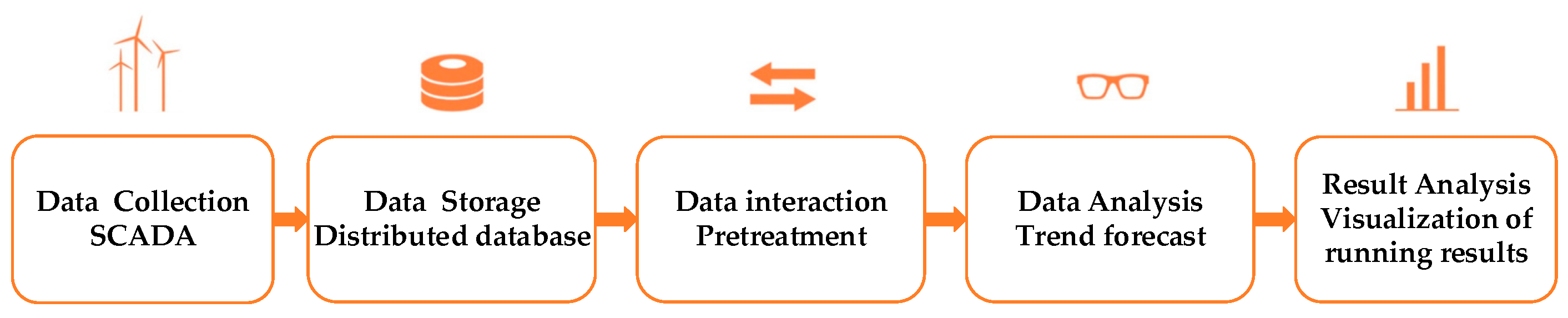
The key technologies of power big data include the following five parts: data acquisition, data storage, data preprocessing, data analysis, and data visualization. The five key parts of wind power big data technologies are shown in Figure 1. In the Figure 1, SCADA means supervisory control and data acquisition.

The acquisition and storage of data is the basis for an in-depth understanding of the operational status of wind turbines as contained in wind power big data; data preprocessing is a prerequisite for data analysis [4,5]; data analysis is the key to obtaining valuable information from massive data [6,7,8,9]; and data visualization is an intuitive and effective method of data presentation. Data preprocessing refers to the review, screening, sorting, transformation, statute, summary, and other processing done before the collected data is processed [10]. Unprocessed data obtained after data collection often have some problems. After preprocessing of data, it is possible to select and extract appropriate features for model training.

In terms of data preprocessing, Wang et al. [11] used data preprocessing techniques and swarm intelligence optimization algorithms to analyze wind speeds for wind energy potential assessment and prediction problems. Niu et al. [12] proposed a combined model for wind speed prediction, including a set of empirical mode decompositions of adaptive noise and a multi-target locust optimization algorithm. Jiang et al. [13] proposed a new hybrid model combining the de-drying method and an optimization algorithm with prediction technology for various unstable factors in complex power systems. Tian et al. [14] studied the accuracy of photovoltaic (PV) power prediction data, and proposed the processing of meteorological data by wavelet decomposition and principal component analysis. Malvoni et al. [15] proposed a cloud segmentation optimal entropy algorithm for the identification of unit anomaly data. Azimi et al. [16] proposed a new time-based K-means clustering method, including discrete wavelet transform, harmonic analysis, and multi-layer perceptual neural network methods, and developed a cluster selection method to determine the optimal training cluster. Zhao et al. [17] studied the feature reduction analysis of wind-induced anomaly data, and integrated the quadrilateral method and density-based clustering method to eliminate sparse outliers. Ye et al. [18] used the adjacent spatial correlation to establish an outlier identification algorithm based on the probabilistic wind farm power curve for the missing data problem in wind farm time series power data.

In terms of data analysis, Renani et al. [19] proposed a new backtracking algorithm for crossover and mutation operators for the problem of wind power prediction, and compared the advantages of an adaptive neuro-fuzzy inference system and other data mining algorithms. Zameer et al. [20] proposed a ML-STWP-based, machine-learning-based short-term wind energy prediction method for short-term wind power forecasting problems, and applied feature selection and regression learning techniques to wind power forecasting. Yuan et al. [21] proposed a hybrid model of the least squares support vector machine and gravity search algorithm for wind farm output power prediction. Abdoos et al. [22] used variational mode decomposition to decompose the time series for the wind power data prediction problem, and then used the Gram–Schmidt orthogonalization to eliminate the redundancy. Finally, the extreme learning machine algorithm was used to train the features.

The above research has mainly been aimed at the cleanup of bad data in wind power big datasets, and the recovery of missing data in the wind speed–power model. Atmospheric dynamics and detailed weather data such as wind direction, wind speed, atmospheric pressure, and air density also have important impacts on the operating state of wind farms, but they have not been paid much attention. Research on data reduction processing with such a large variety of data is also insufficient.

In this paper, a wind power data preprocessing method based on t-SNE has been proposed to reduce the dimensionality of the collected numerical weather prediction. The main work and problems of this paper are as follows:

(1)

Applying the data dimensionality reduction algorithm of t-SNE to the preprocessing of numerical weather prediction (NWP) data of wind farms, and comparing this with the principal component analysis algorithm, the superiority of the algorithm was proven. A long short-term memory network (LSTM) network was used to predict the data after the dimension reduction using t-SNE and the original historical data, which proved that the method improves the prediction accuracy.

(2)

Based on this, a wind farm visualization platform was established to display various types of data.

2. Preprocessing Algorithm

2.1. Normalized Processing

Assuming that the dataset has 2 dimensions, first calculate the influence of the zero mean difference and the covariance. The data after zero mean transformation is:

$$\{\begin{array}{c}{x}^{\prime }=x-\overline{x}\\ y^{\prime }=y-\overline{y}\end{array}$$

(1)

The covariance of the new data is:

$${\sigma }_{xy}^{\prime }=\frac{1}{n}{\displaystyle \sum _{i=1}^n\left(x_i^{\prime }-{\overline{x}}^{\prime }\right)}\left(y_i^{\prime }-{\overline{y}}^{\prime }\right)$$

(2)

${\overline{x}}^{\prime }=0$, ${\overline{y}}^{\prime }=0$, therefore:

$${\sigma }_{xy}^{\prime }=\frac{1}{n}{\displaystyle \sum _{i=1}^n\left(x_i^{\prime }\right)}\left(y_i^{\prime }\right)$$

(3)

The raw data covariance is:

$${\sigma }_{xy}=\frac{1}{n}{\displaystyle \sum _{i=1}^n\left(x_i-\overline{x}\right)}\left(y_i-\overline{y}\right)=\frac{1}{n}{\displaystyle \sum _{i=1}^n\left(x_i^{\prime }\right)}\left(y_i^{\prime }\right)$$

(4)

Therefore:

$${\sigma }_{xy}^{\prime }={\sigma }_{xy}$$

(5)

After the variance is normalized, we have:

$$\{\begin{array}{c}{x}^{″}=\frac{x-\overline{x}}{{\sigma }_x}\\ y^{″}=\frac{y-\overline{y}}{{\sigma }_y}\end{array}$$

(6)

After the variance is normalized, the covariance is as shown in Equation (7).

$${\sigma }_{xy}^{″}=\frac{1}{n}{\displaystyle \sum _{i=1}^n\left(\frac{x-\overline{x}}{{\sigma }_x}\right)}\left(\frac{y-\overline{y}}{{\sigma }_y}\right)=\frac{{\sigma }_{xy}}{{\sigma }_x{\sigma }_y}$$

(7)

The min–max normalization method is used for calculation, and the result of the linear function transformation is:

$$\{\begin{array}{c}{x}^{\prime }=c_x\cdot x\\ y^{\prime }=c_y\cdot y\end{array}$$

(8)

Calculate the covariance as:

$${\sigma }_{xy}^{″}=\frac{1}{n}{\displaystyle \sum _{i=1}^n\left(c_x\cdot x_i-c_x\cdot \overline{x}\right)}\left(c_y\cdot y_i-c_y\cdot \overline{y}\right)=c_x{c}_y{\sigma }_{xy}$$

(9)

2.2. t-SNE Dimensionality Reduction Algorithm

2.2.1. Introduction to t-SNE Algorithm

t-distributed stochastic neighbor embedding (t-SNE) is a nonlinear machine learning algorithm for dimensionality reduction. It is an improvement of the stochastic neighbor embedding (SNE) [23] proposed by Laurens van der Maaten and Geoffrey Hinton. It is very suitable for high-dimensional data dimensionality reduction to 2D or 3D for visualization. The essence of the process is mapping of the similarity between data points in low-dimensional space to high-dimensional space.

2.2.2. Basic Principles and Derivation of the SNE Algorithm

SNE maps data points to probability distributions by affine transformation. From a mathematical point of view, it can be understood that SNE first converts the Euclidean distance into a conditional probability to express the similarity between points.

Given N high-dimensional data $x_1,x_2,\dots ,x_N$, we first construct a conditional probability $p_{ji}$ proportional to the similarity between $x_i$ and $x_j$, using the calculation formula Equation (10).

$$p_{ji}=\frac{\exp \left(-{\Vert x_i-x_j\Vert }^2/\left(2{\sigma }_i^2\right)\right)}{{\displaystyle {\sum }_{k\ne i}\exp \left(-{\Vert x_i-x_k\Vert }^2/\left(2{\sigma }_i^2\right)\right)}}$$

(10)

In the formula, ${\sigma }_i^{}$ is the Gaussian function variance of data point $x_i$.

For low dimensions $y_i$ and the variance of the Gaussian distribution as $\frac{1}{\sqrt{2}}$, $q_{ji}$ indicates the similarity between two points, as defined in Equation (11):

$$q_{ji}=\frac{\exp \left(-{\Vert x_i-x_j\Vert }^2\right)}{{\displaystyle {\sum }_{k\ne i}\exp \left(-{\Vert x_i-x_k\Vert }^2\right)}}$$

(11)

As with Equation (10), we assume that $p_{ji}=0$. If $y_i,y_j$ precisely retain the probability distributions of $x_i,x_j$, it indicates a better dimension reduction effect, from which Equation (12) is established:

$$p_{ji}=q_{ji}$$

(12)

As can be seen from the above, the goal of t-SNE is to find a different way of expressing data that can minimize $p_{ij}$ and $q_{ji}$. By optimizing the distance between these two probability distributions $p_{ij}$ and $q_{ji}$, namely KL scatter (Kullback–Leibler divergences), the objective function is given by Equation (13):

$$C={\displaystyle \sum _{i}KL\left(P_i\Vert Q_i\right)}={\displaystyle \sum _i{\displaystyle \sum _j{p}_{ji}\log \frac{p_{ji}}{q_{ji}}}}$$

(13)

In Equation (13), $P_i$ represents the conditional probability distribution of its data points after $x_i$.

Different points have different ${\sigma }_i$, and the entropy of $P_i$ increases as ${\sigma }_i$ increases. SNE uses the concept of perplexity to represent the best $\sigma$ by binary search. The confusion is:

$$prep\left(P_i\right)=2^{H\left(P_i\right)}$$

(14)

In Equation (14), $H(P_i)$ is the entropy of $P_i$:

$$H\left(P_i\right)=-{\displaystyle \sum _j{p}_{ji}{\log }_2}{p}_{ji}$$

(15)

The physical interpretation of confusion is the number of valid neighbors near a point. After determining the value of $\sigma$, the problem becomes a solution to the gradient. Therefore, the gradient formula of the objective function of t-SNE can be derived as shown in Equation (16):

$$\frac{\delta C}{\delta y_i}=4{\displaystyle \sum _j\left(p_{ij}-q_{ij}\right)}\left(y_i-y_j\right){\left(1+{\Vert y_i-y_j\Vert }^2\right)}^{-1}$$

(16)

Generally, the Gaussian distribution under a small $\sigma$ is used for initialization. In order to speed up the optimization process and avoid falling into the local optimal solution, a large momentum is needed in the gradient update, that is, the parameter update needs to introduce the gradient accumulating term of the previous gradient accumulation. The parameter update formula is Equation (17):

$$Y^{\left(t\right)}=Y^{\left(t-1\right)}+\eta \frac{\delta C}{\delta Y}+\alpha \left(t\right)\left(Y^{\left(t-1\right)}-Y^{\left(t-2\right)}\right)$$

(17)

In Equation (17), $Y^{(t)}$ represents a solution of iteration t times, $\eta$ represents a learning rate, and $\alpha (t)$ represents a momentum of iteration t times.

2.2.3. t-SNE Principle and Derivation

t-SNE uses the t-distribution in low-dimensional space to characterize the similarity between two points. As can be seen from Figure 2, the red line represents a normal distribution and the blue dashed line represents a t-distribution. Due to the difference in the probability distributions of the normal distribution and the t-distribution, the t-distribution has a longer and longer tail effect than the normal distribution. Therefore, in the high-dimensional space where the data values are relatively compact, the data distribution after the dimensionality reduction can be made larger by using the t-distribution.

As seen in Figure 2a, in the absence of outliers, the t-distribution can better describe the edge data; as can be seen from Figure 2b, the t-distribution can better reflect the probability distribution of the data in the presence of outliers. The smaller distances are larger than in the normal distribution after mapping, which captures the overall characteristics of the data.

The $q_{ij}$ changes after using the t-distribution can be shown by Equation (18):

$$q_{ij}=\frac{{\left(1+{\Vert y_i-y_j\Vert }^2\right)}^{-1}}{{\displaystyle \sum _{k\ne l}\left({\left(1+{\Vert y_i-y_j\Vert }^2\right)}^{-1}\right)}}$$

(18)

In addition, in the computational time complexity, since the t-distribution is a linear sum of Gaussian distributions, it does not increase the time complexity. The post-gradient is optimized by t-distribution, as in Equation (19):

$$\frac{\delta C}{\delta y_i}=4{\displaystyle \sum _j(p_{ij}-q_{ij})}(y_i-y_j){(1+{\Vert y_i-y_j\Vert }^2)}^{-1}$$

(19)

According to the derivation of the above algorithm, after summarizing, the flow chart of the t-SNE algorithm as shown in Figure 3 can be obtained. The program can then be implemented according to the steps of the algorithm flow chart.

3. Weather Forecast Data Preprocessing Scheme and Application

3.1. Composition of Wind Farm Operation Data

Classified by its electrical connection and hardware configuration, wind power big data can be divided into three sources: wind farms, wind turbines, and system access points. The composition of wind power big data is shown in Figure 4. In Figure 4, AGC means automatic generation control, AVC means automatic voltage control, STATCOM means static synchronous compensator.

Wind farm big data is composed of primary equipment data, secondary equipment data, and equipment temperature measurement data; wind turbine big data is composed of electrical quantity data, mechanical quantity data, and other data; power system access point big data mainly includes power flow data, AGC, AVC, STATCOM, etc.

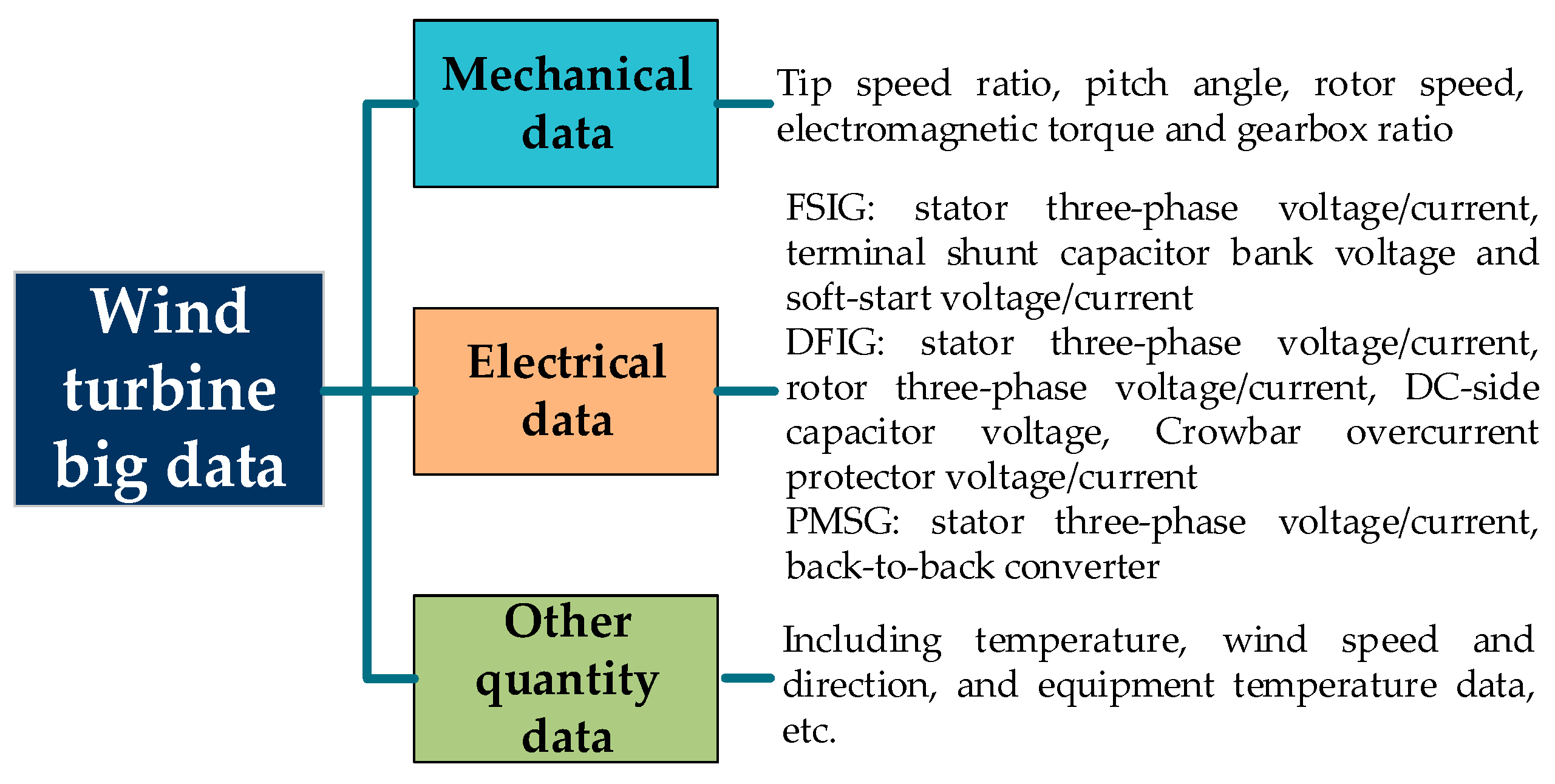
The object of this paper is the preprocessing of wind farm NWP data, which is part of the wind turbine big data. As shown in Figure 5, the wind turbine big data mainly includes wind turbine mechanical quantity data, electrical quantity data, and other data including NWP. The mechanical data and electrical data have lower dimensionality and are important operational data, and have no need for dimensionality reduction; NWP data has a high dimensionality which must be considered, so dimension reduction processing must be considered. The dimensionality-reduced data can be applied to the analysis of various problems, including forecasting, running scheduling, and so on.

For the prediction of wind power output, the current research focused on the wind speed–power model. However, considering only the influence of wind speed on power, other indicators related to power output may be ignored, resulting in a decrease in prediction accuracy. Detailed NWP data such as wind direction, wind speed, atmospheric pressure, and air density of wind farms are used as references for dimension reduction processing, which plays an important role in wind power forecasting and operation scheduling.

3.2. Numerical Weather Data Acquisition and Processing Steps

Numerical weather forecast data has a large number of meteorological indicator variables. The processing method used to date is to select meteorological indicator variables according to experience, but the accuracy of selecting meteorological indicators by experience alone cannot be guaranteed. In addition, low correlation or redundant variables will also adversely affect the cost and time of prediction. In order to improve the efficiency of the model, the N-dimensional data were reduced by the t-SNE dimensionality reduction method.

The purpose of preprocessing wind power data is to normalize, reduce dimensionality, and predict the error of the collected NWP data. The specific implementation steps are as follows:

(1)

The operating status of N fans is measured by various sensors installed on the fan and uploaded to the main station of the wind airport.

(2)

The dimension equivalent of each dimension of the collected data is calculated according to Equations (1)–(10) to avoid the influence of different dimensions.

(3)

According to Equations (11)–(19), the dimensionality of the different indicators in the NWP data is reduced to reduce the redundancy of the phase data.

(4)

The effectiveness of the preprocessing is verified by using the LSTM network for power prediction.

(5)

Visualize the forecast data and historical data.

4. Case Analysis

4.1. Data Source

The sample data used in this paper were from the data segment collected by a wind turbine. The sampling start time was 13:33 on 6 August 2013, and a total of 2.4 million pieces of data were collected. After eliminating the missing variables, the NWP data has 22 remaining dynamics, pressure, temperature, humidity, wind speed, and wind direction at different heights, as shown in

Table 1. Numerical weather prediction NWP variables.

Number of Variables	Index	Shorthand	Unit
1	Air pressure	p	mbar
2	Air temperature	T	degC
3	Thermodynamic temperature	Tpot	K
4	Relative humidity	rh	%
5	Relative pressure	VPact	mbar
6	Absolute humidity	sh	g/kg
7	Air density	rho	g/m3
8	Minimum wind speed	minWs	m/s
9	Rainfall	TP	mm
10	Photosynthetically active radiation	PAR	µmol/m/s
11	Logarithmic temperature	Tlog	degC
12	Carbon dioxide concentration	CO2	ppm
13	Maximum wind speed	maxWs	m/s
14	10 m wind speed	wv	m/s
15	10 m wind direction	wd	deg
16	10 m wind level	ws	/
17	20 m wind speed	wv	m/s
18	20 m wind direction	wd	deg
19	20 m wind rating	ws	/
20	30 m wind speed	wv	m/s
21	30 m wind direction	wd	deg
22	30 m wind rating	ws	/

.

As can be seen from Table 1, the dimensionality of the NWP data was very high, and it was not possible to determine whether each feature affects the operating state of the wind farm. If the data were subsequently input into the prediction model without processing, too many data would not only lead to a large increase in computation time, but would also affect the ability of the model to express features. Therefore, it was necessary to select valuable features from the appropriate algorithms. In this part, the t-SNE method introduced above was used for feature selection, and compared with the PCA dimensionality reduction algorithm.

4.2. Wind Power Big Data Dimensionality Reduction Based on t-SNE Algorithm

In order to remove the noise of the NWP samples and visually reflect the characteristics of wind farm meteorological data in low-dimensional space, the sample set was reduced from 22 dimensional to 2 dimensional space using the t-SNE algorithm, the confusion was set to 20, and iteration was set to 5000 times. The effect of confusion was to balance the weights of the t-SNE local transformation and the global transformation. It can be understood that the confusion was used to set the number of adjacent points of each point. The greater the confusion setting, the more attention is paid to the global data distribution. Usually, the confusion parameter is roughly equal to the number of neighbors needed. In this paper, it was determined based on the NWP variables. The number of iterations was based on the parameters recommended by the authors in the literature [23].

We selected 3000 data from a single day to show the dimensionality reduction results of the t-SNE algorithm, as shown in Figure 6. The dots in the figure represent data points, and the different colors represent different variables.

As shown in Figure 6, the data of the input NWP were color-coded according to the number of data categories in the default series of RGBA, RGBA is the color space representing red green blue and alpha. The t-SNE algorithm was able to clearly represent all data points in a 2 dimensional space, and most of the data points of different features exhibited a short-line structure of one or several segments. The t-SNE algorithm clearly separated the different categories of data.

At the same time, it can be seen from Figure 6 that when the algorithm was used to reduce the original data to 2 dimensions, some data points overlapped, for example, the red and blue in the figure overlap, making them more difficult to distinguish. Therefore, the following attempt was to to reduce the original sample set to the three dimensional subspace using the t-SNE algorithm. The confusion was set to 20 and iteration was set to 5000 times. We again selected 3000 data to show the dimensionality reduction results, as shown in Figure 7. The colors of the input data were color-coded according to the format of “RdYlGn”, which is the order from red to green.

In order to verify the generalization of the t-SNE model, the meteorological data segment of this wind farm at other times was used as the experimental object, and the sampling start time was 8 August 2013. After the data were input into the model using the same preprocessing method, the dimensionality reduction visualization that resulted is shown in Figure 8.

It can be seen from the above simulation results that the t-SNE algorithm could clearly represent all data points in three dimensional space. Most data points presented a one- or several-segment short-line segment structure that reflected the temporal continuity of weather changes. It can be seen that dots of different colors represent different features that were distinctly distinguished in three dimensions. The simulation results demonstrated the effectiveness of the t-SNE algorithm in processing meteorological data in wind farm operating data.

Analysis of the distance relationship between data points does not provide quantitative information about the data. Therefore, the purpose of the t-SNE dimensionality reduction method is mainly to visualize the data, so that we can have a macroscopic understanding of the data patterns that need to be mined. For a certain set of data, if t-SNE performs well on the segmentation feature, it is highly probable that a machine learning method that projects this set of data into different categories will be found. Conversely, if t-SNE is generally represented on segmentation features, such as in the case of class overlaps, then a more complex model needs to be built.

4.3. Comparison with the PCA Algorithm for Dimensionality Reduction

The idea of principal component analysis is to find one or several projection directions so that the variance of the original data samples after projection is maximized. The original m-dimensional features are projected onto a new n-dimensional space, which is characterized by the principal component. The main evaluation method of principal component selection is to use variance. The larger the variance of new features, the more information contained in this feature can be reflected. Therefore, the percentage of contribution of cumulative variance is calculated to select the principal component.

Assuming that the sample set $X=\left\{x_1,x_2,\dots ,x_m\right\}$ satisfies the centralization, it is assumed that the new coordinate system after the projection transformation is $\left\{w_1,w_2,\dots ,w_d\right\}$, where $w_i$ is the standard orthogonal basis vector and ${\Vert w_i\Vert }_2=1$. The projection of a data point $x_i$ in the new coordinate system $\left\{w_1,w_2,\dots ,w_d\right\}$ is $W^T{x}_i$. If the projection of the data points in the original sample set can be effectively separated under this new coordinate system, the variance of the different sample data points in the new coordinate system is ${\displaystyle \sum _i}{W}^T{x}_i{x}_i^{T}W$, so the optimization goal is to maximize this variance:

$$\{\begin{array}{c}\underset{w}{\max }\mathrm{tr}\left(W^{T}X{X}^{T}W\right)\\ \mathrm{s}.\mathrm{t}.\begin{array}{c}\end{array}{W}^{T}W=1\end{array}$$

(20)

For Equation (20), the Lagrangian multiplier method is used, giving:

$$X{X}^{T}W=\lambda W$$

(21)

Therefore, it is only necessary to perform eigenvalue decomposition on the covariance matrix and sort the obtained eigenvalues: ${\lambda }_1\ge {\lambda }_2\ge \dots \ge {\lambda }_m$. Generally, a dimension with a cumulative contribution rate of about 75% to 95% is selected as the reference dimension after PCA dimensionality reduction.

The variance contribution rate and the cumulative variance contribution rate are, respectively:

$${\eta }_i=\frac{100\%{\lambda }_i}{{\sum }_m{\lambda }_i}$$

(22)

$${\eta }_{\sum }\left(p\right)={\displaystyle \sum }_i^p{\eta }_i$$

(23)

The eigenvectors corresponding to the first x eigenvalues constitute the solution of principal component analysis $W=\left(w_1,w_2,\dots ,w_x\right)$.

In order to compare the dimensionality reduction effect of the t-SNE and PCA algorithms, the data of wind farm meteorological data segment 1 were reduced to 2D, 3D, 5D, and 8D space, and credibility was used as the evaluation standard. Credibility indicates the retention of the local structure of the original structure of the data when dimension reduction to low-dimensional space is carried out. The size range of credibility is [0,1]. The greater the credibility, the better the data retention, and the lower the credibility, the worse the data retention after dimension reduction. The mathematical definition of credibility is given by Equation (24).

$$T(k)=1-\frac{2}{nk\left(2n-3k-1\right)}{\displaystyle \sum _{i=1}^n{\displaystyle {\sum }_{j\in u_i^{}}\left(r\left(i,j\right)-k\right)}}$$

(24)

In Equation (24), $r(i,j)$ represents the rank of the low-dimensional data points $j$, determined according to the pairwise distance between the low-dimensional data points, and $U_i^k$ represents the set of neighbor data points $k$ in the low-dimensional space. The following will be used to compare the reliability of high-dimensional data to 2, 3, 5, and 8 dimensions using PCA and t-SNE.

Table 2. Comparison of trustworthiness of low-dimensional representations of the data set. PCA—principal component analysis.

Dimension	PCA	t-SNE
2	0.918	0.921
3	0.970	0.975
5	0.975	0.983
8	0.977	0.989

and Figure 9 show the comparison of the reliability of the data after dimension reduction using the t-SNE algorithm and the PCA method. Through the graph, it can be seen that t-SNE gave a significant improvement in the dimensionality reliability of the experimental low-dimensional space compared with PCA, and t-SNE basically retained the time-series characteristics of the original data. PCA means principal component analysis

4.4. Comparison of Wind Speed Prediction Before and After Data Preprocessing

Here, the long-short-term memory (LSTM) was selected as the wind speed prediction model to evaluate the effect of the wind power data preprocessing. As a complex nonlinear unit, LSTM uses a deeper neural network to reflect long-term memory effects and has deep learning ability [24,25].

The preprocessed data were divided into training data and test data. Among them, 1300 pieces of data are used as training data, and the remaining 500 pieces of data are used as test data.

In the error analysis of the prediction results, it is often evaluated by two evaluation indicators: mean absolute percentage error (MAPE) and root mean square error (RMSE). The error calculation formula is given by reference to Equations (25) and (26), respectively.

$${\epsilon }_{MAPE}=\frac{1}{n}{\displaystyle \sum _{i=1}^n\frac{\left|{\widehat{P}}_N(i)-P_N(i)\right|}{P_N(i)}}\times 100\%$$

(25)

$${\epsilon }_{RMSE}=\sqrt{\frac{1}{n}{\displaystyle \sum _{i=1}^n}{({\widehat{P}}_N(i)-P_N(i))}^2}$$

(26)

In Equations (25) and (26), $P_N(i)$ and ${\widehat{P}}_N(i)$ (i = 1, 2, 3, …, n) are the actual measured and predicted values of the data point i, respectively, and n represents the length of the data used for verification.

Table 3. Error analysis of the forecasting result.

Index	Type of Data	${\mathit{\epsilon }}_{\mathit{M}\mathit{A}\mathit{P}\mathit{E}}$ (%)	${\mathit{\epsilon }}_{\mathit{R}\mathit{M}\mathit{S}\mathit{E}}$
Active power	Preprocessed data	0.603	2098.866
	historical data	0.711	2293.650
Phase current	Preprocessed data	3.1589	73.358
	historical data	3.722	80.577
Phase voltage	Preprocessed data	2.224	32.68
	historical data	2.517	37.955

shows the prediction results of the wind farm data through the preprocessing method of this paper and the direct use of the original data. It can be seen from Table 3 that the prediction results ${\epsilon }_{MAPE}$ and ${\epsilon }_{RMSE}$ after preprocessing by t-SNE were reduced compared with the prediction results using historical data, which effectively improved the prediction accuracy. The results also show that after the dimension reduction preprocessing, the analysis of less relevant invalid variables can be avoided, and only the highly correlated useful variables were retained, which helps to improve the prediction performance of the LSTM model. In addition, after using the dimensionality reduction preprocessing method of this paper, the input variables were much fewer than the original, which is conducive to large-scale data calculation. MAPE is mean absolute percentage error and RMSE means root mean square error.

4.5. Visualization Platform Implementation

We designed a visualization system for statistical and real-time status monitoring of wind power big data. In order to display relevant information in a timely manner, the platform uses Grafana as a visualization tool and the timing database InfluxDB as a data storage container. In the experimental part, the Python language was used to implement various functions, including client and server building, reading, and writing to InfluxDB.

InfluxDB is backed by Norwest Venture Partners, Sapphire Ventures, Battery Ventures, Trinity Ventures, Mayfield, Harmony Partners, Sorenson Capital, Bloomberg Beta and Y Combinator, its location is San Francisco, CA 94103, USA. Grafana is created by raintank co-founder Torkel Odegaard and located in San Francisco, USA. Python is created by Guido van Rossum and managed by Python software foundation, located in Beaverton 97008, USA.

4.5.1. System Architecture and Implementation Process

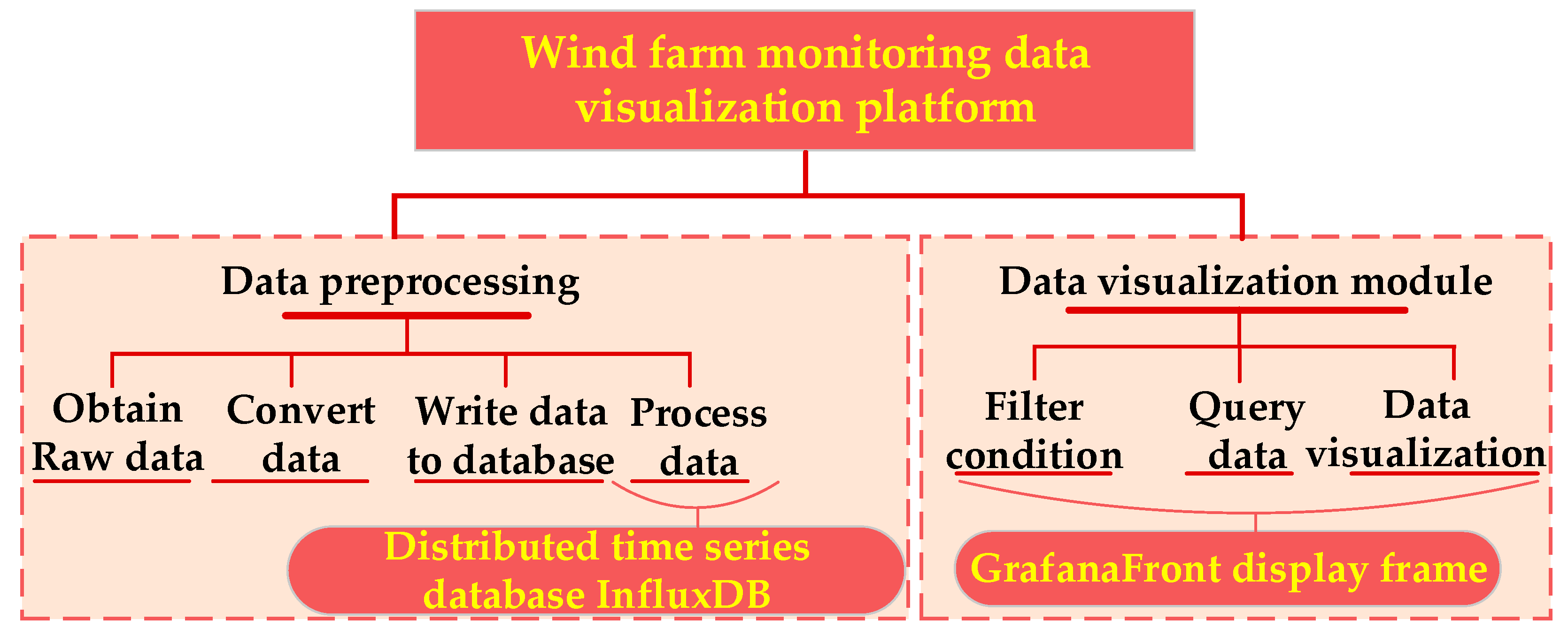
The overall architecture of the wind farm monitoring data visualization platform is shown in Figure 10. The visualization platform was mainly composed of a data processing module and a data visualization module. The data processing module was responsible for processing the raw data and importing it into the database. The visualization module was responsible for reading and aggregating the data and visualizing it. The data visualization module also included data query and data aggregation functions. Through these two functions, the wind farm monitoring data visualization platform can be realized.

The visualization implementation process is shown in Figure 11. The data were processed and filtered, transformed into visually expressible geometric data by mapping, and finally rendered into user-visible image data.

4.5.2. Visualization Platform Implementation

The data visualization platform included the following three modules: a data processing module, a data aggregation module, and a data visualization module. The data processing module converted the wind power data in the form of a csv file into Json format and wrote it to the InfluxDB database in batches. The data aggregation module compressed aggregated operational data through the data retention function and continuous query (CQ) function provided by InfluexDB. Data visualization module: Connect the data in the InfluxDB database to Grafana and select the appropriate visualization panel to visualize meteorological data such as precipitation, pressure, temperature, humidity, and wind speed and direction.

Currently, there are six types of panels, including Graph, Singlestat, Heatmap, Dashlist, Table, and Text. The visualization panel for each meteorological factor of the wind farm is shown in Figure 12.

5. Conclusions

In this paper, the preprocessing links in wind farm big data mining were studied, and data preprocessing methods were discussed and applied. The t-SNE algorithm was used to preprocess and analyze numerical weather prediction (NWP) data. The main conclusions are as follows:

(1)

Due to the large size of meteorological indicator variables in NWP data, the traditional feature selection method is no longer effective. For this reason, the t-SNE algorithm was used to reduce the NWP data. Using actual NWP data collected by a wind farm, the experiment proved that t-SNE can better preserve the local similarity of sample points in the original high-dimensional space in 2 dimensional space; the t-SNE data preprocessing method improved the computational efficiency of the subsequent data analysis model while ensuring accuracy.

(2)

By comparing two different data preprocessing methods, t-SNE and PCA, it was found that the dimensionality reliability of t-SNE was slightly better than the PCA dimensionality reduction method in each low-dimensional space of the experiment; the data preprocessing results of the t-SNE and PCA algorithms were applied to wind power prediction based on a deep learning LSTM network, which proved that the preprocessed data had better prediction accuracy.

(3)

The wind farm monitoring data visualization platform consisted of a data processing module, a data aggregation module, and a data visualization module, able to realize the visualization of the massive data recorded during the operation of the wind farm. It not only provides important understanding of the operating state of the wind farm, but also provides a basis for the construction of subsequent trend prediction models.