Recurrent Neural Networks Based Photovoltaic Power Forecasting Approach

Abstract

The intermittency of solar energy resources has brought a big challenge for the optimization and planning of a future smart grid. To reduce the intermittency, an accurate prediction of photovoltaic (PV) power generation is very important. Therefore, this paper proposes a new forecasting method based on the recurrent neural network (RNN). At first, the entire solar power time series data is divided into inter-day data and intra-day data. Then, we apply RNN to discover the nonlinear features and invariant structures exhibited in the adjacent days and intra-day data. After that, a new point prediction model is proposed, only by taking the previous PV power data as input without weather information. The forecasting horizons are set from 15 to 90 min. The proposed forecasting method is tested by using real solar power in Flanders, Belgium. The classical persistence method (Persistence), back propagation neural network (BPNN), radial basis function (RBF) neural network and support vector machine (SVM), and long short-term memory (LSTM) networks are adopted as benchmarks. Extensive results show that the proposed forecasting method exhibits a good forecasting quality on very short-term forecasting, which demonstrates the feasibility and effectiveness of the proposed forecasting model.

1. Introduction

Solar energy is a completely free cost and easily accessible source of energy that has proven to be one of the cleanest and most abundant renewable energy sources. Many large-scale solar photovoltaic (PV) plants are widely applied in many countries in the world to reduce environmental pollution and carbon emissions caused by fossil energy [1]. However, the variability of solar energy resources has brought difficulties to electric power grid management with the increase of solar energy penetration rates. Meanwhile, the access of a large number of PV power plants to randomness and intermittency will seriously affect the stable operation of the entire power system [2]. It should be mentioned that PV power forecasting is an important factor in the power system to solve the problem of solar PV power plant optimization planning and modeling. The research in [3] indicates that an accurate forecasting of PV power becomes crucial to improve the power system stability and to ensure an optimal unit commitment and economic dispatch.

In practice, the task of a more accurate solar power forecasting plays a crucial role in the smart grid. In [4], a reliable PV forecasting method provides the necessary predicted input data to the optimization stage for grid-connected PV systems with storage. Simulations show that the efficiency of the predictive schedule depends on the accuracy of the forecasts. With the forecasted values, the actual PV load can be calculated for a multi-objective economic load dispatch to minimize the total operating cost of the distributed network. The online prediction results can also be used to model the various uncertainties of PV power in real-time energy management systems [5]. In [6], deterministic PV generation forecasting is utilized to design an efficient generation controller to achieve an optimal microgrid economic operation. In [7], a solar power forecasting system is used to design the ramp-rate control strategy for large PV systems without energy storage. The PV output power will ensure that it is smoothed in advance because the participation of the forecasting system provides sufficient pre-operation time for the inverter. PV power forecasting results can also help reduce power flows to the grid and improve the self-consumption of PV generated electricity [8]. In addition, the PV power forecasting technology will be widely implemented in the electric vehicle charge-discharge management coordination between home and grid energy management systems [9], the multi-objective optimal design of hybrid renewable energy system [10] and the robust planning of the electric vehicle charging facilities [11]. Therefore, a good PV power forecasting method is needed to promote the future application of solar energy.

In recent years, PV power generation has attracted great interest from researchers around the world. The PV prediction methods can be classified into three categories: the physical method, statistical method, and artificial intelligence method [12]. The physical method obtains meteorological and geological parameters through numerical weather prediction (NWP), satellite remote sensing measurement and ground measurement devices. But service facilities with appropriate and frequent calibration are required [13]. The statistical method is a data-driven approach that extracts features from historical samples to predict the future behavior of PV via an error minimization. The key to accurately predict PV output power is the quality of historical samples [14]. Meanwhile, artificial intelligence techniques have become an excellent tool for wind generation and PV generation [15,16] and can solve the problem of a non-linear function estimation [17]. For example, the neural networks can be used to model the characteristics of traditional silicon-based PV modules; then, such networks, together with the intelligent algorithmic, are utilized to automatically parametrize the Voltage-Current characteristics of organic PV modules [18]. Meanwhile, the artificial intelligence technology is also playing a key role in the energy domain, such as the control system [19], energy consumption [20], pattern recognition and failure classification [21,22]. In particular, with the rapid development of artificial intelligence algorithms and excellent performance in many fields, it is superior to other models in dealing with non-linear problems with strong uncertainties [23].

Focusing on solar energy prediction by artificial intelligence techniques, many direct forecasting models are generally proposed in the literature. In [15], a novel artificial neural network (ANN) model using statistical feature parameters is proposed for short-term solar irradiance forecasting. In [24], an improved adaptive back propagation neural network (BPNN) prediction model is established to forecast PV power. The forecasting model adapts to time and a changing external environment through the scrolling time window. In [25], the weather conditions are divided into four categories: clear sky, cloudy day, foggy day and rainy day. Then, a general framework based on weather classification data, historical measured power and support vector machine (SVM) is developed to approximate the PV generation prediction model. In [26], an advanced prediction model based on the radial basis function (RBF) neural network is proposed to predict the PV power of the next 24 h. Here, a self-organized map (SOM) is used to classify the weather types from NWP. However, an appropriate mathematical model without complicated calculations is still needed to predict the PV output power. As one of the deep learning algorithms, recurrent neural networks (RNN) has been successfully applied to the smart grid [27]. In [28], the sunshine, radiation intensity, atmospheric pressure, and the temperature before the predicted time step is considered to establish the prediction model, and its forecast error is minimized by RNN. In [29], RNN is used as a good tool for the time series prediction, with a good performance for the solar radiation prediction. The authors in [30] propose the use of the long-short-term memory recurrent neural network (LSTM-RNN) to accurately forecast the output power of PV systems.

In particular in the forecasting approaches, a good approach could directly predict the PV output power based on some prior information or readily accessed data. RNN can remember the power changes between the inter-day because of their recurrent architecture and memory units. Previous studies have proven that the RNN model can discover the inherent abstract features and hidden invariant structures in data from the lowest level to the highest level without complicated calculations. Nevertheless, there is still no published research that considers both the inter-day (and day-to-day) and intra-day (or within-day) information for very short-term PV power forecasting. A natural extension in this context is that: if the forecasting model can utilize the PV power of inter-day and intra-day, it is expected to explore a more accurate prediction performance. Therefore, we originally propose a very short-term forecasting model, based on RNN, that considers both the inter-day and intra-day PV power. Meanwhile, the inter-day data input to RNN model can provide more detailed information for a very short-term PV power prediction. The main contributions of this article are as follows:

(1)

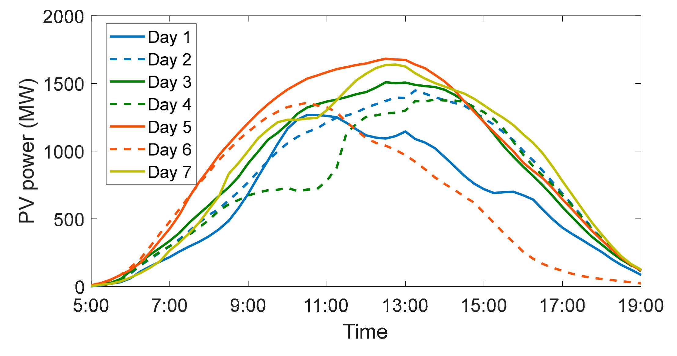
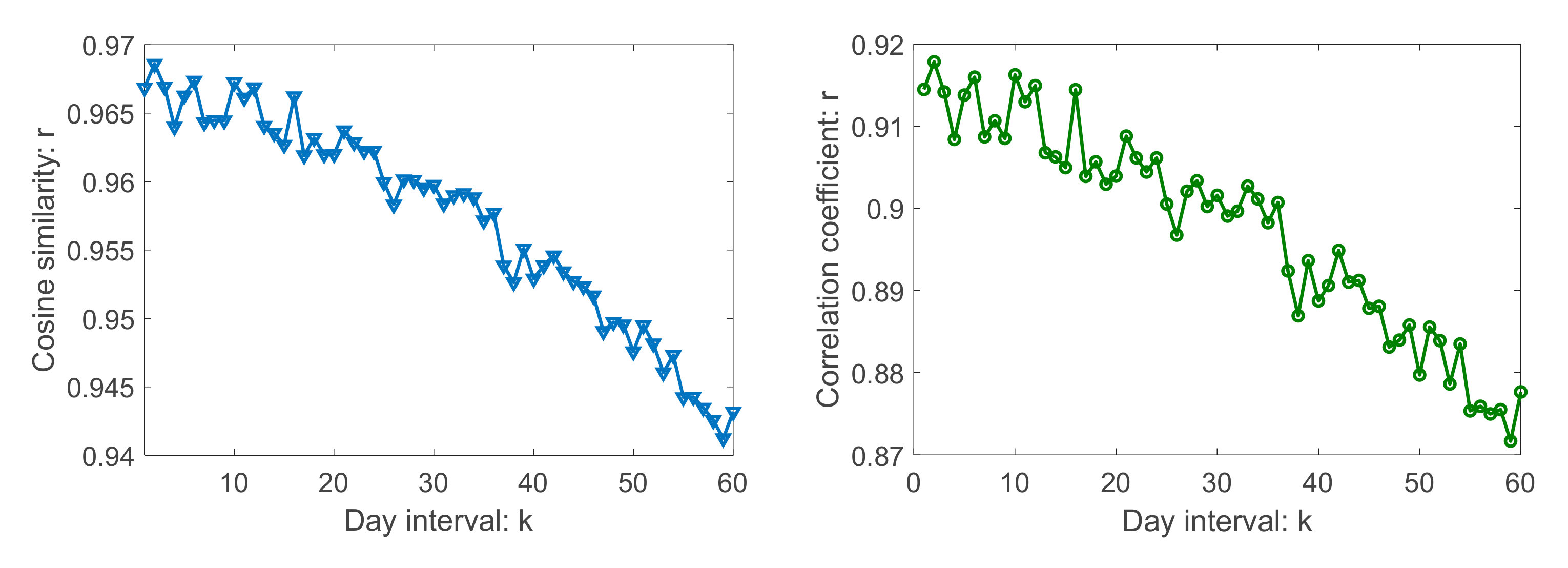
In this paper, the PV power correlation of adjacent days is verified and analyzed.

(2)

The RNN model is introduced and tailored to fully extract high-level non-linear features hidden in the inter-day and intra-day power data.

(3)

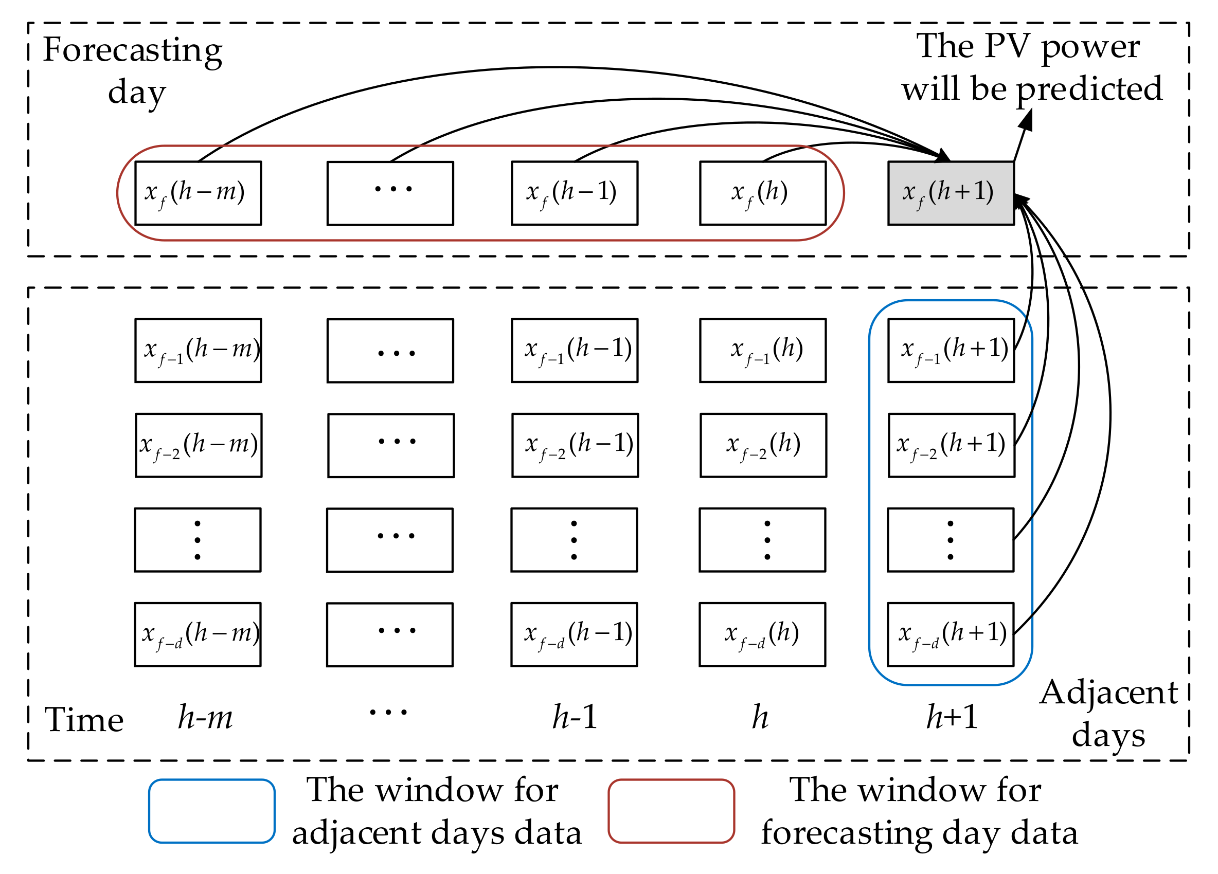
For the first time, a novel PV power forecasting method based on adjacent days and intra-day data is proposed to mitigate the effects of the nonlinearity features that exist in the PV output power series on the prediction accuracy.

The performance is validated using real solar power in Flanders, Belgium. The extensive results show that the proposed method can effectively extract the invariant structures exhibited in the historical PV power data, and accurately predict the output power of PV. The main purpose of this paper is to predict PV power, i.e., to minimize the error between measured power and predicted power. Usually, the measurement error is very small and usually negligible. Therefore, measurement errors are generally not considered in PV power prediction. Consequently, we consider the measured power as the actual PV power in the proposed forecasting model. The paper is organized as follows. Section 2 presents the RNN model. Section 3 presents a point forecasting model based on RNN and the data of the adjacent days. Section 4 gives a case study and discussions. Section 5 presents the conclusions.

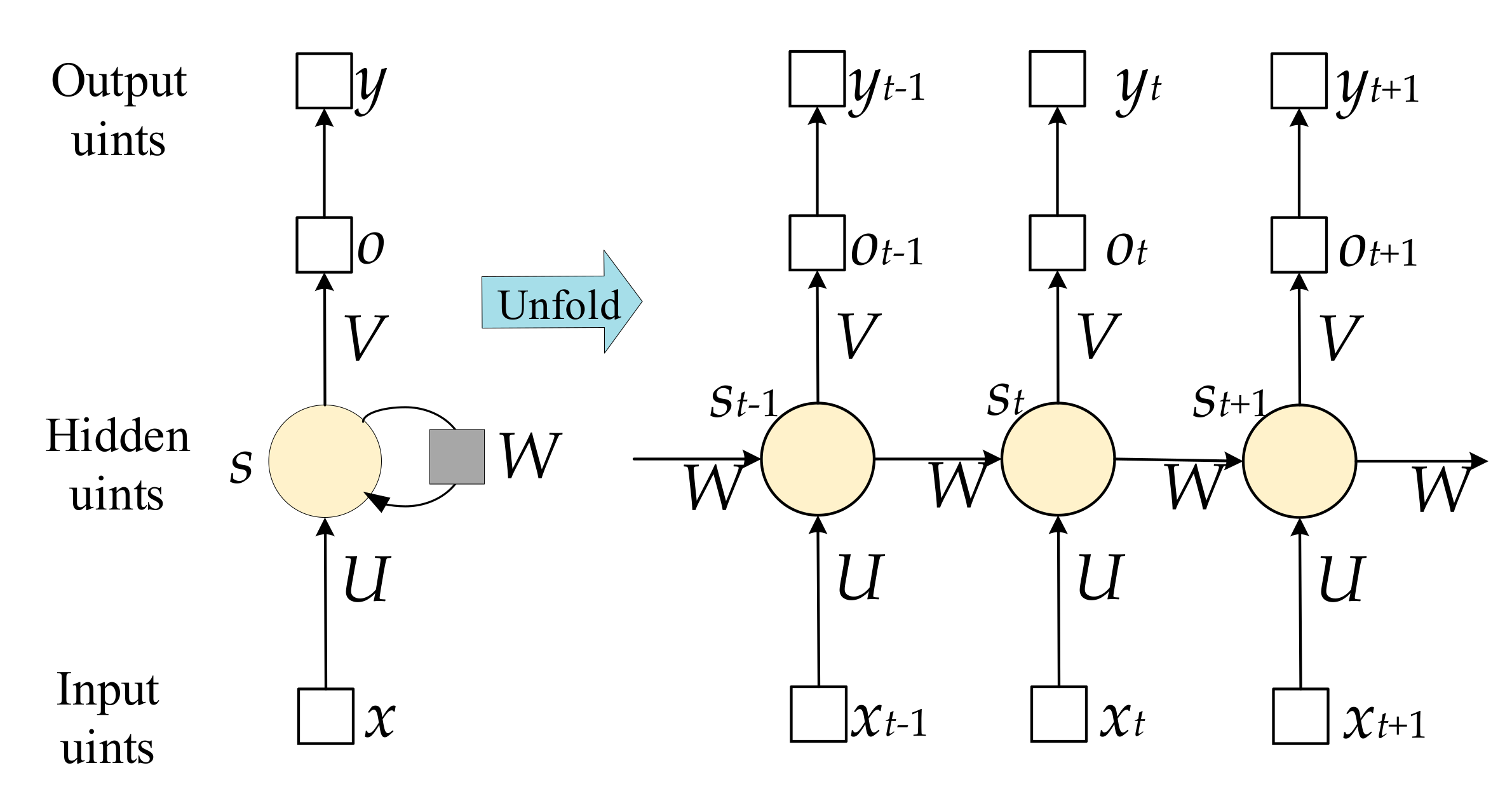
2. Recurrent Neural Networks

2.1. RNN Model

Figure 1 shows the structure of the RNN model. x^t and y^t are the input variable and output variable of the RNN at step t. The hidden state s^t of the RNN model is calculated based on the input x^t at the current step t and the previous hidden state s^t−1 at the step t−1. The mathematical model of RNN is expressed as follows:

$$s^t=f\left((U{x}^t+b)+W{s}^{t-1}\right)$$

(1)

$$o^t=V{s}^t+c$$

(2)

$$y^t=g(o^t)$$

(3)

where $U\in R^{l_x\times l_s}$ is the weight matrix between the input layer and the hidden layer. $W\in R^{l_{\mathrm{s}}\times l_s}$ is the weight matrix between the hidden layer and the hidden layer. $V\in R^{l_o\times l_s}$ is the weight matrix between the hidden layer and the output layer. It can be noted that in Figure 1 the parameter values of the weight matrixes U, W, and V are not changed in the different steps. l_x, l_s and l_o are the numbers of neurons in the input layer, hidden layer and output layer, respectively. s^t is the hidden layer state at step t, and it is the “memory” of the RNN. The parameters b and c are bias vectors. o^t is a temporary variable, and o^t is only determined by the hidden state s^t of the RNN model. f = tanh and g = sigmoid are the activation functions of the hidden layer and the output layer, respectively.

2.2. Parameter Learning Procedures of RNN

To learn the parameters U, V, W, b, and c of the RNN model, the back propagation through time (BPTT) approach is used in this work to calculate the gradient of these parameters [31]. BPTT is a back propagation training algorithm of RNN, which is applied to the sequence data like time series. The BPTT approach works by unrolling all of the input time steps, and the sample errors of RNN are computed and accumulated at each time step. The cost function of RNN can be set as:

$$L={\displaystyle \sum _{t=1}^{\tau }\left(\frac{1}{2}{\displaystyle \sum _{j=1}^{l_o}{({\stackrel{⌢}{y}}_j^t-y_j^t)}^2}\right)}$$

(4)

where L is the total cost of all of the time sequences. Equation (4) indicates that the total cost is just the sum of the sub-costs at each time step. $y_j^t$ and ${\stackrel{⌢}{y}}_j^t$ are the measured value and predicted value, respectively. The hidden state gradient of step t is defined as:

$${\delta }^t=\frac{\partial L}{\partial s^t}$$

(5)

From the RNN model, it can be seen that δ^t is determined by the sub-cost at the current step t and the sub-cost at step t+1. So, δ^t is related to the output temporary variable o^t and the hidden layer state s^t+1.

$$\begin{array}{l}{\delta }^t=\frac{\partial L^t}{\partial o^t}\frac{\partial o^t}{\partial s^t}+\frac{\partial L^{t+1}}{\partial s^{t+1}}\frac{\partial s^{t+1}}{\partial s^t}\\ =V^T({\stackrel{⌢}{y}}^t-y^t)g^{\prime }(o^t)+W^T{\delta }^{t+1}\mathrm{diag}\left(1-{(s^{t+1})}^2\right)\end{array}$$

(6)

where diag(^.) stands for creating a diagonal matrix from a given vector. Since there is no other hidden state after the last step τ, the δ^τ is written as:

$${\delta }^{\tau }=\frac{\partial L}{\partial o^{\tau }}\frac{\partial o^{\tau }}{\partial s^{\tau }}=V^T({\stackrel{⌢}{y}}^t-y^t)g^{\prime }(o^t)$$

(7)

The gradient of network parameters at step t is calculated step by step by back propagation. Then, the gradient of U, V, W, b and c can be expressed by the following formula:

$$\frac{\partial L}{\partial c}={\displaystyle \sum _{t=1}^{\tau }\frac{\partial L^t}{\partial o^t}}\frac{\partial o^t}{\partial c}={\displaystyle \sum _{t=1}^{\tau }({\stackrel{⌢}{y}}^t-y^t)g^{\prime }(o^t)}$$

(8)

$$\frac{\partial L}{\partial V}={\displaystyle \sum _{t=1}^{\tau }\frac{\partial L^t}{\partial o^t}\frac{\partial o^t}{\partial V}}={\displaystyle \sum _{t=1}^{\tau }({\stackrel{⌢}{y}}^t-y^t)g^{\prime }(o^t)}{(s^t)}^T$$

(9)

$$\frac{\partial L}{\partial b}={\displaystyle \sum _{t=1}^{\tau }\frac{\partial L}{\partial s^t}}\frac{\partial s^t}{\partial b}={\displaystyle \sum _{t=1}^{\tau }\mathrm{diag}\left(1-{(s^t)}^2\right){\delta }^t}$$

(10)

$$\frac{\partial L}{\partial W}={\displaystyle \sum _{t=1}^{\tau }\frac{\partial L}{\partial s^t}}\frac{\partial s^t}{\partial W}={\displaystyle \sum _{t=1}^{\tau }\mathrm{diag}\left(1-{(s^t)}^2\right){\delta }^t{(s^{t-1})}^T}$$

(11)

$$\frac{\partial L}{\partial U}={\displaystyle \sum _{t=1}^{\tau }\frac{\partial L}{\partial s^t}}\frac{\partial s^t}{\partial U}={\displaystyle \sum _{t=1}^{\tau }\mathrm{diag}\left(1-{(s^t)}^2\right){\delta }^t{(x^t)}^T}$$

(12)

Obviously, the final gradients of the network parameters are the sum of the sub-gradients at each time step. The gradients of the network parameters can be easily calculated using Equations (2)–(4), (9) and (10). Therefore, the updated rule for these parameters are as follows:

$$b^{n+1}=b^n-\eta \frac{\partial L}{\partial b}$$

(13)

$$c^{n+1}=c^n-\eta \frac{\partial L}{\partial c}$$

(14)

$$V^{n+1}=V^n-\eta \frac{\partial L}{\partial V}$$

(15)

$$W^{n+1}=W^n-\eta \frac{\partial L}{\partial W}$$

(16)

$$U^{n+1}=U^n-\eta \frac{\partial L}{\partial U}$$

(17)

where η is the learning rate of RNN, and the superscript n stands for the iteration times of BPTT. The partial derivatives of the cost function with respect to the disturbance of b, c, V, W and U can be inferred from Equations (8)–(12).

3. Adjacent Days and Intra-day Point Forecasting Model Based on RNN

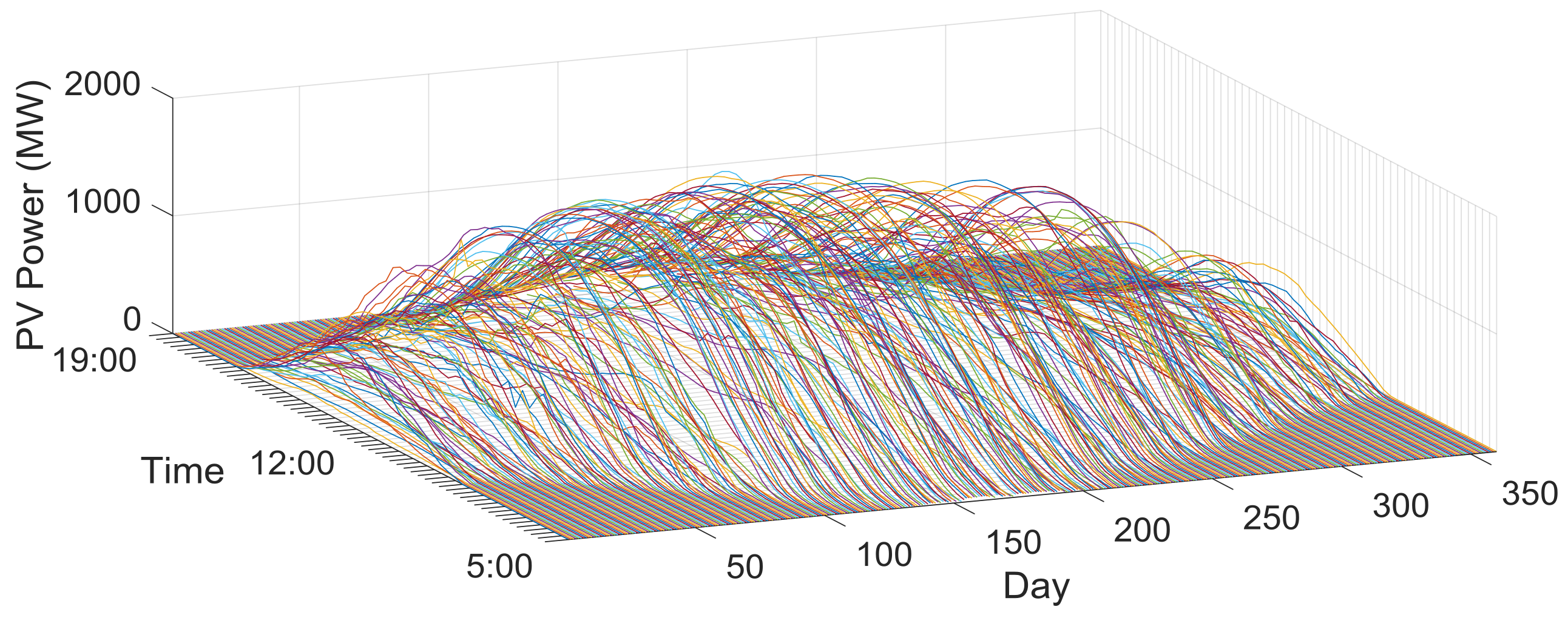
3.1. Adjacent Days and Intra-day Data

In Figure 2, we plot the PV power curves for seven days over a period of time. The unit of PV power is MW, and the historical data is recorded by an electricity transmission system operator in Belgium [32]. From the plots, the PV power of one day is very similar to the PV power of the adjacent days when the weather condition does not change drastically in a short period of time. It can be seen that the PV power of adjacent days can provide more weather information for future PV power forecasting. The PV power of adjacent days with a shorter time interval has a higher degree of similarity. Hence, this paper considers the adjacent power data before the forecasting day for the proposed prediction model.

In Figure 3, we evaluated the correlation of the output power of adjacent days for different k-day intervals. We consider a historical PV power dataset over one year and calculate the average of the performance metrics with k-day intervals. We consider 60 power points of one day, and the daily data covers the time period from 5:00 to 19:00, with a 15-min resolution. For adjacent days, we assume the PV output power for the ith day is P_i = [p_i1, p_i2, …, p_iM] and the jth day output power is P_j = [p_j1, p_j2, …, p_jM]. We assume the ith day is the forecasting day and the jth day is a historical day adjacent to the forecasting day. Here, M is the length of the daily data, and p_i1 is the PV power point at 5:00. Then, we use the cosine similarity [33] and the correlation coefficient [34] as the similarity degree metrics. The cosine similarity will reflect the trend similarity degree of the daily power on the forecasting day and a historical day adjacent to the forecasting day. The correlation coefficient is always used to measure the correlation between the two days. The metrics are defined as follows:

$$c_{ij}=\frac{{\displaystyle \sum _{m=1}^M{p}_{im}{p}_{jm}}}{\sqrt{{\displaystyle \sum _{m=1}^M{p}_{im}^2}}\sqrt{{\displaystyle \sum _{m=1}^M{p}_{jm}^2}}}$$

(18)

$$r_{ij}=\frac{{\displaystyle \sum _{m=1}^M(p_{im}-{\overline{p}}_i)(p_{jm}-{\overline{p}}_j)}}{\sqrt{{\displaystyle \sum _{m=1}^M{(p_{im}-{\overline{p}}_i)}^2{(p_{jm}-{\overline{p}}_j)}^2}}}$$

(19)

$$c_k=\frac{1}{n-k}{\displaystyle \sum _{i=1}^{n-k}{c}_{ij}},r_k=\frac{1}{n-k}{\displaystyle \sum _{i=1}^{n-k}{r}_{ij}}$$

(20)

where i∈[1, …, n-k], j=i+k, m∈[1, …, M], k is an interval value representing the number of days between the ith day and the jth day, n is the number of days in the whole year, p_im is a power point of the ith day, and ${\overline{p}}_i$ is the mean value of the ith daily data. The cosine similarity c_ij can reflect the trend similarity degree of daily power between the ith day and the jth day, independent of their magnitude. The correlation coefficient r_ij is always used to measure the day similarity degree of two days. The metric c_k and r_k are the average values of the cosine similarity c_ij and correlation coefficient r_ij, respectively.

As can be seen from Figure 3, the cosine similarity and the correlation coefficient of the historical day both deteriorate when k increases. The results show that the historical day with a smaller k will have a higher cosine similarity and correlation coefficient. That is, the output power of the adjacent days has a high correlation under a scenario of a short time interval. Hence, the consideration of adjacent days’ data has a positive effect on the PV power forecasting. This forecasting model that takes into account the PV power of adjacent days makes up for the deficiency of PV power forecasting that is only based on intra-day data.

3.2. Data Processing

We forecast the power at h+1 for the forecasting day not only by the previous power at h+1 of the previous days (as shown in Equation (21)), but also by the power at the time h-m, h-m+1, …, h of the forecasting day (as shown in Equation (22)). On the one hand, we believe that the previous power at h+1 of the previous d days can provide trend information for the predicted power at h+1 for the forecasting day, which will have a positive impact on the multi-step prediction. On the other hand, for the intra-day data, the PV power (from h-m to h) of the forecasting day before time h+1 of the forecasting day will provide better reference information for a very short-term prediction. The inputs of RNN for PV power forecasting are shown in Figure 4. As studied in Equations (1)–(3), the input process of the RNN can be divided into multiple steps, and the latter step can retain the effective features of the previous step. Hence, the inputs of RNN can be expressed as:

$$x_t=[x_{f-d}(h+1),\cdots ,x_{f-1}(h+1)]\text{ \hspace{1em}previous }d\mathrm{days}$$

(21)

$$x_{t+1}=[x_f(h-m),\cdots ,x_f(h)]\text{ \hspace{1em}previous }m+1\mathrm{time}\mathrm{point}$$

(22)

$$y_t=x_f(h+1),y_{t+1}=x_f(h+1)\text{\hspace{1em}expected output power}$$

(23)

where x_f(h) is the power at time h of the forecasting day, and x_{f − 1}(h + 1) is the power at time h + 1 of the day before the forecasting day. d is the number of the historical days adjacent to the forecasting day, and m represents the number of PV power points selected for the forecasting model in the forecasting day. x_f(h + 1) is the predicted power for our purpose, and y_t and y_{t + 1} are the expected output in the RNN. Based on the RNN model, we can explore a more accurate prediction performance by considering the power data of adjacent days. Therefore, we can predict the PV power point x_f(h + 1) of the forecasting day by utilizing the PV power at time h + 1 of the historical adjacent days. In Equation (21), the trend information hidden in the adjacent days can be extracted by RNN, which will be fed as the input of the next step for the PV power forecasting. In Equation (22), the predicted power x_f(h + 1) is also related to the PV power, such as x_f(h − m), x_f(h − 1) and x_f(h) in the forecasting day. As depicted in Figure 4, both the x_t and x_t+1 are used as input of the RNN.

The input data is the historical power data of the PV plants, and the range of the input data is from 0 to the rated outpower. Since RNN is a nonlinear model, it easily causes a gradient explosion when dealing with some large-value data. Moreover, it will also reduce the learning efficiency of RNN. A classic method to solve this problem is data normalization, and the power data can be limited to the normalized value between 0 and 1 to reduce the regression error. The mathematical formula of min-max scaling is as follows:

$$\widehat{x}=\frac{x-x_{\min }}{x_{\max }-x_{\min }}$$

(24)

where x is the original power data, and x_max and x_min are the maximum and minimum of the historical output power data.

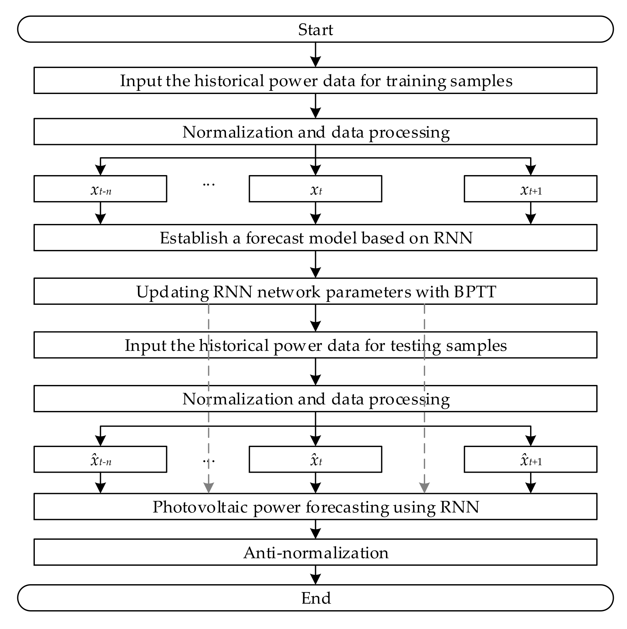
3.3. Forecasting Model Based on RNN

Due to the chaotic nature of the weather conditions, the PV output power data always exhibits a high degree of variability and volatility. Therefore, this study proposes a novel point predictor to mitigate the impact of uncertainty on the accuracy of the PV output power prediction. This predictor is based on the RNN network and considers the adjacent days and intra-day power data. The RNN network has multiple steps input, and the current step input of the hidden layer also includes the state of the previous step hidden layer. This means that the short-term memory attributes based on RNN can better mine the potential links in adjacent days and improve the accuracy of the PV power generation prediction.

As shown in Figure 5, the original PV output power data is divided into a training dataset and a testing dataset. The training dataset and testing dataset are normalized and then arranged in several input sequences. A multi-horizon forecasting model based on RNN is established and trained in a back-propagation through time (BPTT) algorithm [31] to predict the PV output power as accurately as possible.

3.4. Forecasting Performance Evaluation

We select the mean absolute error (MAE), root mean square error (RMSE) and mean absolute percentage error (MAPE) as the evaluation criteria [35]. The evaluation criteria are as follows:

$$\mathrm{MAE}=\frac{1}{N}{\displaystyle \sum _{i=1}^N\left|P_i^a-P_i^f\right|}$$

(25)

$$\mathrm{RMSE}=\sqrt{\frac{1}{N}{\displaystyle \sum _{i=1}^N{\left(P_i^a-P_i^f\right)}^2}}$$

(26)

$$\left\{\begin{array}{l}\mathrm{MAPE}=\frac{1}{N}{\displaystyle \sum _{i=1}^N\frac{\left|P_i^a-P_i^f\right|}{P_{mean}}\times 100\%}\\ P_{mean}=\frac{1}{N}{\displaystyle \sum _{i=1}^N{P}_i^a}\end{array}\right.$$

(27)

where N is the number of test data, P_i^a is the measured power, P_i^f is the predicted power, and P_mean is the average of the total measured power. The MAE and RMSE indexes are used to measure the prediction accuracy, and MAPE is used to measure the degree of deviation between the predicted value and real value. It should be noted that the forecasting method has a high precision when the performance criteria are small.

4. Case Study and Discussions

The main characteristics for the output power of the PV systems are randomness and intermittency. These characteristics can lead to unexpected fluctuations in the voltages and PV power for the PV systems and can cause many problems in power systems, such as power quality, generation control, and storage devices protection. In essence, it is necessary to accurately predict PV power generation to ensure the safe operation and economic integration of the power system [35]. In this paper, the historical solar-PV power data used are collected by Elia, Belgium’s electricity transmission system operator, and the freely downloaded website can be found in the literature [32]. The Flanders photovoltaic power plant has a rated capacity of 2140 MW. The photovoltaic power station transmits electric energy to the common coupling point of the AC grid through DC-DC-AC technology. The active power flow meter is used to measure the active power in real time. Among the collected data, the maximum PV power is 2140 MW and the minimum PV power is 0 MW. The measurement error of the power flow meter is within 0.5%. The measurement error is generally small when compared to the forecasting error. Therefore, the measurement error of PV power plants is generally not considered in this paper, just like other PV power forecasting articles.

Flanders, Belgium is located at 50°51′ north latitude and 4°21′ east longitude, in a temperate maritime climate, and the major features of the year are mild and humid, over the four seasons. Hence, we select four cases from the Flanders Belgium station for a predictive and performance evaluation. The PV power used in this paper are shown in Figure 6, which presents the PV power in Flanders, Belgium for one year. The data cover the period from January 2015 to December 2015 with a 15-minues resolution. The PV power data used in case 1 is from June 30, 2015 to July 31, 2015, and the power data covering the period from December 31, 2015 to January 31, 2016 are adapted to case 2. Similarly, the PV power data used in case 3 and case 4 are from March 31, 2015 to April 30, 2015 and from September 30, 2015 to October 31, 2015, respectively. For each case, the PV power dataset is divided into a training dataset and a testing dataset, which are the data from the 1st to 25th and the rest data, respectively. The training dataset is applied to train the RNN network and extract the nonlinear features hidden in the PV power data, and the testing dataset is used to evaluate the prediction performance of the proposed method. In each case, the predictive model is adapted to each time period through independent training and testing. In order to comprehensively evaluate the forecasting performance of PV power with a multi-time resolution, six forecasting horizons from 15 ahead up to 90 min are presented in this section. In the simulation, Persistence [36], RBF [26], BPNN [24], SVM [25] and LSTM [30] are chosen as benchmark methods to illustrate the improvement of the proposed forecasting model in terms of the forecasting quality.

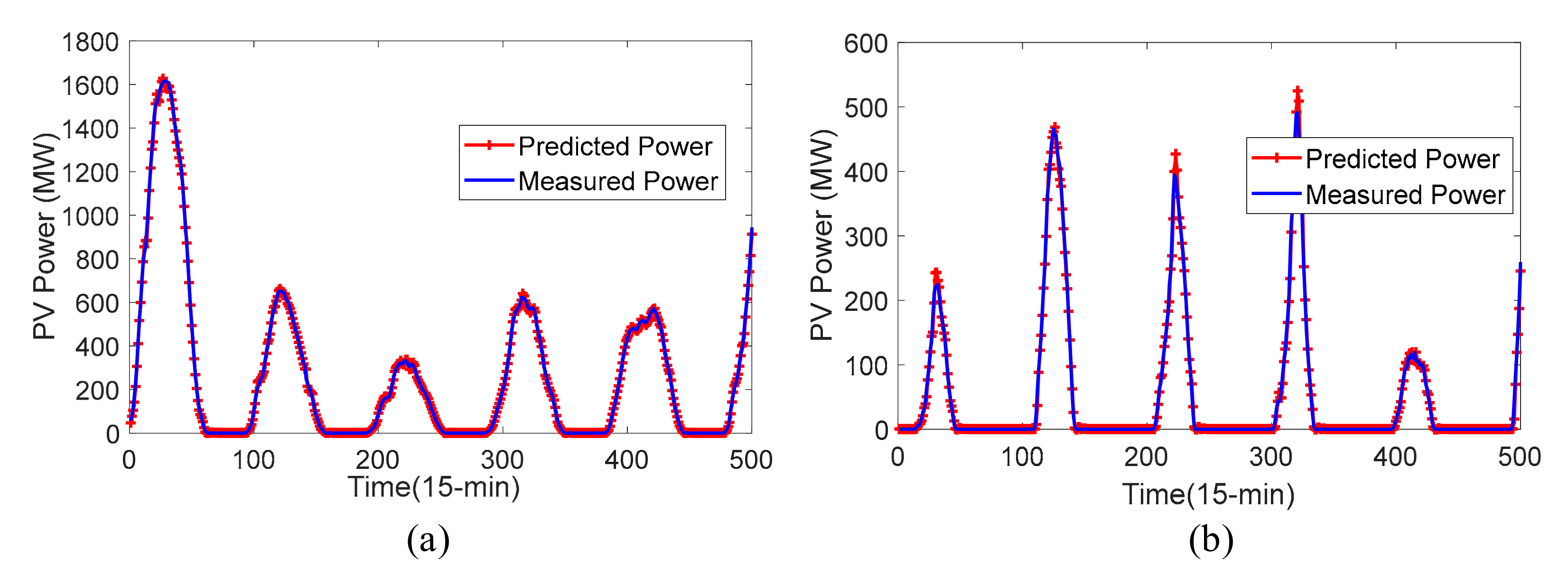
4.1. 15-Min Ahead Forecasting Results

For the 15-min ahead forecasting, the PV power forecasting results of the proposed method in case 1 and case 2 are shown in Figure 7a,b. In the plots, the predicted power curve and measured power curve are a red line and a blue line, respectively. Figure 7a shows the forecasting results of case 1 (Summer) in 15-min-ahead, and it can be seen from the figure that the PV has a higher output power, and the curve will be relatively smoother compared with Figure 7b. As shown in Figure 7b, the output power of case 2 (Winter) is lower than case 1, while the variation amplitude of the power data is larger than case 1. From the curves of Figure 7, we observe that the PV station has a larger and smoother output power curve when the ambient air temperature and solar radiation are high. This is because, at the Flanders Belgium station, the solar temperature and radiation are much stronger in summer than in winter.

The 15-min ahead prediction results of case 1, case 2, case 3 and case 4 obtained from Persistence, RBF, BPNN, SVM, LSTM and the proposed method are presented in

Table 1. Performance evaluation for the 15-min ahead forecasting.

Case	Error	Persistence	RBF	BPNN	SVM	LSTM	Proposed Method
case 1	MAE	17.16	13.47	7.86	9.98	10.96	5.22
	RMSE	27.85	18.31	11.52	13.02	16.11	8.35
	MAPE	6.37%	5.01%	2.92%	3.71%	4.07%	1.94%
case 2	MAE	7.34	7.24	5.36	5.85	4.35	3.44
	RMSE	15.41	12.54	10.18	8.56	8.70	7.35
	MAPE	13.59%	13.39%	9.40%	10.82%	8.04%	6.36%
case 3	MAE	30.10	18.26	9.30	10.97	12.05	6.58
	RMSE	45.34	27.35	14.25	14.46	19.82	10.95
	MAPE	7.07%	4.29%	2.18%	2.58%	2.83	1.54%
case 4	MAE	15.80	9.85	6.52	7.60	6.72	4.17
	RMSE	29.36	15.45	10.20	9.88	11.36	6.97
	MAPE	8.64%	5.39%	3.57%	4.15%	3.67%	2.28%
Average	MAE	17.60	12.21	7.26	8.60	8.52	4.85
	RMSE	29.49	18.41	11.54	11.48	13.99	8.40
	MAPE	8.92%	7.02%	4.52%	5.31%	4.65%	3.03%

. In each case, the predictive model is adapted to each time period through independent training and testing. The best results from the different performance evaluation criteria are highlighted. From the MAE, RMSE and MAPE indexes, the proposed method is superior to the other benchmark methods in all cases. Compared to Persistence, RBF, BPNN, SVM and LSTM, the MAE index has been averagely improved by 72.43%, 60.25%, 33.15%, 43.56% and 43.07%, respectively. Similarly, the RMSE has been evenly improved by 71.51%, 54.37%, 27.17%, 26.78% and 39.96%, respectively, while the MAPE has been improved by 66%, 56.80%, 32.88%, 42.94% and 34.84%, respectively. Meanwhile, both the MAE and RMSE indexes of case 2 are smaller than for the other cases, and the MAPE index is larger than the rest of the cases. This is due to the fact that the PV output powers in July 2015, April 2015 and October 2015 are more stable and more moderate than that in January 2016. The performance evaluation indexes of case 1 and case 2 in Table 1 can be validated from Figure 7.

4.2. 30-Min Ahead Forecasting Results

For the 30-min ahead forecasting, the performance indexes of different methods are shown in

Table 2. Performance evaluation for the 30-min ahead forecasting.

Case	Error	Persistence	RBF	BPNN	SVM	LSTM	Proposed Method
case 1	MAE	34.35	21.46	21.03	20.06	17.81	11.90
	RMSE	55.61	29.27	28.73	26.13	26.50	18.28
	MAPE	12.67%	7.91%	7.76%	7.40%	6.57%	4.39%
case 2	MAE	14.63	12.61	9.56	12.17	7.51	6.87
	RMSE	30.16	21.56	19.34	16.99	15.75	14.27
	MAPE	26.75%	23.06%	17.49%	22.25%	13.73%	12.56%
case 3	MAE	60.09	30.04	22.65	22.67	18.50	13.89
	RMSE	90.15	44.83	33.56	29.49	30.34	22.96
	MAPE	14.04%	7.02%	5.29%	5.29%	4.32%	3.24%
case 4	MAE	31.52	16.80	16.71	16.22	11.66	9.36
	RMSE	58.31	26.25	25.26	20.62	20.11	15.29
	MAPE	17.21%	9.17%	9.12%	8.85%	6.36%	5.11%
Average	MAE	35.15	20.23	17.49	17.78	13.87	10.51
	RMSE	58.56	30.48	26.72	23.30	23.18	17.70
	MAPE	17.67%	11.79%	9.91%	10.95%	7.74%	6.33%

. In the table, the proposed method generates the least MAE, RMSE and MAPE errors out of all four cases, which further reveals the effectiveness of the proposed model. From the average indexes, the LSTM performs better than SVM, BPNN, RBF and Persistence. Moreover, the proposed method has obvious advantages over other benchmarks. It clearly shows the improvement of the proposed method over the benchmark methods in terms of prediction performance in 30-min ahead. Generally speaking, the proposed method performs the best, followed by LSTM, SVM, BPNN, RBF and Persistence. The high precision results mainly result from the RNN architecture, which provides an effective way to mine the weather features in the adjacent days. Therefore, the high-level non-linear, non-stationary characteristics exhibited in the PV power dataset can be better extracted.

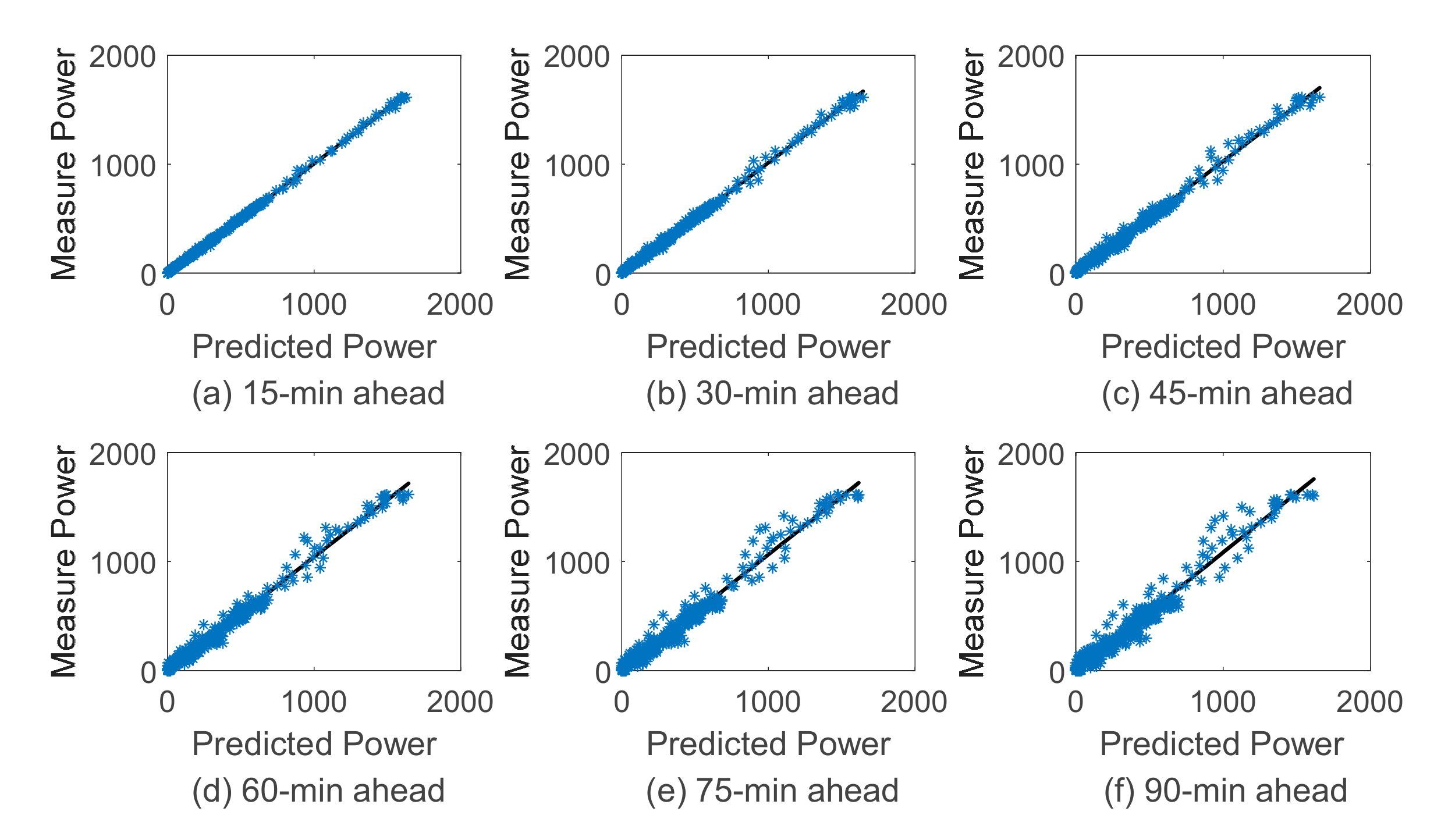
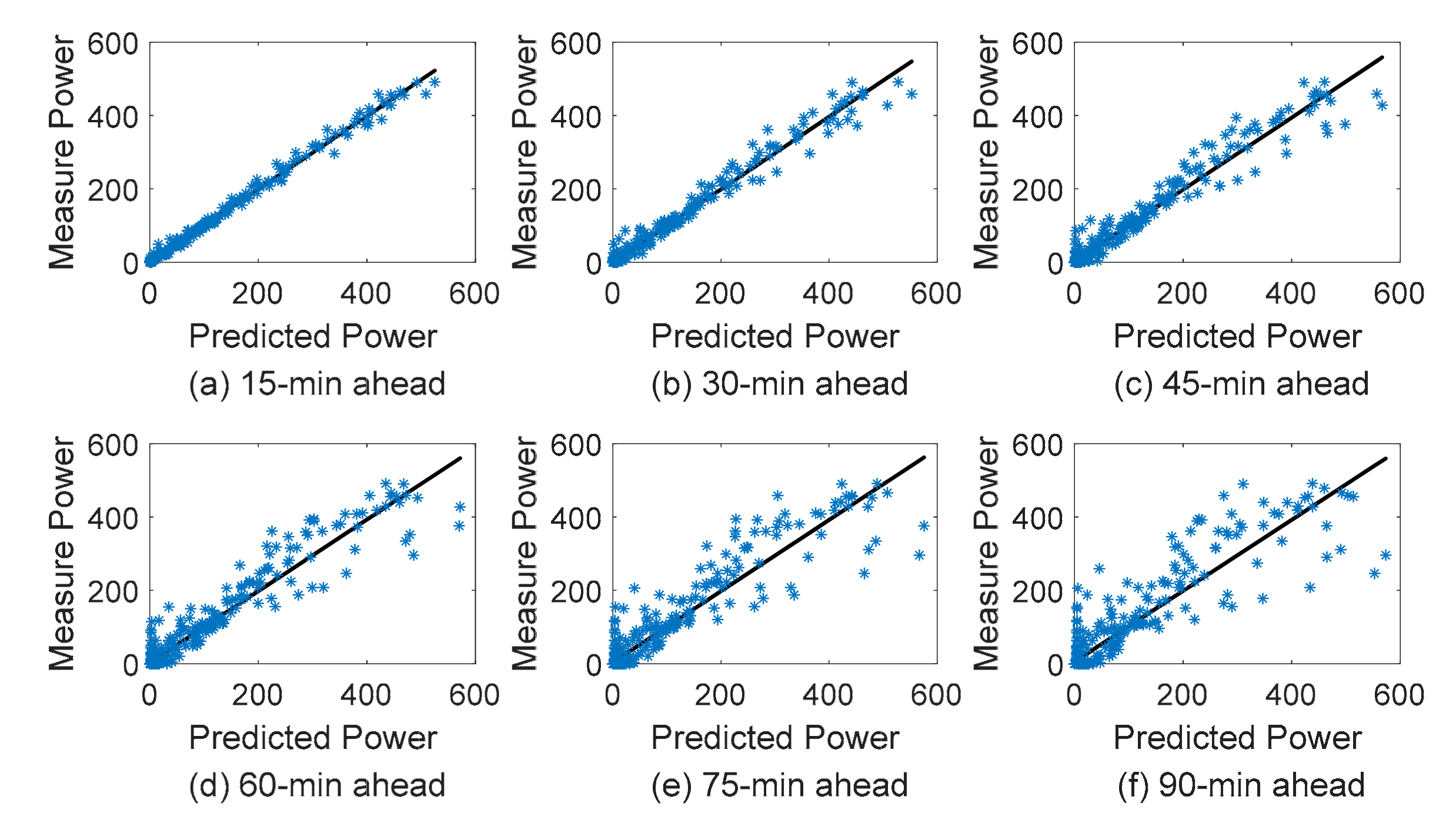
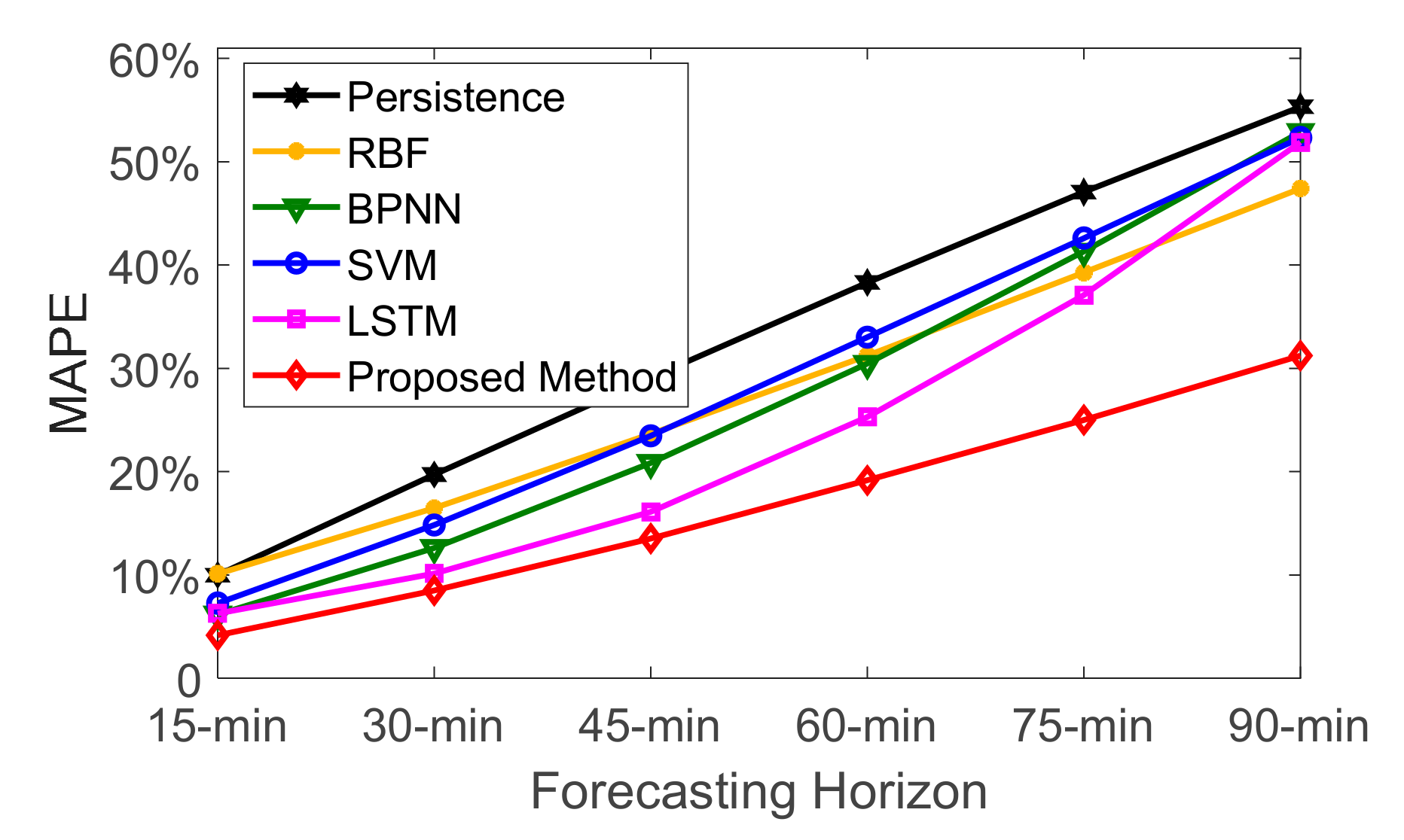
4.3. The Forecasting Results for Multi-step Ahead

To fully verify the feasibility and robustness of the proposed method, simulation experiments are performed under different forecasting horizons. The multi-step ahead forecasting linear regression results (predicted power and measured power) of the proposed method in case 1 and case 2 are shown in Figure 8 and Figure 9. The forecasting horizons are 15-min, 30-min, 45-min, 60-min, 75-min and 90-min, respectively, corresponding to Figure 8a–f and Figure 9a–f. For example, in Figure 8a, the black solid line is the linear regression curve, and the abscissa and ordinate values are the predicted power and measured power, respectively. Meanwhile, the measured power and the predicted power are represented by blue points. As shown in Figure 8, the deviation of the predicted power value from the measured power value increases in case 1 as the forecasting horizon increases. Similarly, the deviation of case 2 increases as the forecasting horizon increases in Figure 9. From the figures, when the prediction step is larger than 60 min, it can be seen that the linear regression results will have a large regression error. Compared to case 1, the forecasting results of case 2 have a significant degradation because of a poor solar radiation stability and low temperature. In terms of the season of the two cases, case 2 belongs to winter with a short illumination time and unstable temperature change. Therefore, the deviation of the multi-steps ahead forecasting results in case 1 is better than in case 2.

In

Table 3. The coefficient of determination R².

Case	Coefficient	15-min	30-min	45-min	60-min	75-min	90-min
case 1	R2	0.9994	0.9975	0.9938	0.9881	0.9800	0.9699
case 2	R2	0.9954	0.9828	0.9619	0.9296	0.8864	0.8359

, we calculate the R² (coefficient of determination) [37] in both case 1 and case 2. The R² is a measure of how the regression line represents the data, and a forecasting model is more efficient when R² is close to 1. From the table, the proposed model exhibits the values of R² (0.9699–0.9994) in case 1, and R² (0.8359–0.9954) in case 2. The results show that our proposed model has a good efficiency in a multi-step prediction. Furthermore, the values of R² deteriorate when the forecasting horizon increases. This implies that the efficiency of the proposed model can be affected by the forecasting horizon. Remarkably, the coefficient of determination in case 2 is worse than in case 1. This shows that the efficiency of the proposed model can also be affected by the seasons in Flanders. This is understandable because the weather environments in case 2 are relatively more chaotic and thus more unpredictable.

In Figure 10, we plot the MAPE curves in different forecasting horizons, where the performance metric value is the average of case 1 and case 2. In addition, Persistence, RBF, BPNN, SVM and LSTM are selected as the reference bases for the proposed method. It can be seen from the figures that the MAPE index increases approximately linearly to the increase of the forecasting horizon; that is, the performance of the prediction model significantly decreases with the increase of the forecasting horizon. This is due to the higher uncertainty and randomness exhibited in the PV power sequences. The BPNN methods have a good forecasting performance in 15-min and 30-min ahead, but could not maintain a good prediction performance in a multi-step prediction due to the inherent limitations of the shallow network. The MAPE index of LSTM increased rapidly with the increase of the forecasting horizon, and the forecasting performances of LSTM in 60, 75 and 90-min are worse than our proposed model. Meanwhile, compared with RBF, BPNN, SVM and LSTM, the proposed method has a significant advantage in the forecasting horizon from 15-min ahead to 90-min ahead. In particular, the proposed method still has a lower prediction error within the 90-min ahead forecasting horizon, with the average MAPE being 31.33%. From the results, it is clear that the MAPE index obtained from the proposed method is significantly better than the benchmarks in all of the prediction horizons, which confirms the high efficiency and performance of the proposed model in solving short-term PV forecasting problems.

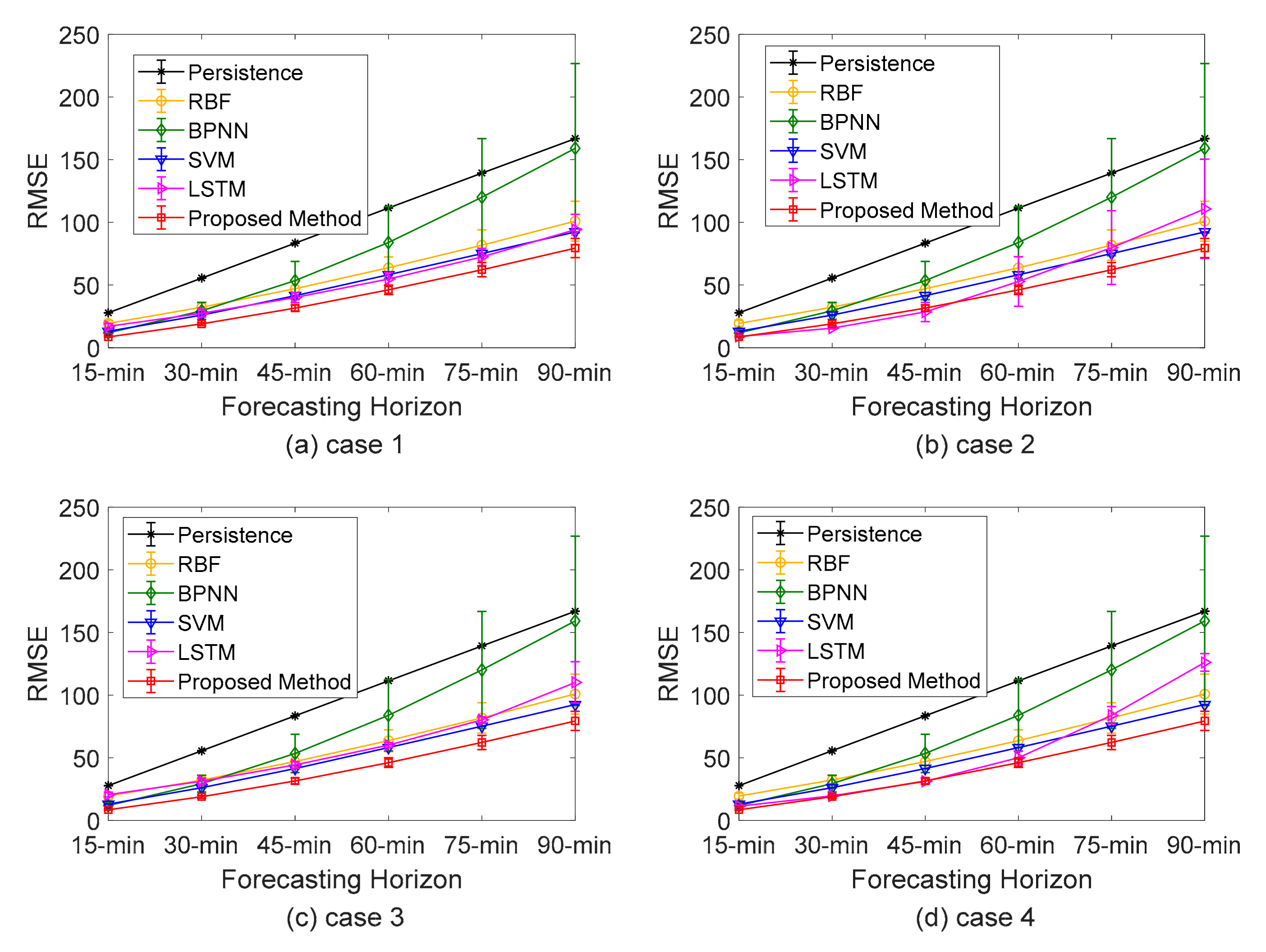
4.4. The Stability and Robustness of Forecasting Model

In this subsection, several simulations of the forecasting model are performed to ensure that the proposed method can provide stable and reliable prediction results. These methods have been run 25 times independently with different forecasting horizons. Figure 11 presents the related error bars of RMSE in case1, case 2, case 3 and case 4. The RMSE in the four cases obtained from the proposed method remains a low error over the forecasting horizons because the recurrent architecture and memory units are determined, and the adjacent power data in each forecasting process is utilized. As can be seen from the figure, the prediction error of the persistence forecasting model is large. The RMSE index of BPNN method fluctuates wildly, indicating that the prediction performance is not stable enough, which is not desirable in a practical application. Although the prediction performance of the RBF and SVM methods are relatively stable, their prediction accuracy still needs to be improved. The RMSE index of LSTM increases with the increase of the forecasting horizon, and its performance deteriorates rapidly when the forecasting horizon is large. Obviously, the averaged RMSE of the proposed method is the best among the benchmarks. In addition, the result of LSTM outperforms the RBF, BPNN and SVM in 15, 30, 45 and 60-min, which is consistent with the recurrent architecture in [30]. Meanwhile, the complex structure of LSTM and the accumulation of errors in the multi-step prediction will lead to a large prediction error in 75 and 90-min. We can see that the prediction performance of the proposed method is more stable than RBF and BPNN, and that the error is smaller than Persistence, SVM and LSTM. These results show that our method can provide a reliable prediction result for the PV power generation prediction. Hence, from the numerical results, we can easily conclude that the proposed method exhibits the most desirable performance for PV power forecasting.

5. Conclusions

In this paper, we have proposed a new RNN-based short-term method for forecasting PV power. Unlike traditional forecasting methods, we feed the PV power of adjacent days to the RNN model, where the similarity and correlation have been verified with the real power data in Flanders, Belgium. The proposed forecasting model with a recurrent architecture and memory units can effectively learn the power changes and features in both the inter-day and intra-day PV power. Then, the proposed method has been comprehensively compared with the LSTM, SVM, RBF, BPNN and Persistence methods. Some results demonstrate that the average MAPE, RMSE and MAE of the proposed method outperform the benchmarks in the 15-min and 30-min forecasting horizons. Meanwhile, the proposed method also has a good prediction performance in different cases and forecasting horizons. Therefore, the proposed method can provide stable and reliable power forecasting for the actual PV power plants. Furthermore, the proposed method can be used to promote the future application of solar energy.

References

1. Sahu, B.K. A study on global solar PV energy developments and policies with special focus on the top ten solar PV power producing countries. Renew. Sustain. Energy Rev. 2015, 43, 621–634. [Google Scholar] [CrossRef]
2. Sobri, S.; Koohi-Kamali, S.; Rahim, N.A. Solar photovoltaic generation forecasting methods: A review. Energy Convers. Manag. 2018, 156, 459–497. [Google Scholar] [CrossRef]
3. Antonanzas, J.; Osorio, N.; Escobar, R.; Urraca, R.; Martinez-De-Pison, F.J.; Antonanzas-Torres, F. Review of photovoltaic power forecasting. Sol. Energy 2016, 136, 78–111. [Google Scholar] [CrossRef]
4. Riffonneau, Y.; Bacha, S.; Barruel, F.; Ploix, S. Optimal power flow management for grid connected PV systems with batteries. IEEE Trans. Sustain. Energy 2011, 2, 309–320. [Google Scholar] [CrossRef]
5. Mohamed, A.; Salehi, V.; Ma, T.; Mohammed, O. Real-time energy management algorithm for plug-in hybrid electric vehicle charging parks involving sustainable energy. IEEE Trans. Sustain. Energy 2014, 5, 577–586. [Google Scholar] [CrossRef]
6. Chen, C.; Duan, S.; Cai, T.; Liu, B.; Hu, G. Smart energy management system for optimal microgrid economic operation. IET Renew. Power Gener. 2011, 5, 258–267. [Google Scholar] [CrossRef]
7. Chen, X.; Du, Y.; Wen, H. Forecasting based power ramp-rate control for pv systems without energy storage. In Proceedings of the 2017 IEEE 3rd International Future Energy Electronics Conference and ECCE Asia (IFEEC 2017-ECCE Asia), Kaohsiung, Taiwan, 27 July 2017; pp. 733–738. [Google Scholar]
8. Litjens, G.; Worrell, E.; van Sark, W. Assessment of forecasting methods on performance of photovoltaic-battery systems. Appl. Energy 2018, 221, 358–373. [Google Scholar] [CrossRef]
9. Kikusato, H.; Mori, K.; Yoshizawa, S.; Fujimoto, Y.; Asano, H.; Hayashi, Y.; Kawashima, A.; Inagaki, S.; Suzuki, T. Electric vehicle charge-discharge management for utilization of photovoltaic by coordination between home and grid energy management systems. IEEE Trans. Smart Grid 2018, 10, 3186–3197. [Google Scholar] [CrossRef]
10. Ming, M.; Wang, R.; Zha, Y.; Zhang, T. Multi-objective optimization of hybrid renewable energy system using an enhanced multi-objective evolutionary algorithm. Energies 2017, 10, 674. [Google Scholar] [CrossRef]
11. Wang, G.; Zhang, X.; Wang, H.; Peng, J.-C.; Jiang, H.; Liu, Y.; Wu, C.; Xu, Z.; Liu, W. Robust Planning of Electric Vehicle Charging Facilities with an Advanced Evaluation Method. IEEE Trans. Ind. Inform. 2018, 14, 866–876. [Google Scholar] [CrossRef]
12. Giorgi, M.G.D.; Congedo, P.M.; Malvoni, M.; Laforgia, D. Error analysis of hybrid photovoltaic power forecasting models: A case study of mediterranean climate. Energy Convers. Manag. 2015, 100, 117–130. [Google Scholar] [CrossRef]
13. Inman, R.H.; Pedro, H.T.C.; Coimbra, C.F.M. Solar forecasting methods for renewable energy integration. Prog. Energy Combust. Sci. 2013, 39, 535–576. [Google Scholar] [CrossRef]
14. Xu, R. The restriction research for urban area building integrated grid-connected PV power generation potential. Energy 2016, 113, 124–143. [Google Scholar]
15. Wang, F.; Mi, Z.; Su, S.; Zhao, H. Short-term solar irradiance forecasting model based on artificial neural network using statistical feature parameters. Energies 2012, 5, 1355–1370. [Google Scholar] [CrossRef]
16. Wang, H.Z.; Wang, G.B.; Li, G.Q.; Peng, J.C.; Liu, Y.T.; Yan, J. Deep belief network based deterministic and probabilistic wind speed forecasting approach. Appl. Energy 2016, 182, 80–93. [Google Scholar] [CrossRef]
17. Hong, Y.-Y.; Yu, T.-H.; Liu, C.-Y. Hour-ahead wind speed and power forecasting using empirical mode decomposition. Energies 2013, 6, 6137–6152. [Google Scholar] [CrossRef]
18. Gotleyb, D.; Sciuto, G.L.; Napoli, C.; Shikler, R.; Tramontana, E.; Woźniak, M. Characterisation and modeling of organic solar cells by using radial basis neural networks. In Proceedings of the International Conference on Artificial Intelligence and Soft Computing, Zakopane, Poland, 12–16 June 2016; Springer: Berlin, Germany; pp. 91–103. [Google Scholar]
19. Połap, D.; Woźniak, M.; Wei, W.; Damaševičius, R. Multi-threaded learning control mechanism for neural networks. Fut. Gen. Comput. Syst. 2018, 87, 16–34. [Google Scholar]
20. Aderemi, O.; Misra, S.; Ahuja, R. Energy Consumption Forecast Using Demographic Data Approach with Canaanland as Case Study. In Proceedings of the International Conference on Next Generation Computing Technologies, Dehradun, India, 30–31 October 2017; pp. 641–652. [Google Scholar]
21. Beritelli, F.; Capizzi, G.; Sciuto, G.L.; Scaglione, F.; Połap, D.; Woźniak, M. A neural network pattern recognition approach to automatic rainfall classification by using signal strength in LTE/4G networks. In Proceedings of the International Joint Conference on Rough Sets, Olsztyn, Poland, 3–7 July 2017; Springer: Berlin, Germany; pp. 505–512. [Google Scholar]
22. Sciuto, G.L.; Capizzi, G.; Caramagna, A.; Famoso, F.; Lanzafame, R.; Woźniak, M. Failure Classification in High Concentration Photovoltaic System (HCPV) by using Probabilistic Neural Networks. Int. J. Appl. Eng. Res. 2017, 12, 16039–16046. [Google Scholar]
23. Pedro, H.T.C.; Coimbra, C.F.M. Assessment of forecasting techniques for solar power production with no exogenous inputs. Sol. Energy 2012, 86, 2017–2028. [Google Scholar] [CrossRef]
24. Zhu, H.; Lian, W.; Lu, L.; Dai, S.; Hu, Y. An improved forecasting method for photovoltaic power based on adaptive BP neural network with a scrolling time window. Energies 2017, 10, 1542. [Google Scholar] [CrossRef]
25. Shi, J.; Lee, W.J.; Liu, Y.; Yang, Y.; Wang, P. Forecasting Power Output of Photovoltaic Systems Based on Weather Classification and Support Vector Machines. IEEE Trans. Ind. Appl. 2015, 48, 1064–1069. [Google Scholar] [CrossRef]
26. Wu, C.; Mohsenian-Rad, H.; Huang, J. Vehicle-to-aggregator interaction game. IEEE Trans. Smart Grid 2011, 3, 434–442. [Google Scholar] [CrossRef]
27. Ugurlu, U.; Oksuz, I.; Tas, O. Electricity price forecasting using recurrent neural networks. Energies 2018, 11, 1255. [Google Scholar] [CrossRef]
28. Yona, A.; Senjyu, T.; Funabashi, T. Application of Recurrent Neural Network to Short-Term-Ahead Generating Power Forecasting for Photovoltaic System. In Proceedings of the Power Engineering Society General Meeting, Tampa, FL, USA, 24–28 June 2007; pp. 1–6. [Google Scholar]
29. Yadav, A.P.; Kumar, A.; Behera, L. RNN Based Solar Radiation Forecasting Using Adaptive Learning Rate. In Proceedings of the International Conference on Swarm Evolutionary and Memetic Computing, Chennai, India, 19–21 December 2013; Springer: Berlin, Germany, 2013; pp. 442–452. [Google Scholar]
30. Abdel-Nasser, M.; Mahmoud, K. Accurate photovoltaic power forecasting models using deep LSTM-RNN. Neural Comput. Appl. 2017, 1–14. [Google Scholar] [CrossRef]
31. Goodfellow, I.; Bengio, Y.; Courville, A. Deep Learning; The MIT Press: London, UK, 2016. [Google Scholar]
32. Elia, Belgium’s Electricity Transmission System Operator. Available online: http://www.elia.be/en/grid-data/power-generation/Solar-power-generation-data/Graph (accessed on 31 December 2014).
33. He, Y.-J.; Zhu, Y.-C.; Gu, J.-C.; Yin, C.-Q. Similar day selecting based neural network model and its application in short-term load forecasting. In Proceedings of the 2005 International Conference on Machine Learning and Cybernetics, Guangzhou, China, 18–21 August 2005; pp. 4760–4763. [Google Scholar]
34. Sun, X.; Luh, P.B.; Cheung, K.W.; Guan, W.; Michel, L.D.; Venkata, S.; Miller, M.T. An efficient approach to short-term load forecasting at the distribution level. IEEE Trans. Power Syst. 2016, 31, 2526–2537. [Google Scholar] [CrossRef]
35. Wang, H.; Yi, H.; Peng, J.; Wang, G.; Liu, Y.; Jiang, H.; Liu, W. Deterministic and probabilistic forecasting of photovoltaic power based on deep convolutional neural network. Energy Convers. Manag. 2017, 153, 409–422. [Google Scholar] [CrossRef]
36. Yang, C.; Thatte, A.A.; Xie, L. Multitime-scale data-driven spatio-temporal forecast of photovoltaic generation. IEEE Trans. Sustain. Energy 2014, 6, 104–112. [Google Scholar] [CrossRef]
37. Shah, A.S.B.M.; Yokoyama, H.; Kakimoto, N. High-precision forecasting model of solar irradiance based on grid point value data analysis for an efficient photovoltaic system. IEEE Trans. Sustain. Energy 2015, 6, 474–481. [Google Scholar] [CrossRef]
Figure 1. The structure of recurrent neural network (RNN).
Energies 12 02538 g001
Figure 2. The PV power generation curves of adjacent days in Flanders, Belgium.
Energies 12 02538 g002
Figure 3. The similarity degree in adjacent days for k-day intervals.
Energies 12 02538 g003
Figure 4. The inputs of RNN for the PV power forecasting.
Energies 12 02538 g004
Figure 5. The flowchart for the PV generation power forecasting.
Energies 12 02538 g005
Figure 6. The PV power curves in Flanders, Belgium.
Energies 12 02538 g006
Figure 7. 15-min ahead of the PV power forecasting results. (a) Case 1; (b) Case 2.
Energies 12 02538 g007
Figure 8. (af). The results of the linear regression for the predicted and measured power in case 1.
Energies 12 02538 g008
Figure 9. (af). The results of the linear regression for the predicted and measured power in case 2.
Energies 12 02538 g009
Figure 10. Average MAPE statistics for case 1 and case 2 in terms of various forecasting horizons.
Energies 12 02538 g010
Figure 11. RMSE statistics in terms of various forecasting horizons.
Energies 12 02538 g011