Research on the Energy-Saving Strategy of Path Planning for Electric Vehicles Considering Traffic Information

Abstract

Battery-powered electric vehicles (EVs) have a limited on-board energy storage and present the problem of driving mileage anxiety. Moreover, battery energy storage density cannot be effectively improved in a short time, which is a technical bottleneck of EVs. By considering the impact of traffic information on energy consumption forecasting, an energy-saving path planning method for EVs that takes traffic information into account is proposed. The modeling process of the EV model and the construction process of the traffic simulation model are expounded. In addition, the long-term, short-term memory neural network (LSTM) model is selected to predict the energy consumption of EVs, and the sequence to sequence technology is used in the model to integrate the driving condition data of EVs with traffic information. In order to apply the predicted energy consumption to travel guidance, a road planning method with the optimal coupling of energy consumption and distance is proposed. The experimental results show that the energy-based economic path uses 9.9% lower energy consumption and 40.2% shorter travel time than the distance-based path, and a 1.5% lower energy consumption and 18.6% longer travel time than the time-based path.

1. Introduction

The development of electric vehicles (EVs) can effectively solve environmental pollution, improve urban air quality, and alleviate energy shortage pressure [1,2]. However, the drivers are often plagued by EV mileage anxiety, which affects the driving experience due to the limitation of power battery capacity and worrying about the unknown energy consumption on future road segments [3]. The driving range of the remaining energy of the power battery is generally estimated based on the new european driving cycle (NEDC) [4] and the path planning method commonly used in EVs in travel navigation is based on the shortest travel route [5]. The disadvantage of this method is that NEDCs are different from the actual traffic conditions [6] and the occupants cannot know whether the remaining energy is enough to reach the destination. In daily travel, the shortest path may result in wasted energy consumption of EVs due to traffic congestion and, therefore, the travel time will also increase [7,8].

To effectively reduce energy consumption and improve driving range, previous research on the energy management of EVs have investigated nonlinear model predictive control [9], multi-objective optimization [10], RBF-neural network [11], estimation of preceding vehicle future movements [12], global optimization [13], and deep learning [14]; however, the above-mentioned papers neglect the influence of the actual traffic conditions. To solve such problems, a new modal activity framework for vehicle energy/emissions estimation using sparse mobile sensor data is presented in reference [15] and a data-driven model is built to estimate EV energy consumption on each roadway link considering real-world traffic conditions in reference [16]. For the complicated energy system of a plug-in hybrid electric vehicle, a generic framework of an online energy management system that is based on an evolutionary algorithm is proposed and can achieve the best fuel economy improvement, which require less trip information in reference [17]. It is possible to predict future energy consumption based on the vehicle historical states and predict the remaining driving range more accurately based on the future driving conditions under the help of traffic information.

In this paper, based on the information of a traffic network, the driving conditions of EVs are fully considered to accurately predict the energy consumption and the problem of the energy-saving path with optimal coupling of energy consumption and distance is discussed and the solution method is explored with the aim being to effectively alleviate mileage anxiety. Finally, the travel time and travel energy consumption are reasonably reduced, while the accuracy and effectiveness of the method are verified by simulation experiments.

The article structure is arranged in seven sections. Section 2 builds the models of the battery-powered electric car and then verifies the models with experimental data. Section 3 builds the models of the traffic network. Section 4 puts forward an LSTM model to perform the prediction of energy consumption and sequence to sequence technology is used in the model to integrate the driving condition data of EVs with the traffic information based on the models built in Section 2 and Section 3. Section 5 gives a planning strategy for an optimal coupling path between energy consumption and distance. Section 6 performs three kinds of experiments: distance-based, energy-based, and time-based optimal simulations, and provides the results. Section 7 lists the main conclusions.

2. Battery-Powered Electric Vehicle Modeling

In order to accurately obtain the driving energy consumption, a battery-powered EV model is built based on the EU260 electric car. The EV model includes a driver model, driving system model, power battery model, and vehicle dynamics model [18,19,20,21].

2.1. Driver Model

A proportional-integral-derivative controller (PID) is used to model the driver to accurately follow the actual vehicle speed with the desired speed as shown in Equation (1) [19].

$$P_{\mathrm{acc}}=\frac{1}{P_{\mathrm{ed}}}\left(K_{\mathrm{p}}{v}_{\mathrm{e}}+{\alpha }_i{K}_{\mathrm{i}}{\displaystyle {\int }_0^t{v}_{\mathrm{e}}\mathrm{d}t}\right)\times 100\%$$

(1)

$$v_{\mathrm{e}}=v_{\mathrm{pre}}-v_{\mathrm{act}}$$

(2)

$${\alpha }_i=\{\begin{array}{c}0,\begin{array}{cc}& \left|K_{\mathrm{i}}{\displaystyle {\int }_0^t{v}_{\mathrm{e}}\mathrm{d}t}\right|>P_{\mathrm{ed}}\end{array}\\ 1,\begin{array}{cc}& \left|K_{\mathrm{i}}{\displaystyle {\int }_0^t{v}_{\mathrm{e}}\mathrm{d}t}\right|\le P_{\mathrm{ed}}\end{array}\end{array}$$

(3)

where $v_{\mathrm{pre}}$ is the expected speed, $v_{\mathrm{act}}$ is the actual speed, $v_{\mathrm{e}}$ is the difference between the actual speed and the expected speed, ${\alpha }_{\mathrm{i}}$ is the integral anti-saturation parameter of the PID regulator, $K_{\mathrm{p}}$ is the proportional parameter of PID, $K_{\mathrm{i}}$ is the integral parameter of PID, and $P_{\mathrm{acc}}$ is the depth of the accelerator pedal or brake pedal, P_ed is the full-scale depth of the accelerator pedal or brake pedal with the value range of [−100%, 100%]. If $P_{\mathrm{acc}}$ is negative, it means that the EV is braking. If it is positive, it means the EV is speeding up [22,23].

2.2. Driving System Model

The vehicle driving model is built with Equations (4)–(7)

$${\mathrm{F}}_{\mathrm{tra}}=T_{\mathrm{out}}{\eta }_{\mathrm{wheel}}/r$$

(4)

$$T_{\mathrm{out}}=P_{\mathrm{acc}}{T}_{\max }$$

(5)

$$T_{\mathrm{motor}}=T_{\mathrm{out}}/{\eta }_{\mathrm{t}}$$

(6)

$$P_{\mathrm{motor}}=T_{\mathrm{motor}}{\omega }_{\mathrm{motor}}$$

(7)

where $F_{\mathrm{tra}}$ is the driving force of the tire, r is the tire rolling radius of the driving wheel, $T_{\mathrm{out}}$ is the output torque of the motor drive system, ${\eta }_{\mathrm{wheel}}$ is the transmission efficiency between the drive system and the wheel, ${\eta }_{\mathrm{wheel}}=98\%$, and $T_{\max }$ is the maximum torque that the motor drive system can output, the peak power of the driving motor is 100 kW and its maximum torque is 265 Nm. $T_{\mathrm{motor}}$ is the output torque of the driving motor, ${\eta }_{\mathrm{t}}$ is the efficiency of the motor drive system, $P_{\mathrm{motor}}$ is the output power of the driving motor, and ${\omega }_{\mathrm{motor}}$ is the output speed of the driving motor.

2.3. Power Battery Model

The Rint circuit model is selected as the equivalent circuit model of the power battery [20]. The Rint model consists of an ideal voltage source and a resistor [24].

$${\mathrm{P}}_{\mathrm{batt}}=P_{\mathrm{motor}}/{\eta }_{\mathrm{m}}$$

(8)

$$P_{\mathrm{batt}}=U_{\mathrm{oc}}{I}_{\mathrm{L}}-I_{\mathrm{L}}{}^2{R}_0$$

(9)

$$I_{\mathrm{L}}=\frac{U_{o\mathrm{c}}-\sqrt{U_{o\mathrm{c}}{}^2-4R_0{P}_{\mathrm{batt}}}}{2R_0}$$

(10)

$$SO{C}_{\mathrm{t}}=SO{C}_0-\frac{{\displaystyle {\int }_0^t{\eta }_{\mathrm{batt}}{I}_{\mathrm{L}}\mathrm{d}t}}{Q_{\mathrm{b}}}$$

(11)

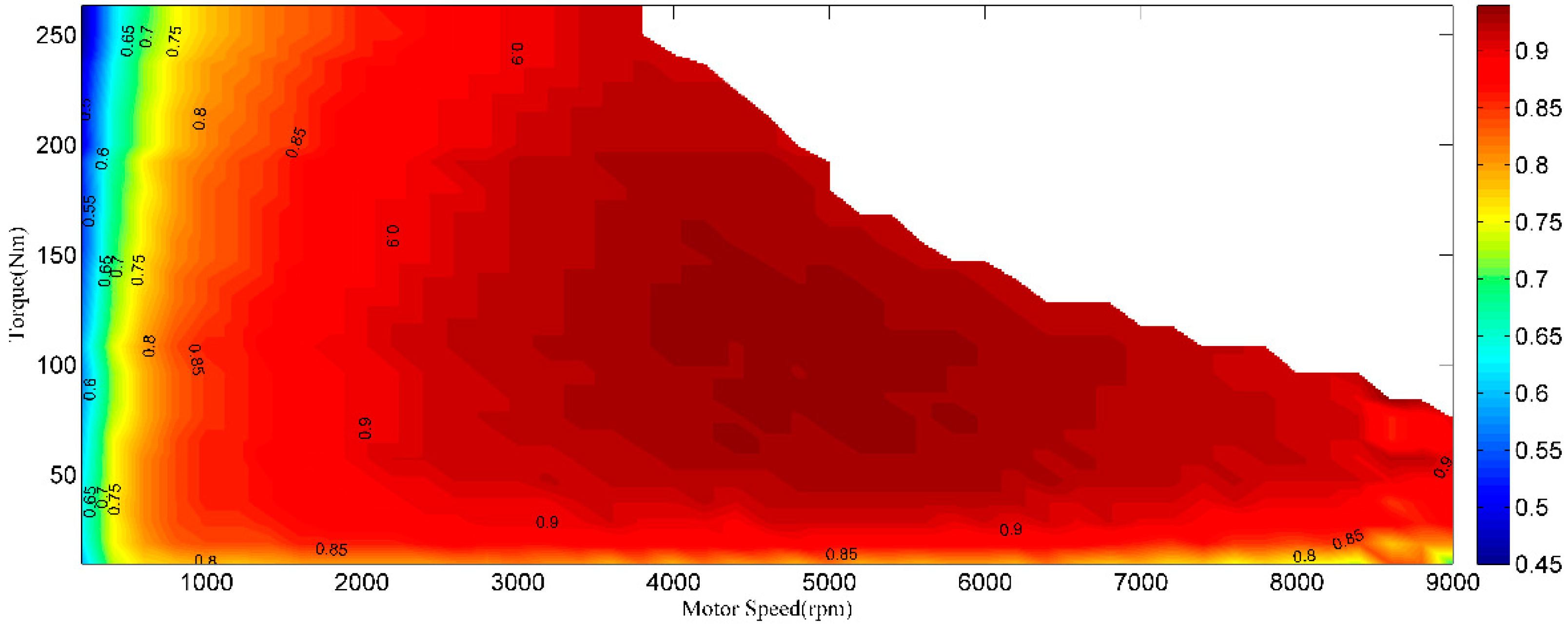
where $P_{\mathrm{batt}}$ is the battery output power, η_m is the efficiency of the driving motor system including motor and motor controller, which can be obtained by the look-up table method based on the efficiency map shown as Figure 1; $U_{\mathrm{oc}}$ is the battery open-circuit voltage, $I_{\mathrm{L}}$ is the battery operating current, $R_0$ is the battery internal resistance, and here $U_{\mathrm{oc}}$ and $R_0$ can be measured with the experimental method [25]. $SO{C}_{\mathrm{t}}$ is the SOC to be solved, $SO{C}_0$ is the initial value of the power battery SOC, $Q_{\mathrm{b}}$ is the total capacity of the power battery, which decreases with the decrease of a battery state of health (SOH) [21], ${\eta }_{\mathrm{batt}}$ is the power battery charge and discharge efficiency.

$${\eta }_{\mathrm{batt}}=\{\begin{array}{l}98\%,I_{\mathrm{L}}<0\\ 100\%,I_{\mathrm{L}}\ge 0\end{array}$$

(12)

When the battery is charging ($I_{\mathrm{L}}<0$), ${\eta }_{\mathrm{batt}}=98\%$, and when the battery in in discharging ($I_L\ge 0$), ${\eta }_{\mathrm{batt}}=100\%$.

The SOC of the power battery can be solved according to the above Equation (10).

2.4. Vehicle Driving Dynamics Model

The vehicle driving dynamics model was built with Equations (13)–(16)

$$F_{\mathrm{tra}}=F_{\mathrm{g}}+F_{\mathrm{r}}+F_{\mathrm{a}}+\delta \mathrm{m}a$$

(13)

$$F_{\mathrm{g}}=mg\sin \theta$$

(14)

$$F_{\mathrm{r}}=mg\cos \theta C_r$$

(15)

$$F_{\mathrm{a}}=\frac{1}{2}{\rho }_a{C}_a{A}_f{v}^2$$

(16)

where $m$ is the total mass of the EV, $\delta$ is the equivalent coefficient of the EV moment inertia, $a$ is the EV acceleration rate, $F_{\mathrm{tra}}$ is the driving force, $F_{\mathrm{g}}$ is the gravity resistance along the road surface, $F_{\mathrm{r}}$ is the rolling resistance, and $F_{\mathrm{a}}$ is the air resistance. $g$ is the gravitational acceleration, $\theta$ is the road gradient, and $C_{\mathrm{r}}$ is the tire rolling resistance coefficient. ${\rho }_{\mathrm{a}}$ is the air density, $C_{\mathrm{a}}$ is the air resistance coefficient, $A_{\mathrm{f}}$ is the windward area of the EV, and $v$ is the EV speed.

2.5. Verification of the Accuracy of the EV Model

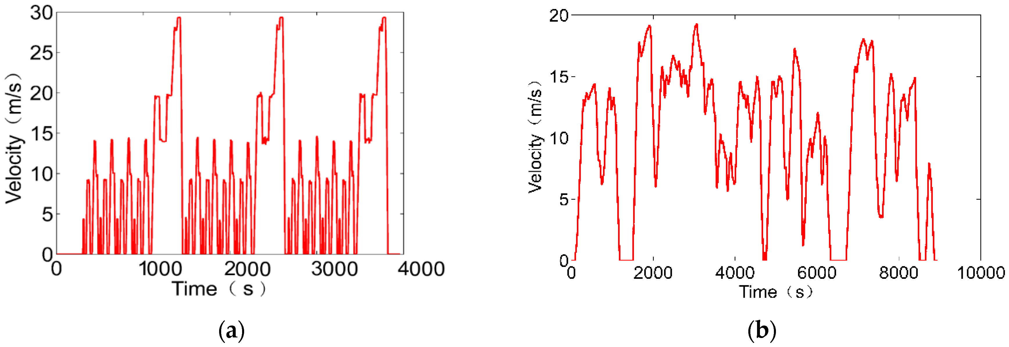
The accuracy of the vehicle model is verified through the energy consumption comparison between the simulation and experiment, the driving cycle input is designed as the 3 continuous NEDC driving cycles on the test bench [26] and an actual road driving cycle as shown in Figure 2a,b.

After the three NEDCs shown in Figure 2a, the real vehicle consumes 11.8% of the total energy and the model consumes 12.1% of the total energy with an error of 0.3% as listed in

Table 1. Comparison of energy consumption between the real vehicle and the model for 3 NEDCs.

Vehicle Type	Driving Condition	Energy Consumption
Real Vehicle	3 NEDCs on test bench	11.8%
Model	3 NEDCs input	12.1%

.

As listed in

Table 2. Comparison of energy consumption between the real vehicle and the model for actual road driving.

Vehicle Type	Driving Condition	Energy Consumption
Real Vehicle	Actual road driving	7.0%
Model	Actual road driving cycle input	7.2%

, after running 8939 s on an actual road as shown in Figure 2b, the real vehicle runs for 18.01 km and consumes 7.0% of the total energy and the model consumes 7.2% of the total energy with an error of 2.8%.

According to the above two conditions, it can be considered that the vehicle model has enough accuracy when calculating energy consumption.

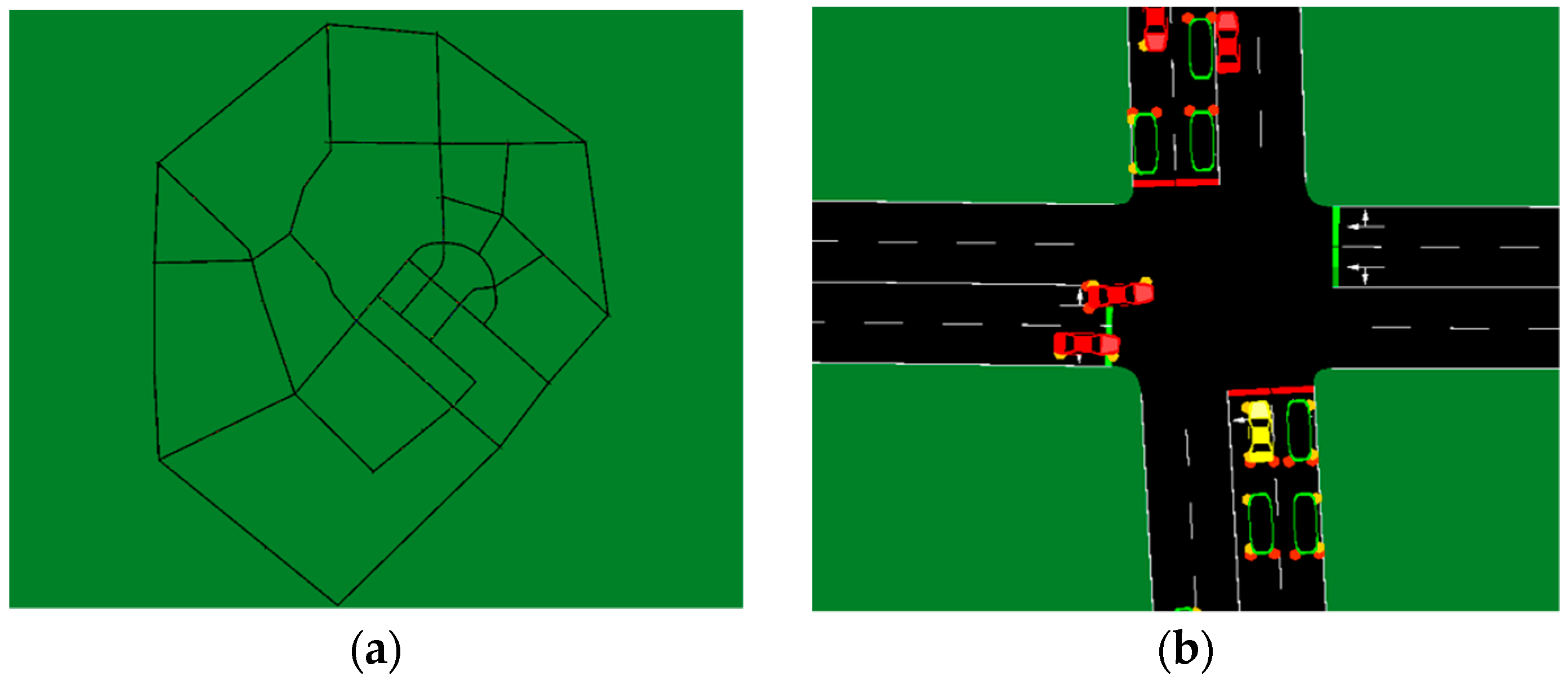
3. Modeling of the Traffic Network

The SUMO (Simulation of Urban Mobility) [27] high-precision urban traffic simulation software is used to simulate the traffic network. The main task is to layout and plan the roads and intersections, then use the actual observation data to design the traffic parameters. Based on the traffic network of the Chaoyang District of Beijing, which is about 4 km long and about 5 km wide, a total of 20 km² regions, the traffic network simulation model is established, as shown in Figure 3.

The traffic network parameters are set according to the observation data as listed in

Table 3. Actual observed traffic data.

Data Observation	Value
Number of roads	3
Observation period	Monday to Friday 16:30–17:30
Average traffic flow	380 vehicles/min
Average traffic density	80 vehicles/km
Average speed	34 km/h

. By continuously adjusting the traffic model parameters manually, the traffic flow data of the traffic model is close to the observed data. Finally, we get the manually set origin-destination matrix (OD Matrix) as listed in Matrix (17); the value (x, y) of the matrix represents vehicles per hour from the starting point x to the end point y. The value of (x, y) is manually adjusted based on the observed data in Table 3.

$$\left[\begin{array}{ccccc}0& 40& \dots & 4& 21\\ 100& 0& \dots & 110& 30\\ \dots & \dots & 0& \dots & \dots \\ 200& 220& \dots & 0& 150\\ 190& 460& \dots & 260& 0\end{array}\right]$$

(17)

According to the proportion of the vehicles on the actual road, the proportion of each type of vehicle is set as

Table 4. The proportion of each vehicle type in the traffic simulation model.

Vehicle Type	Value
Fuel family vehicle	50%
EV	10%
Bus	10%
Taxi	20%
Truck	8%
Cleaning vehicle	2%

. In the traffic model, the vehicle-following model of each type of vehicle is defined according to the vehicle-following model recommended by the SUMO software. Python controls the SUMO run and sets the parameters in the SUMO simulation through the TraCI [28] interface protocol and the traffic data generated by the SUMO simulation can also be accessed in Python for the next step of data processing.

The vehicle model is put into the road network of the traffic simulation model for joint simulation, and the traffic information data and the driving condition data set of EVs are obtained. The data set lays a foundation for the energy consumption prediction model.

4. A Prediction of EV Energy Consumption Integrating Traffic Information and Driving Data

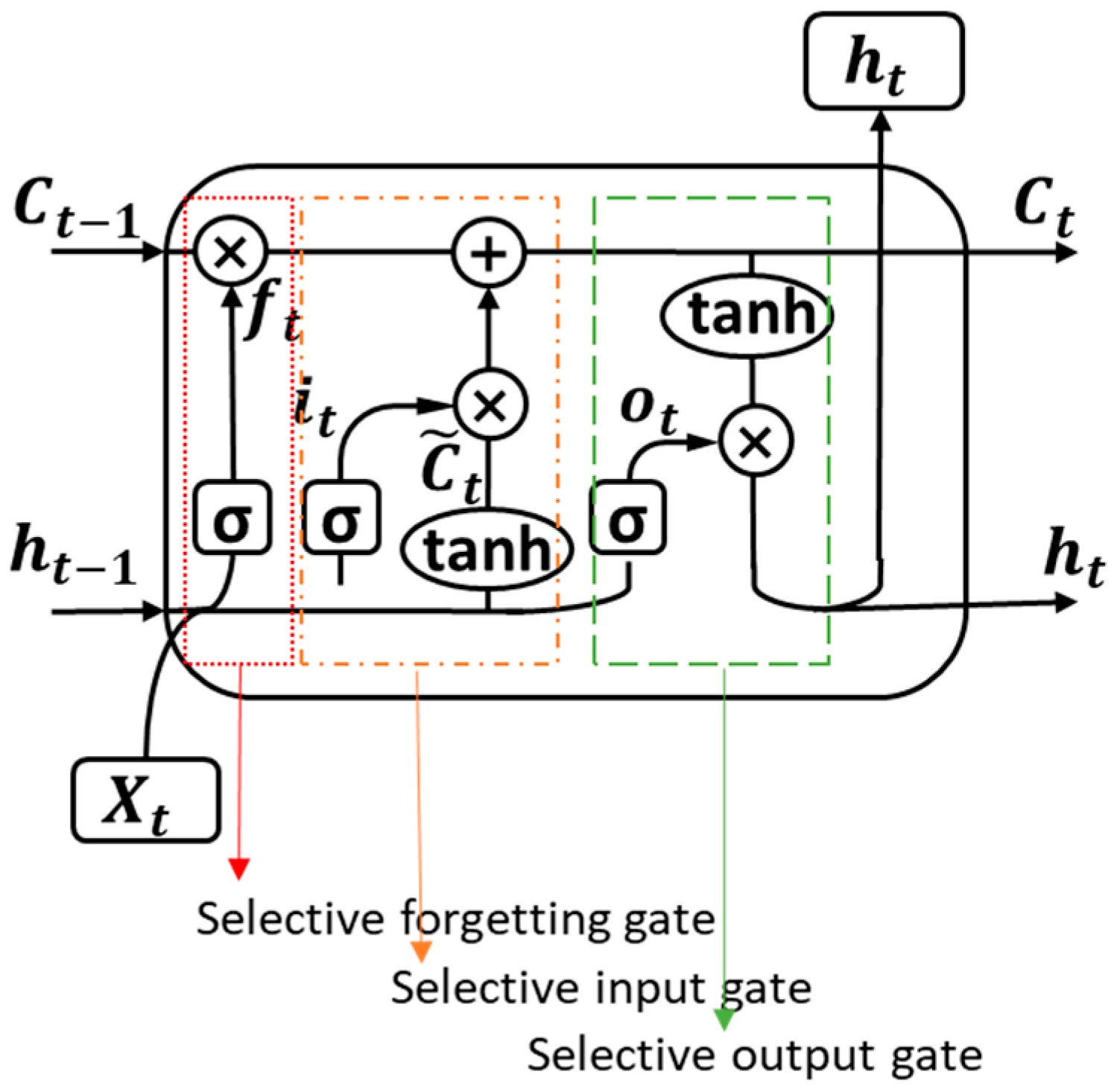
For the traditional EV energy consumption prediction, they usually simulate the EV with the driving condition of the NEDC cycle or the constant speed of 60 km/h based on the remaining energy and estimate the remaining driving range. However, this method would result in an inaccurate estimation due to the difference in actual driving. Therefore, an EV energy consumption prediction method that considers traffic information is put forward. This method replaces the NEDC driving cycle or the constant speed 60 km/h driving condition with the actual traffic environment and integrates traffic information and vehicle driving condition information, which makes the prediction of the driving energy consumption of EV more accurate. Because LSTM [29] has a special gating structure, it largely overcomes the shortcomings of the traditional recurrent neural network (RNN) [30] that the data memory of long-term sequences is not strong enough. While EV driving condition data and traffic information data are just typical domain data, here, we use the LSTM, as shown in Figure 4 to establish a deep learning-based EV energy consumption prediction model.

Where in Figure 4, $X_{\mathrm{t}}$ is the input of the current time, $h_{\mathrm{t}-1}$ is the output of the previous LSTM unit, $C_{\mathrm{t}-1}$ is the memory of the previous unit, the output of the current network is $h_{\mathrm{t}}$, and $C_{\mathrm{t}}$ is the memory of the current unit. LSTM’s forgotten gate is responsible for forgetting part of the content and the selective input gate selects part of $h_{\mathrm{t}-1}$ and $X_{\mathrm{t}}$ in order to avoid over-fitting of the model. The selective output gate implements the selective output of the internal data of the LSTM model.

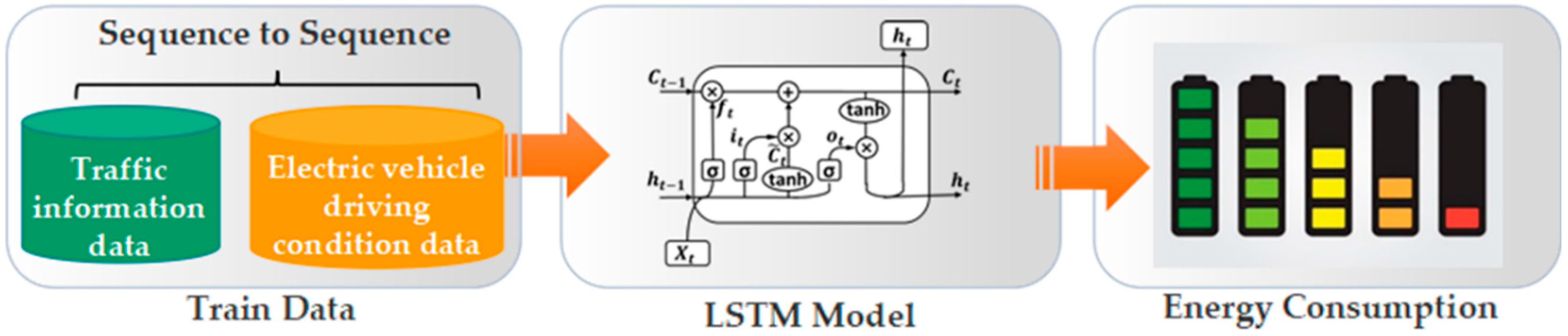
Based on LSTM, an EV energy consumption prediction model based on traffic information and vehicle driving condition information as listed in

Table 5. Training data for the LSTM model.

Traffic Information Data	Electric Vehicle Driving Condition Data
Link length	SOC0
Average speed	Road energy consumption
Average traffic flow	Battery voltage
Average traffic density	Battery current

is established, as shown in Figure 5. The sequence to sequence technology is used to realize the fusion of multi-dimensional data from transportation and electric vehicles and the result of data fusion serves as an input to LSTM. Sequence to sequence is a technique for implementing data mapping from one-dimensional sequence to another that is not the same as the original data dimension. The model takes the data as a sequence node every five minutes, takes the historical data of the first fifty-five minutes as input, and outputs the driving energy consumption of each electric vehicle in the traffic network in the next five minutes.

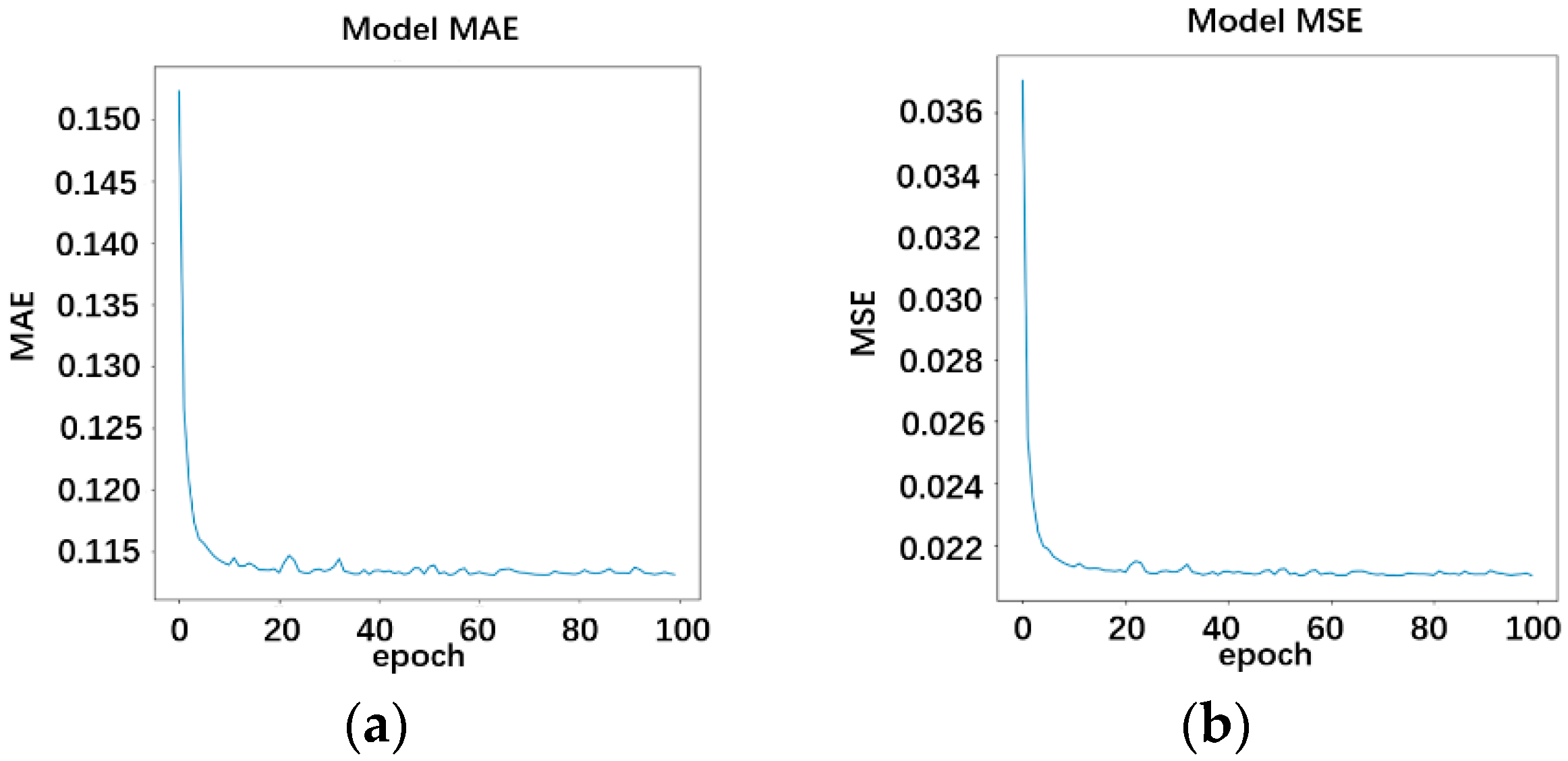
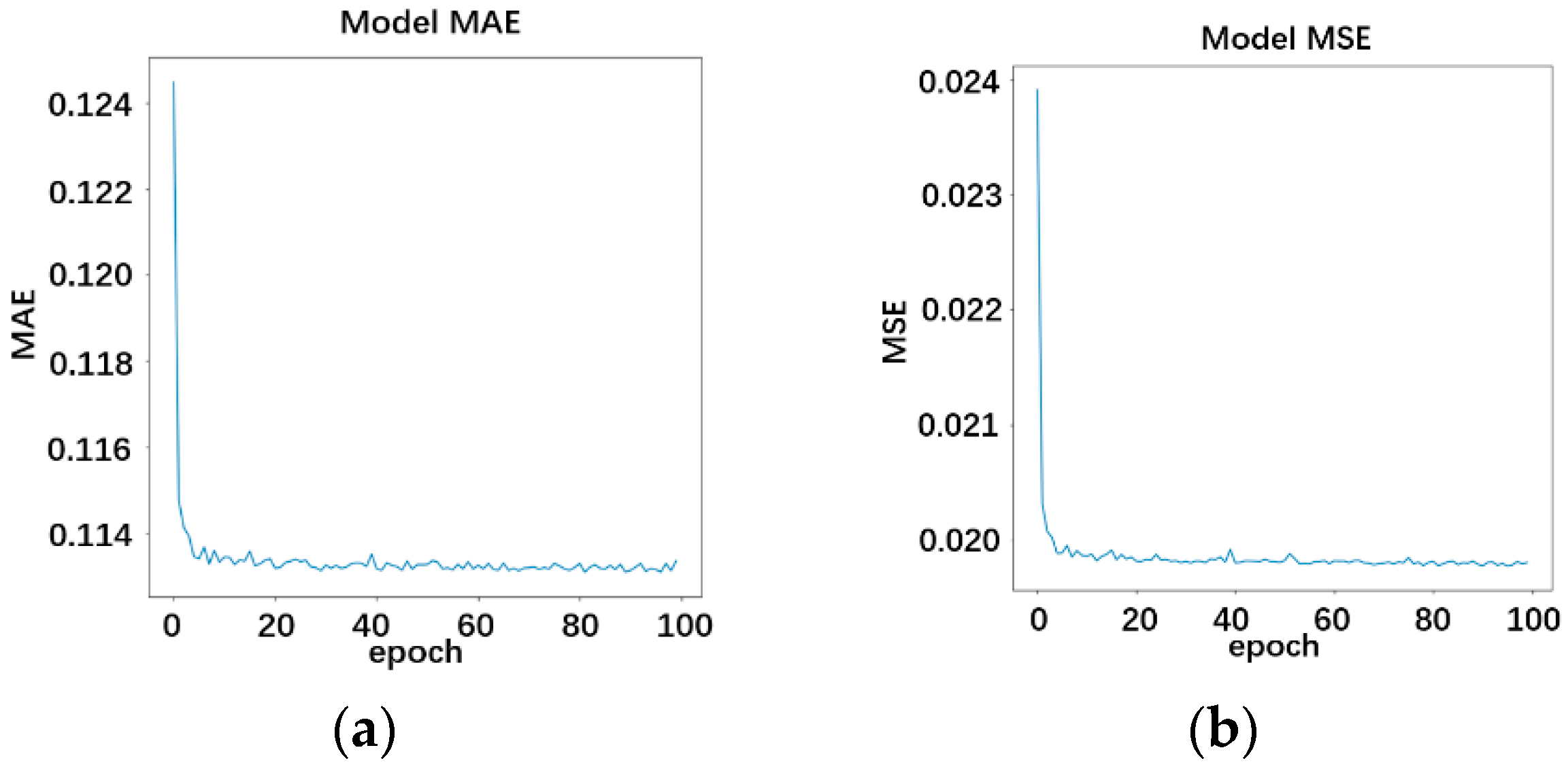
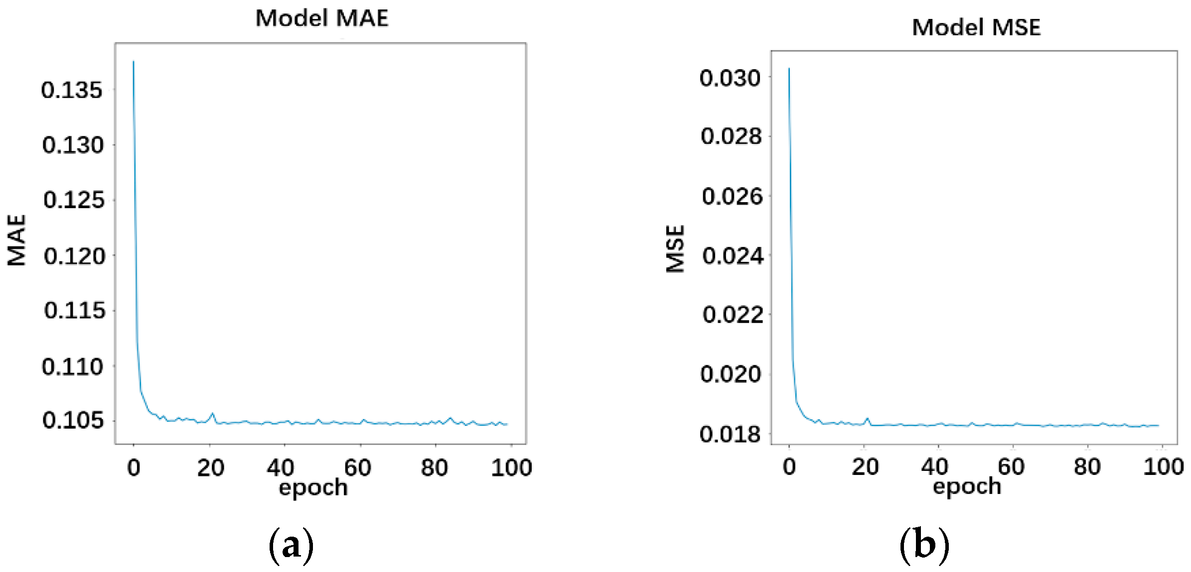
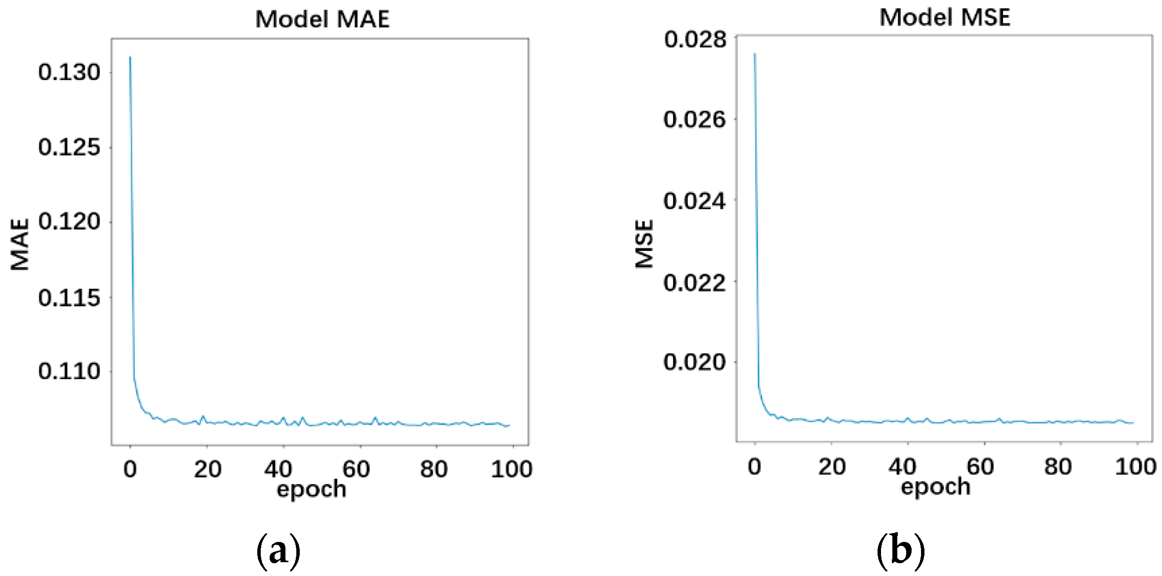
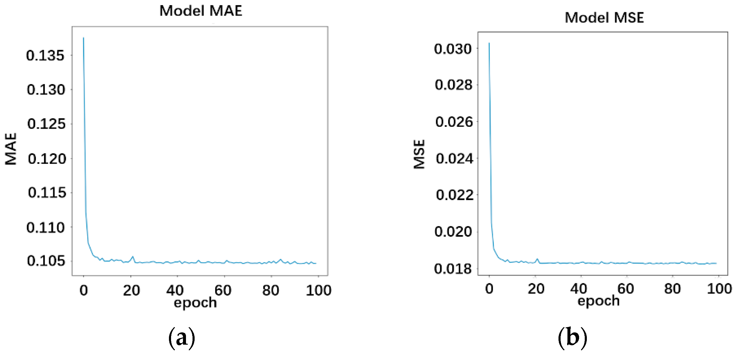
After finishing the LSTM model training, the model error is verified using the mean absolute error (MAE) and mean square error (MSE), respectively. Using experiments, the comparison variable is the number of roads in the training data, the simulation duration, and the results are listed in

Table 6. The influence of the number of roads in the model input data on the prediction results.

Road Number	Road Share	Simulation Time	MAE	MSE
33	25%	6 h	0.1159	0.0217
65	50%	6 h	0.1133	0.0196
130	100%	6 h	0.1042	0.0177

and

Table 7. The influence of different simulation durations in the model input data on the prediction results.

Road Number	Simulation Time	Simulation Time Ratio	MAE	MSE
130	2 h	33.3%	0.1091	0.0208
130	4 h	66.7%	0.1048	0.0184
130	6 h	100%	0.1042	0.0177

and shown in Figure 6, Figure 7, Figure 8, Figure 9, Figure 10 and Figure 11.

From the experimental results, the error of the LSTM model decreases with the increase of the data duration or the number of roads. When the model input is 6 h and the number of roads is 130, the error is the smallest. In the actual situation, if the training data contains more roads and longer data lengths, the model error will be much smaller. The energy consumption of the electric vehicle on each road can be updated every five minutes according to the changes of traffic conditions and the state of the electric vehicle.

5. The Planning Strategy of the Optimal Coupling Path between Energy Consumption and Distance

After finishing the energy consumption prediction of the electric vehicle, it is also necessary to construct a road resistance cost function to couple the energy consumption with the distance as shown in Equations (18)–(20). In the road resistance function, the weight of the energy consumption and the distance are both set to 50%.

$$f\left(x_1,x_2,t\right)=a\times m_{x_1,x_2,t}+b\times n_{x_1,x_2}$$

(18)

$$m_{x_1,x_2,t}=g\left(x_1,x_2,t\right)$$

(19)

$$t=5\times q\left(\min \right),q=1,2,\dots ,N$$

(20)

where $m_{x_1,x_2,t}$ is the energy consumption of road $x_1$ to road $x_2$ at time t, $n_{x_1,x_2}$ is the distance of road $x_1$ to road $x_2$, and a and b are the weighting factors, $a=b=50\%$. Since the energy consumption of road $x_1$ to road $x_2$ changes with time, and the road traffic information changes little in the 5 min time interval, this paper uses 5 min to calculate the energy consumption in one time unit, so q is the number of five minutes after departure. So the energy consumption m is a function of the starting point, the end point and the time. $f$ (x₁,x₂,t) is the road resistance cost function for energy consumption and distance.

The road resistance cost function matrix for this condition can be built as Equation (21)

$$\left[\begin{array}{ccccc}\infty & f(x_1,x_2,t)& \dots & f(x_1,x_{129},t)& f(x_1,x_{130},t)\\ f(x_2,x_1,t)& \infty & \dots & f(x_2,x_{129},t)& f(x_2,x_{130},t)\\ \dots & \dots & \infty & \dots & \dots \\ f(x_{129},x_1,t)& f(x_{129},x_2,t)& \dots & \infty & f(x_{129},x_{130},t)\\ f(x_{130},x_1,t)& f(x_{130},x_2,t)& \dots & f(x_{130},x_{129},t)& \infty \end{array}\right]$$

(21)

We also set the path of optimal energy consumption and time relative to the path with the shortest energy consumption and distance. The road resistance cost function is shown in Equations (22)–(25).

$$z\left(x_1,x_2,t\right)=c\times m_{x_1,x_2,t}+d\times T_{x_1,x_2,\mathrm{t}}$$

(22)

$$T_{x_1,x_2,\mathrm{t}}=n_{x_1,x_2}/v\_av{g}_{x_1,x_2,\mathrm{t}}$$

(23)

where $T_{x_1,x_2,t}$ is the traveling time needed from $x_1$ to $x_2$ at time t. The weighting factors c, d here we set $c=20\%,d=80\%$, because usually, people need less travel time than energy consumption. The time t and energy consumption $m_{x_1,x_2,t}$ are defined in Equations (19) and (20). $z\left(x_1,x_2,t\right)$ is the road resistance cost function for energy consumption and travel time.

The road resistance cost function matrix for this condition can be built as Equation (24).

$$\left[\begin{array}{ccccc}\infty & \mathrm{z}(x_1,x_2,t)& \dots & z(x_1,x_{129},t)& z(x_1,x_{130},t)\\ z(x_2,x_1,t)& \infty & \dots & z(x_2,x_{129},t)& z(x_2,x_{130},t)\\ \dots & \dots & \infty & \dots & \dots \\ z(x_{129},x_1,t)& z(x_{129},x_2,t)& \dots & \infty & z(x_{129},x_{130},t)\\ z(x_{130},x_1,t)& z(x_{130},x_2,t)& \dots & z(x_{130},x_{129},t)& \infty \end{array}\right]$$

(24)

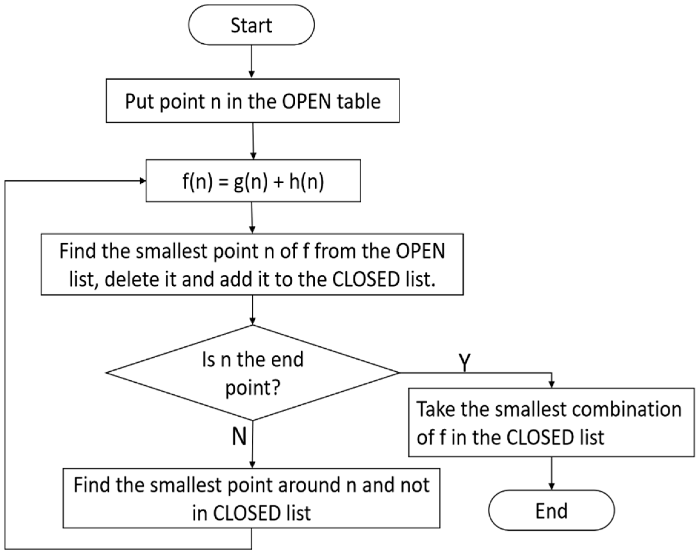
A-Star algorithm is a heuristic algorithm, as shown in Figure 12, which can determine the search scope based on the estimated value of the current point-to-end road resistance, making the search point closer and closer to the optimal point. A-Star algorithm is widely used in the scenarios of autonomous driving path planning and vehicle navigation [31]. Here we select the A-Star algorithm as the main solver, the road resistance and the traffic network obtained by the above equations are taken as inputs like matrix (21) and matrix (24), and the A-Star algorithm can output the best driving path. Take the energy consumption and driving distance as optimization goals, or take energy consumption and driving time as optimization goals to plan the economic driving path.

6. Results and Discussion

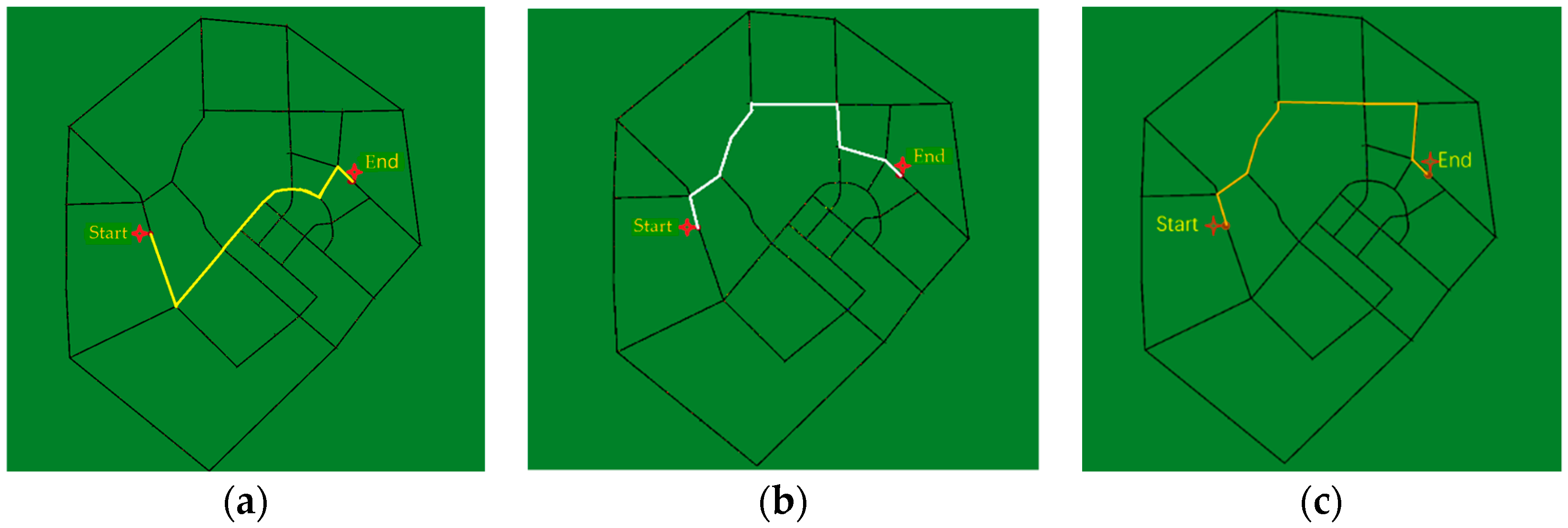
In this paper, three groups of experiments are set up, that is, distance-based, energy-based, and time-based optimal simulation experiments. The optimal distance path is used as the comparison base. The experiment of coupling the optimization of energy consumption and distance and the experiment of time optimization and energy consumption optimization are used to prove the application value of energy consumption prediction considering the traffic information in path planning.

According to the experiment results as shown in Figure 13 and

Table 8. The optimal results for different optimization conditions.

Path Type	Drive Distance	Energy Consumption	Equivalent Energy Consumption Rate	Traveling Time	Average Speed
Shortest Distance-based	3515.3 m	0.731 kWh	20.79 kWh/100 km	11.7 min	16.17 km/h
Energy saving-based	3661.8 m	0.686 kWh	18.73 kWh/100 km	7.0 min	31.39 km/h
Time saving-based	3705.6 m	0.705 kWh	19.03 kWh/100 km	5.9 min	37.68 km/h

, the shortest distance-based optimization path from the starting point to the end point is 3515.3 m, the EV consumes 0.731 kWh electricity with the equivalent energy consumption rate of 20.79 kWh/100 km and the average speed is 16.17 km/h, indicating that the road is relatively congested and the energy consumption is relatively high. For the coupling optimal energy consumption and distance path, here named as the energy saving-based optimization path, the total electricity consumption is 0.686 kWh with an equivalent energy consumption rate of 18.73 kWh/100 km, 9.9% less than the shortest distance-based optimization path and is the lowest energy consumption among the three paths. For the coupling optimal energy consumption and time path, here named as the time saving-based optimization path, its driving time is 5.9 min and is the shortest time consumption path, while its total electricity consumption is 0.705 kWh with the equivalent energy consumption rate of 19.03 kWh/100 km, 8.4% less than the shortest distance-based optimization path and 1.6% more than the energy saving-based optimization path.

7. Conclusions

(1)

The EV energy consumption model is built and verified through a test bench experiment of 3 NEDC driving cycles and actual road driving cycles. The actual traffic network is modeled with the software SUMO updated with actual traffic data. In order to predict the energy consumption accurately, a deep learning-based energy consumption prediction model with LSTM is proposed, which can fuse multi-dimensional data from different sources including traffic information. The sequence to sequence technology is used to realize the fusion of multi-dimensional data from transportation and electric vehicles. The dimensions and influence of the model training input data are also discussed with the result of 6 h long and 130 roads minimum.

(2)

A path planning map and the road resistance function are established, and the energy-saving path planning strategy with the optimal coupling of energy consumption and distance or energy consumption and driving time is proposed by the usage of the A-star algorithm. As a comparison, the shortest distance-based optimal path is also performed. The comparison results show that for the coupling optimal energy consumption and distance path, its equivalent energy consumption rate is 9.9% less than the shortest distance-based optimization path, while for the coupling optimal energy consumption and time path, it is 8.4% less than the shortest distance-based optimization path.