Research and Application of a Novel Hybrid Model Based on a Deep Neural Network Combined with Fuzzy Time Series for Energy Forecasting


Abstract
1. Introduction
- (1)
- Because physical algorithms are very sensitive to market information, they need a long run time and a large amount of computing resources. In addition, these models have shortcomings in dealing with short-term forecasting problems and they do not have high accuracy and validity in short-term forecasting.
- (2)
- Traditional statistical arithmetic methods fail to manage forecasting with fluctuations and high levels of noise, nonlinear and irregular trends, or other inherent characteristics of wind speed data that are primarily confined by the premise of a linear pattern along a time series. Moreover, oftentimes, these methods require a large amount of historical data on which they deeply depend in realistic cases. This means that once there is an abrupt and unexpected change in the original data as a result of social or environmental factors, prediction errors will proliferate all at once [38].
- (3)
- Spatial correlation arithmetic methods based on vast quantities of information, for example, the wind speed information of many spatially correlated sites which is difficult to collect and analyze, makes it hard to perform perfect wind speed forecasting [39].
- (4)
- Artificial intelligence arithmetic methods, different from other approaches, are able to deal with nonlinear features which are hidden among historical wind speed data. Although many studies have been carried out and the methods have been successfully applied to address complex data patterns, there are also some defects and drawbacks within artificial intelligence methods, such as showing a relatively low convergence rate and over-fitting, easily getting into a local optimum, etc.
- (5)
- Individual forecasting models are good at forecasting to some extent, but they rarely focus on the importance and necessity of data preprocessing; therefore, these approaches cannot always get a good forecasting outcome.
- (1).
- This study proposes a hybrid forecasting model which can take advantage of deep learning networks as well as the fuzzy time analysis technique based on the LEM2 rule-generating algorithm, which increases the forecasting accuracy obviously. To our knowledge, it has not been found that deep leaning neural networks are combined with the rough set induction theory. Hence, our study develops a hybrid model combining LSTM with the fuzzy time series analysis technique that uses rough sets to generate rules as a replacement for traditional rule-generating methods.
- (2).
- This study improves the forecasting stability and accuracy simultaneously with the deep learning neural network through the weight-determining method called MOGWO based on the leave-one-out strategy and swarm intelligence, which helps to find best weighting parameters for the LSTM neural network. Most previous studies just paid attention to one aim (stability or accuracy). Therefore, to achieve high accuracy and stability, a multi-objective optimization algorithm, MOGWO, is successfully applied in this study.
- (3).
- This study provides a scientific and reasonable evaluation of the new hybrid forecasting model made to verify the forecasting performance of the combined forecasting model proposed in this paper. Three experiments are carried out in this paper, including comparisons between different deep learning neutral networks, efficiency and effectiveness tests among various models in four different wind sites, and a contrast experiment in which the proposed hybrid forecasting system is applied to electrical load forecasting with two different electrical power load data series on Wednesday and Sunday. The outcome illustrates that this proposed system performs well.
- (4).
- This study delivers an insightful discussion about the developed forecasting system, illustrating the improvements brought about by different parts of the proposed forecasting model as well as the multistep forecasting ability. Five discussion topics are presented in this paper, namely statistical significance, association strength, improvement percentage, multistep ahead forecasting, and sensitivity analysis. Through these discussions, the effectiveness of the hybrid forecasting framework is verified.
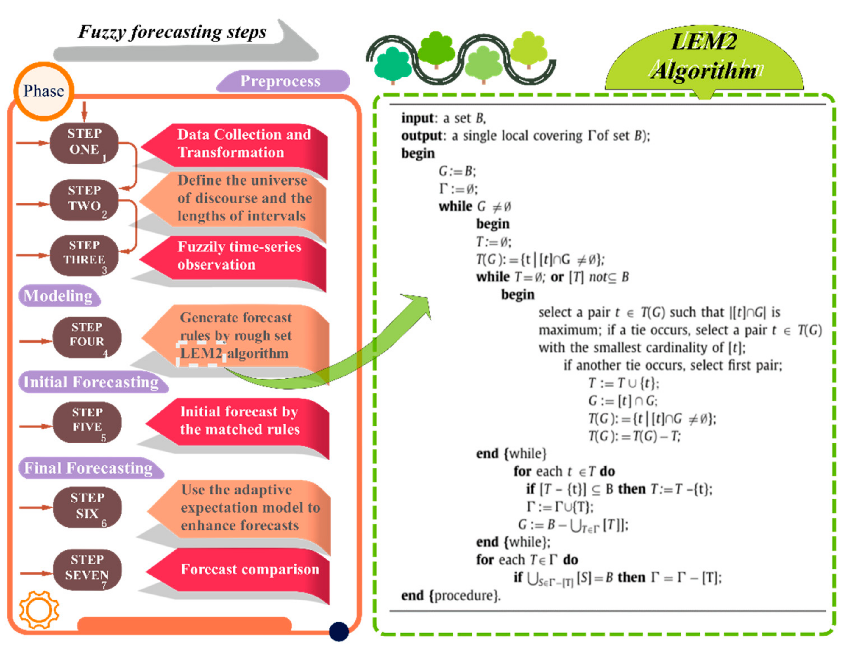
2. Methodology
2.1. Hybrid Forecasting Framework
- The original wind speed data is decomposed by applying the CEEMD method into several subseries named Intrinsic Mode Functions (IMFs).
- The fuzzy analysis method is applied using the rough set induction LEM2 algorithm to generate the forecasting rules, and raw data are applied to these rules to generate preliminary forecasts. These forecasts obtained by fuzzy time series forecasting are not precise enough, but the difference between these forecasts and the actual values can demonstrate potential forecasting biases that are useful for modifying the learning process of the following neural network, namely the LSTM model optimized with MOGWO. As for the raw input data, we accept five dimensions for each forecast, including lag1, lag2, lag3, slope, and the present data, in order to forecast the following one for each subseries (Figure 2).
- The output data generated from the previous steps is used as the input data for the LSTM forecasting module, which is optimized by the multi-objective optimization algorithm called MOGWO for each subseries. Specifically, real values of lag1, and lag2 and their differences, including D1, D2, and D3, are adopted as input data of the LSTM model modified by MOGWO (Table 1).
- The forecasting outcomes of each subseries generated from the preprocessing part named CEEMD are aggregated to obtain the eventual forecasting results of CFML.
2.2. Data Preprocessing Module
- Step 1:
- Add white noise pairwise with the identical amplitude and the opposite phase to the raw data sequence , after which we can obtain a pair of polluted signals:
- Step 2:
- Decompose the polluted signal pairs () into a finite set including IMF components:
- Step 3:
- Two sets of IMF components, i.e., the negative noise set of the first IMF component and positive noises , are obtained by performing the above two steps T times with different amounts of white noise.
- Step 4:
- The component of the j-th IMF can be calculated as follows in order to get the ensemble means of whole IMFs:
2.3. Rough Set Theory (RST) and LEM2
- 1.
- Rough sets can discern hidden facts and make it possible for us to understand these facts in natural language, which contributes a great deal to decision making;
- 2.
- Rough sets take the background information of decision makers into account;
- 3.
- Rough sets can deal with both qualitative and quantitative attributes;
- 4.
- Rough sets enable machines to extract certain rules in a relatively short time, which means it reduces the time cost of discovering hidden rules.
- Step 1.
- Compute all attribute–value pair blocks.
- Step 2.
- Identify attribute–value pairs with the largest .
- Step 3.
- If the cardinality of the set is equal to another one, then select the attribute pair with the smallest block size.
- Step 4.
- If necessary, we have to go through an additional internal loop in order to find the candidates for the minimal complex.
- Step 5.
- Then, the following steps are used to find the second minimal complex and so on.
- Step 6.
- Finally, we can get the local covering of a hidden fact, which may reveal the decision-making process.
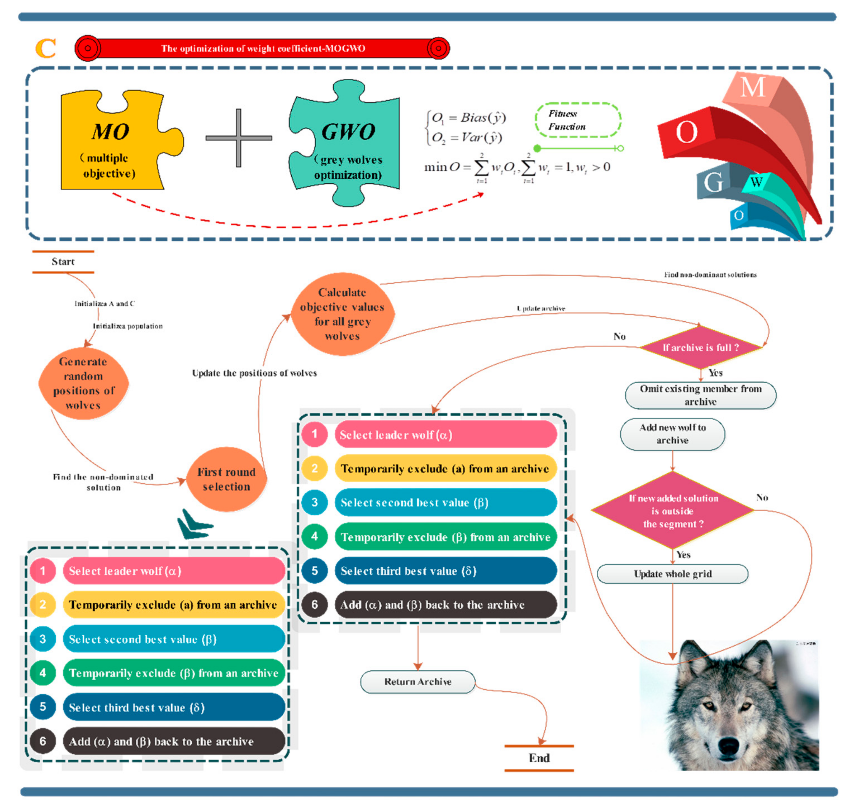
2.4. Multi-Objective Grey Wolf Optimizer (MOGWO)
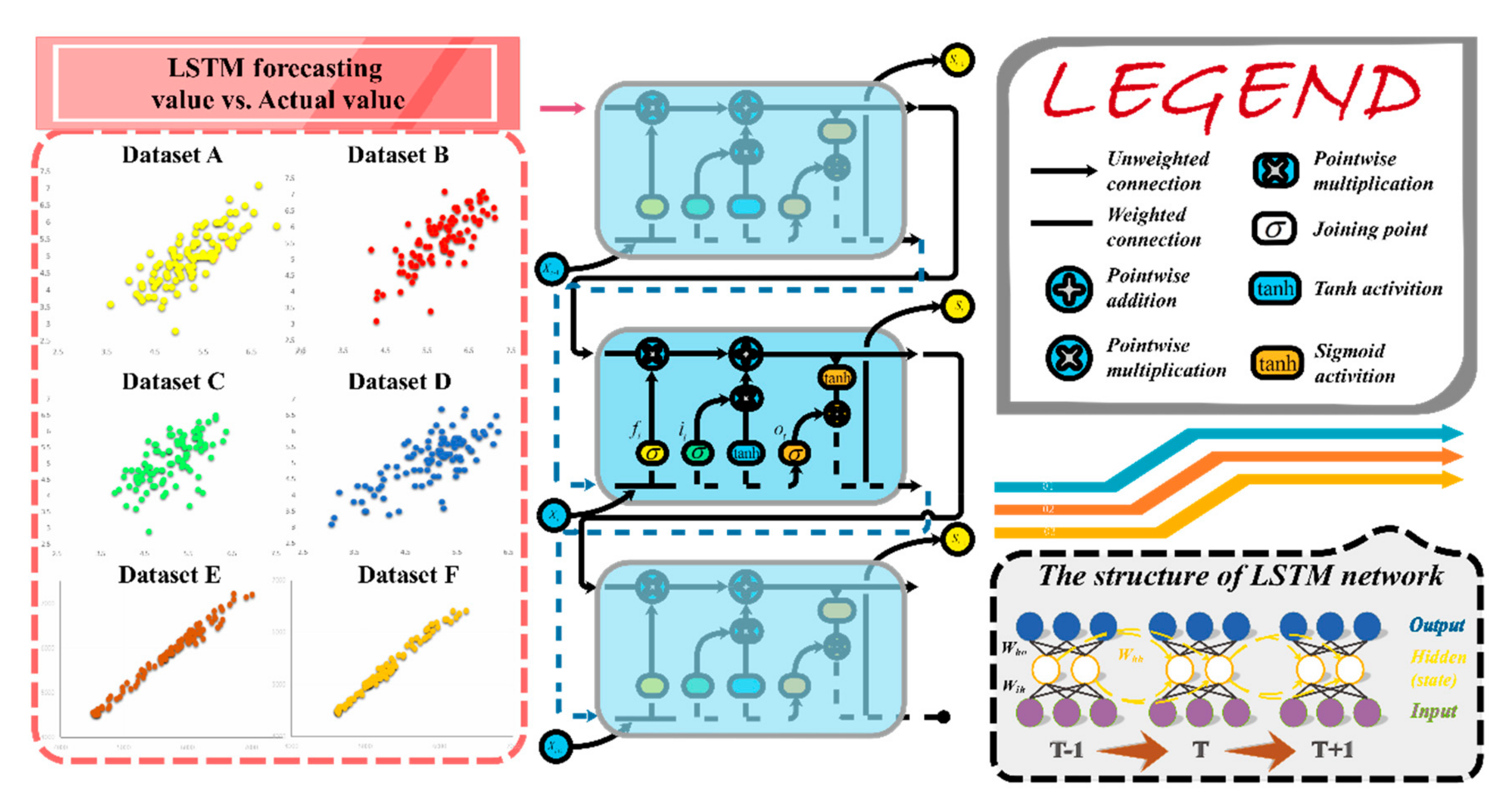
2.5. Long Short-Term Memory (LSTM)
- In the LSTM module, the first step is to determine which information will be discarded from the cell state. The forget gate () is in charge of making decisions, as follows:where σ is the sigmoid function which turns the input value into an outcome between 0 and 1. T signifies weight parameters, and b denotes bias parameters (i.e., , , , and and ,, , and ). In this part, the exponents of T and V are not power values; they are just notations used to illustrate which gate the parameters belong to. For instance, represents the weight parameters belonging to the forget gate, namely gate f.
- The next step is to determine which new information will be selected and stored in the cell state. This step has two sub-steps: The first one is the input gate () layer that helps to determine which value is going to be updated. A tanh layer is the second one, which produces a vector composed of new candidate values . Calculations are demonstrated as follows:where is a candidate memory cell, which is similar to a memory cell, but uses a tanh function.
- The next step is to update the old cell state into the new cell state , which can be described as follows:In Equation (26), the symbol represents pointwise multiplication.
- The final step is to determine what is about to be generated and selected as the output. This output is a filtered version which is predicated on the cell state, during which the output gate () determines which final output will consist of a specific part of the cell state. After, the cell state runs through the tanh layer, which is multiplied by the output gate as follows:
| Algorithm: MOGWO-LSTM | |
| Objective function Input: | |
| Training data: | |
| Testing data: | |
| Output: | |
| —a series of forecasting data | |
| Parameters of MOGWO: | |
| Iter—the maximum number of iterations | n—the number of grey wolves |
| t—the current iteration number | Ri—the position of wolf i |
| e1—the random vector in [0, 1] | c—the constant vector in [0, 2] |
| Parameters of LSTM: | |
| Iteration—the maximum number of iterations | Bias_input—the bias vector of the input gate in [0, 1] |
| Input_num—the knots of the input | Bias_forget—the bias vector of the forget gate in [0, 1] |
| Cell_num—the knots of the cell | Bias_output—the bias vector of the output gate in [0, 1] |
| Output_num—the knots of the output Cost_gate—the termination error cost | yita—the rate of adjustment for the weight at each time data_num-the number of columns of training data. |
| 1:/*Set the parameters of MOGWO and LSTM*/ | |
| 2:/*Initialize the grey wolf population Ri (i = 1, 2, ..., n) randomly*/ | |
| 3:/*Initialize c, M, and B*/ | |
| 4:/*Define the archive size*/ | |
| 5: FOR EACH i: 1 ≤ i ≤ n DO | |
| 6: Evaluate the corresponding fitness function Fi for each search agent | |
| 7: END FOR | |
| 8: /*Find the non-dominated solutions and initialize the archive with them*/ | |
| 9: Rα, Rβ, Rδ= SelectLeader(archive) | |
| 10: WHILE (t < Iter) DO | |
| 11: FOR EACH i: 1 ≤ i ≤ n DO | |
| 12: /*Update the position of the current search agent*/ | |
| 13: Kj = |Bi Rj−R|, i = 1, 2, 3; j = α, β, δ | |
| 14: Ri = Rj−Mi Kj, i = 1, 2, 3; j = α, β, δ | |
| 15: R(t + 1) = (R1 + R2 + R3)/3 | |
| 16: END FOR | |
| 17: /*Update c, M, and B*/ | |
| 18: M = 2 c e1−c; B = 2 c e2−c | |
| 19: /*Evaluate the corresponding fitness function Fi for each search agent*/ | |
| 20: /*Find the non-dominated solutions*/ | |
| 21: /*Update the archive with regard to the obtained non-dominated solutions*/ | |
| 22: IF the archive is full DO | |
| 23: /*Delete one solution from the current archive members*/ | |
| 24: /*Add the new solution to the archive*/ | |
| 25: END IF | |
| 26: IF any newly added solutions to the archive are outside the hypercubes DO | |
| 27: /*Update the grids to cover the new solution(s)*/ | |
| 28: END IF | |
| 29: Rα, Rβ, Rδ = SelectLeader(archive) | |
| 30: t = t + 1 | |
| 31: END WHILE | |
| 32: RETURN archive | |
| 33: OBTAIN R* = SelectLeader(archive) | |
| 34: Set R* as the initial weight and threshold of LSTM | |
| 35: /*Standardize the training data and testing data*/ | |
| 36: /*Initialize the structure of the LSTM network*/ 37:/*Initialize cost_gate, bias_input, bias_forget, bias_output and the weight of the LSTM network*/ 38: FOR EACH i: 1 ≤ i ≤ Iteration DO 39: yita=0.01 40: FOR EACH m: 1 ≤ m ≤ data_num DO 41: Equation (15) to Equation (20) 42: /*Calculate the error cost of this round*/ 43: error cost = l is the dimension of testing data 44: IF error cost < cost_gate DO 45: Break 46: END IF 47: /*Update the weight of all gates*/ 48: END FOR 49: IF error cost < cost_gate DO 50: Break 51: END IF 52: END FOR 53: /* Learning process has been done/ 54: Input the standardized historical data into LSTM to forecast the future changes 55: De-normalize the obtained forecasting outcomes and generate the final forecasting results | |
2.6. Evaluation Module
2.6.1. Typical Performance Metric
2.6.2. Diebold–Mariano Test
3. Analysis and Experiments
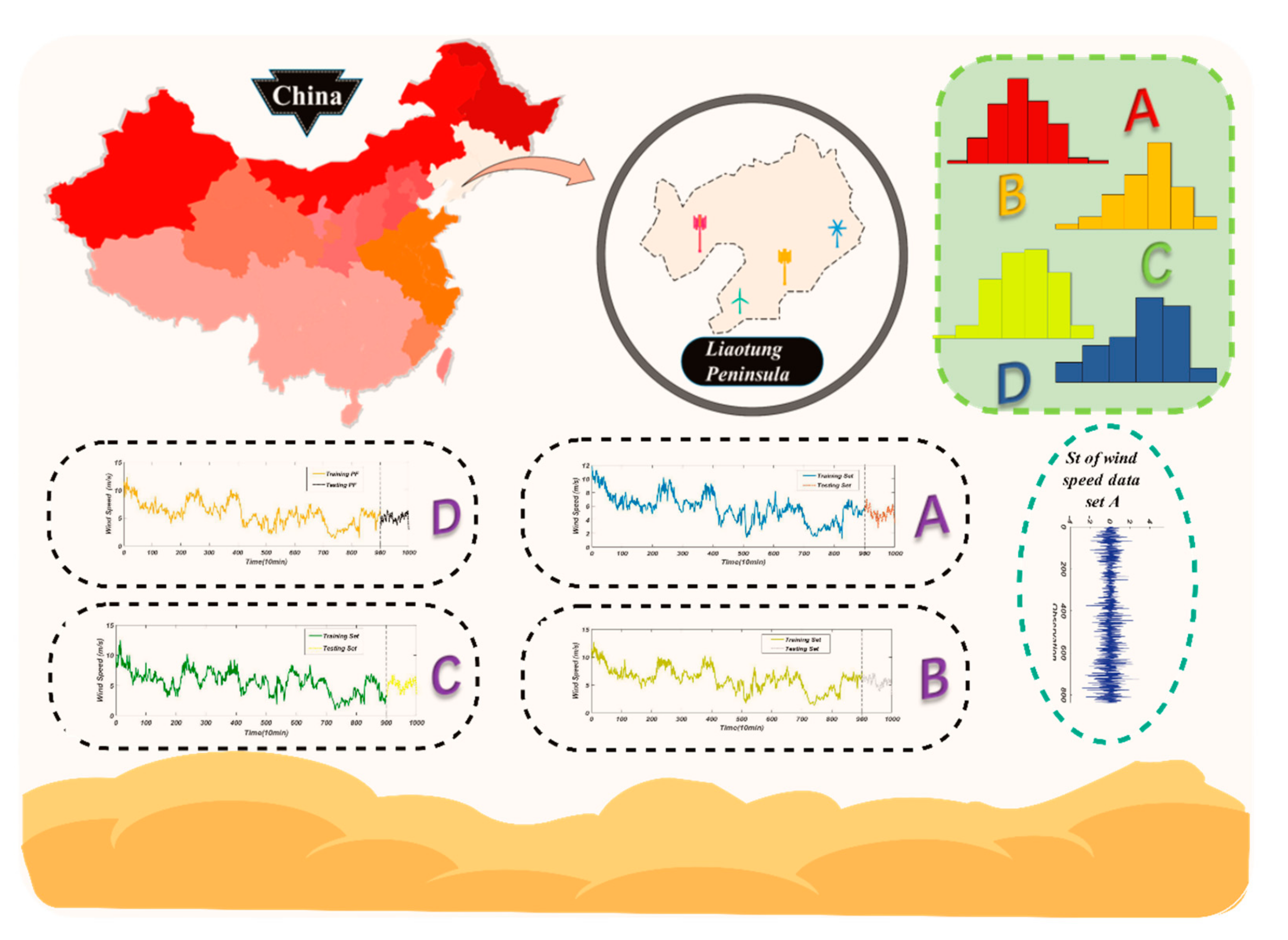
3.1. Raw Data Description
3.2. Experiment I: Tests of MOGWO and LSTM
3.2.1. Test of MOGWO
- The MOGWO algorithm obtained the best IGD outcomes among almost all optimizers for four test functions (Kursawe, ZDT1, ZDT2, and ZDT3) while performing worse than the Kursawe as well as ZDT1 algorithms in terms of the minimum value and worse than MODA regarding the standard deviation. From a whole perspective, these outcomes are strong enough to demonstrate the superior optimization ability of MOGWO algorithms compared with the others.
- Figure 7 shows that the MOGWO algorithm was able to obtain more Pareto optimal solutions. In addition, the solutions found by the MOGWO algorithm were more evenly distributed on the true PF (pareto front) curve and were closer to the real Pareto optimal solutions.
3.2.2. Test of LSTM in CEEMD-FTS-MOGWO-LSTM
- The LSTM model achieved almost the best results and the most accurate predictions of all four wind speed datasets with roughly the same run time and identical training and testing datasets. Namely, the adopted LSTM model outperformed the CNN, DBN, and SAE from a whole perspective and provided fairly competitive results.
- For the data collected from the four different wind farms, the LSTM model worked better than the other three deep learning models, which means that the superiority of the LSTM forecasting algorithm remained, regardless of the different geographical distribution, to some extent.
- The forecasting performance of different models was adequately reflected by the error metrics adopted by us in this part. That is to say, error measurement is effective and can be used to accurately evaluate the ability of the prediction models.
3.3. Experiment II
- (1)
- For the first comparison, WNN, GRNN, ARIMA, and the LSTM models were built and compared with each other in order to determine the best one for performing wind speed forecasting, which was found to be the ARIMA. However, of all the neural network algorithms, LSTM was shown to be the best one, and Experiment I proved that LSTM is better than the other three deep learning models as well. Hence, the following steps and comparisons are all based on the basic and regular forecasting model—LSTM.
- (2)
- In terms of R (Pearson’s correlation coefficient), ARIMA failed to outdo LSTM in datasets A and B. In addition, we tried AR, MA, ARMA, and ARIMA with different parameters each, and we found that of all these settings, ARMA(2,1), ARIMA(3,1,2), and ARIMA(3,2,2), achieved almost the same forecasting accuracy at about 8% MAPE, which is apparently better than that of the other neural networks. The reason for this phenomenon is that the moving-average model that includes AR requires clear rhythm patterns and fairly linear data series trends, whereas wind speed datasets are neither seasonal nor regular, so all of these irregular features were almost removed by the moving-average method as a result of the differencing operation.
- (3)
- From Table 7, for example, the MOGWO-LSTM achieved a MAPE value of 8.64%, while the basic LSTM model only achieved a MAPE value of 9.48% in the case of site A. Moreover, we tested the effectiveness of the fuzzy time series forecasting part. For example, in the case of site B, the MAPE value of FTS-LSTM was 7.91%, 8.34% lower than that of the LSTM model.
- (4)
- According to Figure 8, the FTS-MOGWO-LSTM model achieved 8.02% in MAPE and 75.34% in r2 from a mean perspective, although it failed to reach the highest r2 value in datasets A and B. Next, the separate improvement on the forecasting ability brought by FTS or MOGWO varied in different datasets. For example, in the case of dataset A, FTS-LSTM was higher than MOGWO-LSTM, which means that MOGWO contributes more to forecasting.
- (5)
- Apart from these comparisons, the decomposition algorithm was also tested in this part. In this paper, we tested several parameter configurations regarding the Nstd (signal noise ratio), NR (noise addition number), Maxiter (maximum number of iterations), and modes (number of IMFs) in the CEEMD algorithm. We tested the Nstd (0.05–0.4), NR (10–500), Maxiter (100–1000), and modes (9–13) to find the best configuration. Detailed parameter settings vary from dataset to dataset, so settings should be changed at any time when the dataset is changed. In this part, for instance, the best settings for dataset A were as follows: an Nstd of 0.2, an NR of 50, and a Maxiter of 500. The total IMF number was 12, and the best accuracy is acquired by 11 IMFs. Also, Table 8 shows that the CFML model achieved the highest r2 value and the lowest MAPE in all four data sites, which demonstrates the improvements brought by CEEMD.
3.4. Experiment III: Tested with Electrical Load Data
- (1)
- Regarding the electrical power load data from Wednesday and all forecasting steps, the proposed hybrid forecasting system performed the best among all the other models. Moreover, among all the single models involved in this experiment, the single model that performed best was the WNN algorithm, while the worst was the CNN model. However, this may be a result of the data features, which does not mean that the CNN constantly performs more poorly than the WNN model. Since the regular form of the CNN model is designed to deal with figure data, to perform unidimensional time series forecasting, it should be first transformed into a matrix in which each row contains many observations, such as 128 or 256, just like the grey scale image data to some extent. Otherwise, it is also reasonable and practical to let each row represent the number you would like to use as input data, but a compromise in the accuracy may arise on some occasions.
- (2)
- For the test of the optimization part and the verification of the fuzzy forecasting part, comparisons between MOGWO-LSTM and LSTM and comparisons between FTS-LSTM and LSTM are obviously shown in the aforementioned tables and figures, respectively. For instance, on Wednesday, the regular LSTM model achieved a MAPE of 2.81%, which is higher than the MAPE of FTS-LSTM by 39.14%. Moreover, the MOGWO-LSTM increased by 37.36% in terms of the MAPE of 1.76%. Also, the FTS-MOGWO-LSTM model possessed a MAPE of 1.46%, lower than that of the single LSTM combined with FTS or MOGWO. Noticeably, although this combined model did not have that highest r2, it was not obviously lower than that of other compared models. Moreover, it was apparently higher than that of regular networks such as GRNN, WNN, DBN, SAE, and so on.
- (3)
- All comparisons for the electrical power load data on Wednesday and Sunday demonstrate that the decomposition methods achieved the best forecasting results. In this study, we tested different parameter settings regarding the Nstd, NR, Maxiter, and modes for EMD, EEMD, and CEEMD. The following outcomes were all acquired based on the best parameter settings for each decomposition algorithm. Table 9 and Table 10 show that the CEEMD method apparently outweighs the EEMD and EMD methods, which explains why the CEEMD was selected by us and employed in this research. Also, from Figure 10, the forecasts gained by the CEEMD model corresponded most to the real data on both Wednesday and Sunday.
4. Discussion
4.1. Discussion I: Statistical Significance
4.2. Discussion II: Association Strength
4.3. Discussion III: Improvement Percentage
- (1)
- By contrasting the improvement percentage between FTS-MOGWO-LSTM with FTS-LSTM and MOGWO-LSTM, we drew the conclusion that the combination of MOGWO and FTS contributes more than either FTS-LSTM or MOGWO-LSTM to the forecasting ability of the whole presented hybrid CFML forecasting model.
- (2)
- The comparison between the CEEMD-FTS-MOGWO-LSTM and the FTS-MOGWO-LSTM models obviously revealed the improvement brought by the addition of the decomposition approach CEEMD.
- (3)
- On average, all improvement percentages were positive and significant, except for the percentages of FTS-MOGWO-LSTM, as it fluctuated according to different datasets with different features. This can be studied in the future. Regardless of the fluctuations, all values revealed that FTS-MOGWO-LSTM does perform better than the regular one.
4.4. Discussion Ⅳ: Multistep-Ahead Forecasting
4.5. Discussion V: Sensitivity Analysis
- (1)
- The value of MAPE first decreased as the number of search agents increased. Then, it declined to the minimum value with 10 search agents, after which it started increasing and fluctuated at a high level except for a decrease at 25 search agents. Overall, we can see that the proposed hybrid CFML forecasting model performed the best with 10 search agents.
- (2)
- Keeping the number of search agents at the best value of 10, we changed the number of iterations in order to check the influence caused by the iterations on the performance of the presented model. We almost drew a similar conclusion to that of the search agents to some degree. We can see that, as the number of iterations increased from 5 to 30, the accuracy measured by various metrics, especially MAPE, first fell to the minimum value with 10 iterations and then rose gradually as the number of iteration increased. According to these two conclusions, we set the number of search agents and the number of iterations to 10 in our experiment.
- (3)
- It was found through the comparisons that the number of those two parameters would worsen the performance of the CEEMD-FTS-MOGWO-LSTM system proposed in this study if either they were too small or too big. In addition, different prediction conditions were shown to depend to a large extent on the decision-making process. Therefore, it is important to figure out the optimal parameters under different application conditions.
5. Conclusions
Author Contributions
Funding
Conflicts of Interest
Abbreviations
| List of Abbreviations | FB | The fractional bias | |
| U1 | The Theil U statistic 1 | ||
| CFML | CEEMD-FTS-MOGWO-LSTM | U2 | The Theil U statistic 2 |
| WNN | Wavelet Neutral Network | DA | The direction accuracy |
| GRNN | Generalized Regression Neural Network | INDEX | The improvement ratio of the index among different models |
| SAE | Sparse Autoencoder | R2 | The Pearson’s correlation coefficient |
| LSTM | Long Short-Term Memory | DM | Diebold–Mariano test |
| DBN | Deep Belief Network | H0 | The null hypothesis |
| CNN | Convolutional Neural Network | H1 | The alternative hypothesis |
| IGD | The inverted generational distance | α | The confidence level |
| FTS | Fuzzy time series | Xt | An input at time t |
| LEM2 | Learning from examples module version two | St | The hidden state |
| AR | Autoregressive model | MA | Moving-average model |
| ARIMA | Autoregressive Integrated Moving Average | ARMA | Autoregressive moving average model |
| MODA | Multi-objective dragonfly | St−1 | The previous time step |
| MOGWO | Multi-objective grey wolf | ft | The forget gate |
| NSGA-Ⅱ | Non-dominated sorted genetic algorithm-Ⅱ | it | The input gate |
| Kα | The distance between wolf α and the prey | R1 | The position of wolf α at time ite+1 |
| Kβ | The distance between wolf β and the prey | R2 | The position of wolf β at time ite+1 |
| Kδ | The distance between wolf δ and the prey | R3 | The position of wolf δ at time ite+1 |
| QLD | Queensland | Ct−1 | The old cell state |
| Pni | Positive noise | Nni | Negative noise |
| AE | The average error | Wni | Noise with identical amplitude and phase |
| MAE | The mean absolute error | Ot | The output gate |
| RMSE | The root-mean-square error | gj | The j-th inequality constraint |
| NMSE | The normalized average of the squares of error | hj | The j-th equality constraint |
| MAPE | The mean absolute percentage error | RST | Rough set theory |
| IMF | Intrinsic mode function | IA | The index of agreement |
| ZDT2 | Zitzler–Deb–Thiele’s function N. 2 | ZDT1 | Zitzler–Deb–Thiele’s function N. 1 |
| Kursawe | Kursawe function | ZDT3 | Zitzler–Deb–Thiele’s function N. 3 |
| EMD | Empirical Mode Decomposition | ||
| EEMD | Ensemble Empirical Mode Decomposition | ||
| CEEMD | Complete Ensemble Empirical Mode Decomposition | ||
References
- Ou, T.C. A novel unsymmetrical faults analysis for microgrid distribution system. Int. J. Electr. Power Energy Syst. 2012, 43, 1017–1024. [Google Scholar] [CrossRef]
- Ou, T.C. Ground fault current analysis with a direct building algorithm for microgrid distribution. Int. J. Electr. Power Energy Syst. 2013, 53, 867–875. [Google Scholar] [CrossRef]
- Lin, W.M.; Ou, T.C. Unbalanced distribution network fault analysis with hybrid compensation. IET Gener. Transm. Distrib. 2010, 5, 92–100. [Google Scholar] [CrossRef]
- Ou, T.C.; Lu, K.H.; Huang, C.J. Improvement of transient stability in a hybrid power multi-system using a designed NIDC (novel intelligent damping controller). Energies 2017, 10, 488. [Google Scholar] [CrossRef]
- Ye, S.; Zhu, G.; Xiao, Z. Long term load forecasting and recommendations for china based on support vector regression. Energy Power Eng. 2012, 4, 380–385. [Google Scholar] [CrossRef]
- He, Q.; Wang, J.; Haiyan Lu, H. A hybrid system for short-term wind speed forecasting. Appl. Energy 2018, 226, 756–771. [Google Scholar] [CrossRef]
- Yang, W.; Wang, J.; Lu, H. Hybrid wind energy forecasting and analysis system based on divide and conquer scheme: A case study in China. J. Clean. Prod. 2019, 222, 942–959. [Google Scholar] [CrossRef]
- Abdel-Aal, R.E.; Elhadidy, M.A.; Shaahid, S.M. Modeling and forecasting the mean hourly wind speed time series using GMDH-based abductive networks. Renew. Energy 2009, 34, 1686–1699. [Google Scholar] [CrossRef]
- Wang, J.; Niu, T.; Lu, H.; Yang, W.; Du, P. A Novel Framework of Reservoir Computing for Deterministic and Probabilistic Wind Power Forecasting. IEEE Trans. Sustain. Energy 2019. [Google Scholar] [CrossRef]
- Ma, L.; Luan, S.Y.; Jiang, C.W.; Liu, H.L.; Zhang, Y. A review on the forecasting of wind speed and generated power. Renew. Sustain. Energy Rev. 2009, 13, 915–920. [Google Scholar]
- Cardenas-Barrera, J.L.; Meng, J.; Castillo-Guerra, E.; Chang, L. A neural networkapproach to multi-step-ahead, short-term wind speed forecasting. IEEE 2013, 2, 243–248. [Google Scholar]
- Torres, J.L.; García, A.; Blas, M.D.; Francisco, A.D. Forecast of hourly average wind speed with arma models in navarre (Spain). Sol. Energy 2005, 79, 65–77. [Google Scholar] [CrossRef]
- Liu, H.; Tian, H.Q.; Li, Y.F. An emd-recursive arima method to predict wind speed for railway strong wind warning system. J. Wind Eng. Ind. Aerodynam. 2015, 141, 27–38. [Google Scholar] [CrossRef]
- Kavasseri, R.G.; Seetharaman, K. Day-ahead wind speed forecasting using arima models. Renew. Energy 2009, 34, 1388–1393. [Google Scholar] [CrossRef]
- Yang, D.; Sharma, V.; Ye, Z.; Lim, L.I.; Zhao, L.; Aryaputera, A.W. Forecasting of global horizontal irradiance by exponential smoothing, using decompositions. Energy 2015, 81, 111–119. [Google Scholar] [CrossRef]
- Li, Y.; Ling, L.; Chen, J. Combined grey prediction fuzzy control law with application to road tunnel ventilation system. J. Appl. Res. Technol. 2015, 13, 313–320. [Google Scholar] [CrossRef]
- Barbounis, T.G.; Theocharis, J.B. A locally recurrent fuzzy neural network with application to the wind speed prediction using spatial correlation. Neurocomputing 2007, 70, 1525–1542. [Google Scholar] [CrossRef]
- Guo, Z.H.; Wu, J.; Lu, H.Y.; Wang, J.Z. A case study on a hybrid wind speed forecasting method using BP neural network. Knowl. Based Syst. 2011, 24, 1048–1056. [Google Scholar] [CrossRef]
- Li, G.; Shi, J. On comparing three artificial neural networks for wind speed forecasting. Appl. Energy 2010, 87, 2313–2320. [Google Scholar] [CrossRef]
- Jiang, P.; Liu, F.; Song, Y.L. A hybrid forecasting model based on date-framework strategy and improved feature selection technology for short-term load forecasting. Energy 2017, 119, 694–709. [Google Scholar] [CrossRef]
- Hao, Y.; Tian, C. The study and application of a novel hybrid system for air quality early-warning. Appl. Soft Comput. 2019, 74, 729–746. [Google Scholar] [CrossRef]
- Zhang, X.; Wang, J.; Gao, Y. A hybrid short-term electricity price forecasting framework: Cuckoo search-based feature selection with singular spectrum analysis and SVM. Energy Econ. 2019, 81, 899–913. [Google Scholar] [CrossRef]
- Lago, J.; Ridder, F.D.; Schutter, B.D. Forecasting spot electricity prices: Deep learning approaches and empirical comparison of traditional algorithms. Appl. Energy 2018, 221, 386–405. [Google Scholar] [CrossRef]
- Hinton, G.E.; Osindero, S.; Teh, Y.W. A fast learning algorithm for deep belief nets. Neural Comput. 2006, 18, 1527–1554. [Google Scholar] [CrossRef] [PubMed]
- Ni, K.L.; Wang, J.; Tang, G.J.; Wei, D.X. Research and Application of a Novel Hybrid Model Based on a Deep Neural Network for Electricity Load Forecasting: A Case Study in Australia. Energies 2019, 12, 2467. [Google Scholar] [CrossRef]
- Fischer, T.; Krauss, C. Deep learning with long short-term memory networks for financial market predictions. Eur. J. Oper. Res. 2018, 270, 654–669. [Google Scholar] [CrossRef]
- Khatami, A.; Khosravi, A.; Nguyen, T.; Lim, C.P.; Nahavandi, S. Medical image analysis using wavelet transform and deep belief networks. Expert Syst. Appl. 2017, 86, 190–198. [Google Scholar] [CrossRef]
- Hinton, G.; Deng, L.; Yu, D.; Dahl, G.; Mohamed, A.R.; Jaitly, N.; Senior, A.; Vanhoucke, V.; Nguyen, P.; Sainath, T.; et al. Deep neural networks for acoustic modeling in speech recognition: The shared views of four research groups. Signal Process. Mag. 2012, 29, 82–97. [Google Scholar] [CrossRef]
- Peris, A.; Domingo, M.; Casacuberta, F. Interactive neural machine translation. Comput. Speech Lang. 2017, 45, 201–220. [Google Scholar] [CrossRef]
- Wang, H.Z.; Li, G.Q.; Wang, G.B.; Peng, J.C.; Jiang, H.; Liu, Y.T. Deep learning based ensemble approach for probabilistic wind power forecasting. Appl. Energy 2017, 188, 56–70. [Google Scholar] [CrossRef]
- Fan, C.; Xiao, F.; Zhao, Y. A short-term building cooling load prediction method using deep learning algorithms. Appl. Energy 2017, 195, 222–233. [Google Scholar] [CrossRef]
- Kong, X.; Xu, X.; Yan, Z.; Chen, S.; Yang, H.; Han, D. Deep learning hybrid method for islanding detection in distributed generation. Appl. Energy 2018, 210, 776–785. [Google Scholar] [CrossRef]
- Coelho, I.; Coelho, V.; Luz, E.; Ochi, L.; Guimarães, F.; Rios, E. A GPU deep learning metaheuristic based model for time series forecasting. Appl. Energy 2017, 201, 412–418. [Google Scholar] [CrossRef]
- Hong, Y.Y.; Chang, H.L.; Chiu, C.S. Hour-ahead wind power and speed forecasting using simultaneous perturbation stochastic approximation (spsa) algorithm and neural network with fuzzy inputs. Energy 2010, 35, 3870–3876. [Google Scholar] [CrossRef]
- Mohandes, M.A.; Halawani, T.O.; Rehman, S.; Hussain, A.A. Support vector machines for wind speed prediction. Renew. Energy 2004, 29, 939–947. [Google Scholar] [CrossRef]
- Zhou, J.; Shi, J.; Li, G. Fine tuning support vector machines for short-term wind speed forecasting. Energy Convers. Manag. 2011, 52, 1990–1998. [Google Scholar] [CrossRef]
- He, J.M.; Wang, J.; Xiao, L.Q. A hybrid approach based on the Gaussian process with t-observation model for short-term wind speed forecasts. Renew. Energy 2017, 114, 670–685. [Google Scholar]
- Hao, Y.; Tian, C. A novel two-stage forecasting model based on error factor and ensemble method for multi-step wind power forecasting. Appl. Energy 2019, 238, 368–383. [Google Scholar] [CrossRef]
- Niu, T.; Wang, J.; Lu, H.; Du, P. Uncertainty modeling for chaotic time series based on optimal multi-input multi-output architecture: Application to offshore wind speed. Energy Convers. Manag. 2018, 156, 597–617. [Google Scholar] [CrossRef]
- Wang, J.; Li, H.; Lu, H. Application of a novel early warning system based on fuzzy time series in urban air quality forecasting in China. Appl. Soft Comput. J. 2018, 71, 783–799. [Google Scholar] [CrossRef]
- Bates, J.M.; Granger, C.W.J. The combination of forecasts. Oper. Res. Q. 1969, 20, 451–468. [Google Scholar] [CrossRef]
- Xiao, L.; Qian, F.; Shao, W. Multi-step wind speed forecasting based on a hybrid forecasting architecture and an improved bat algorithm. Energy Convers. Manag. 2017, 143, 410–430. [Google Scholar] [CrossRef]
- Xiao, L.; Wang, J.; Hou, R.; Wu, J. A combined model based on data pre-analysis and weight coefficients optimization for electrical load forecasting. Energy 2015, 82, 524–549. [Google Scholar] [CrossRef]
- Wang, J.; Du, P.; Lu, H.; Yang, W.; Niu, T. An improved grey model optimized by multi-objective ant lion optimization algorithm for annual electricity consumption forecasting. Appl. Soft Comput. J. 2018, 72, 321–337. [Google Scholar] [CrossRef]
- Li, H.; Wang, J.; Li, R.; Lu, H. Novel analysis-forecast system based on multi-objective optimization for air quality index. J. Clean. Prod. 2019, 208, 1365–1383. [Google Scholar] [CrossRef]
- Liu, H.; Tian, H.Q.; Pan, D.F.; Li, Y.F. Forecasting models for wind speed using wavelet, wavelet packet, time series and artificial neural networks. Appl. Energy 2013, 107, 191–208. [Google Scholar] [CrossRef]
- Liu, H.; Tian, H.Q.; Li, Y.F. Comparison of new hybrid FEEMD-MLP, FEEMD-ANFIS, Wavelet Packet-MLP and Wavelet Packet-ANFIS for wind speed predictions. Energy Convers. Manag. 2014, 89, 11. [Google Scholar] [CrossRef]
- Afshar, K.; Bigdeli, N. Data analysis and short term load forecasting in Iran electricity market using singular spectral analysis (SSA). Energy 2011, 36, 2620–2627. [Google Scholar] [CrossRef]
- Yeh, J.R.; Shieh, J.S.; Huang, N.E. Complementary ensemble empirical mode decomposition: A novel noise enhanced data analysis method. Adv. Adapt. Data Anal. 2010, 2, 135–156. [Google Scholar] [CrossRef]
- Anbazhagan, S.; Kumarappan, N. Day-ahead deregulated electricity market price forecasting using recurrent neural network. IEEE Syst. J. 2013, 7, 866–872. [Google Scholar] [CrossRef]
- Pawlak, Z.; Skoworn, A. Rudiments of rough sets. Inf. Sci. 2007, 177, 3–27. [Google Scholar] [CrossRef]
- Stefanowski, J. On rough set based approaches to induction of decision rules. Rough Sets Knowl. Discov. 1998, 1, 500–529. [Google Scholar]
- Grzymala-Busse, J.W. A new version of the rule induction system LERS. Fundam. Inform. 1997, 31, 27–39. [Google Scholar]
- Liu, L.; Wiliem, A.; Chen, S.; Lovell, B.C. Automatic Image Attribute Selectionfor Zero-Shot Learning of Object Categories. In Proceedings of the Twenty Second International Conference on Pattern Recognition, Stockholm, Sweden, 24–28 August 2014; pp. 2619–2624. [Google Scholar]
- Mirjalili, S.; Saremi, S.; Mirjalil, S.M.; Coelho, L.S. Multi-objective grey wolf optimizer: A novel algorithm for multi-criterion optimization. Energy 2016, 47, 106–119. [Google Scholar] [CrossRef]
- Hochreiter, S.; Schmidhuber, J. Long Short-Term Memory. Neural Comput. 1997, 9, 1735–1780. [Google Scholar] [CrossRef] [PubMed]
- Yang, W.; Wang, J.; Niu, T. A hybrid forecasting system based on a dual decomposition strategy and multi-objective optimization for electricity price forecasting. Appl. Energy 2019, 235, 1205–1225. [Google Scholar] [CrossRef]
- Zhou, Q.G.; Wang, C.; Zhang, G.F. Hybrid forecasting system based on an optimal model selection strategy for different wind speed forecasting problems. Appl. Energy 2019, 250, 1559–1580. [Google Scholar] [CrossRef]
- Jiang, P.; Liu, Z. Variable weights combined model based on multi-objective optimization for short-term wind speed forecasting. Appl. Soft Comput. 2019, 82, 105587. [Google Scholar] [CrossRef]
- Zhang, X.; Wang, J.; Zhang, K. Short-term electric load forecasting based on singular spectrum analysis and support vector machine optimized by Cuckoo search algorithm. Electr. Power Syst. Res. 2017, 146, 270–285. [Google Scholar] [CrossRef]


| Factors | Explanation |
|---|---|
| The present value | |
| LAG1 | first-order lagged period |
| LAG2 | second-order lagged period |
| D1 | difference 1: |
| D2 | difference 2: |
| D2 | difference 3: |
| Metric | Definition | Equation |
|---|---|---|
| AE | Average error of N forecasting results | |
| MAE | Mean absolute error of N forecasting results | |
| RMSE | Square root of average of the error squares | |
| NMSE | The normalized average of the squares of the errors | |
| MAPE | Average of N absolute percentage error | 0 |
| IA | Index of agreement of the forecasting results | |
| FB | Fractional bias of N forecasting results | |
| U1 | Theil U statistics 1 of forecasting results | |
| U2 | Theil U statistics 2 of forecasting results | |
| DA | Direction accuracy of the forecasting results | |
| INDEX | Improvement ratio of the index among different models | |
| R | Pearson’s correlation coefficient |
| Data Set | Statistical Indicator | Data Set | Statistical Indicator | ||||||||
|---|---|---|---|---|---|---|---|---|---|---|---|
| Mid. | Max. | Min. | Std | Mean | Mid. | Max. | Min. | Std | Mean | ||
| Dataset A | Dataset D | ||||||||||
| All samples | 4.9391 | 17.200 | 0.1000 | 2.7072 | 4.6000 | All samples | 4.8754 | 17.700 | 0.1000 | 2.6413 | 4.6000 |
| Training | 5.7401 | 11.800 | 1.2000 | 2.0136 | 5.8000 | Training | 5.6011 | 12.500 | 0.9000 | 1.8937 | 5.8000 |
| Testing | 4.9750 | 7.1000 | 2.8000 | 0.7774 | 5.0000 | Testing | 5.1120 | 6.7000 | 3.1000 | 0.7983 | 5.2500 |
| Dataset B | Dataset E | ||||||||||
| All samples | 5.2674 | 28.800 | 0.1000 | 2.9040 | 4.9000 | All samples | 6043.4 | 8180.7 | 4488.0 | 841.07 | 6189.2 |
| Training | 6.1190 | 12.700 | 1.3000 | 2.0481 | 6.2000 | Training | 6065.9 | 8180.7 | 4488.0 | 849.28 | 6214.1 |
| Testing | 5.6190 | 7.1000 | 3.1000 | 0.8237 | 5.7000 | Testing | 5840.7 | 7221.2 | 4515.0 | 736.47 | 5981.9 |
| Dataset C | Dataset F | ||||||||||
| All samples | 5.0718 | 22.100 | 0.1000 | 2.9000 | 4.6000 | All samples | 5515.5 | 7780.5 | 4357.8 | 684.29 | 5444.2 |
| Training | 5.8262 | 12.300 | 1.3000 | 2.0946 | 5.8000 | Training | 5542.3 | 7780.5 | 4357.8 | 693.79 | 5472.0 |
| Testing | 5.0920 | 6.5000 | 2.9000 | 0.7108 | 5.1000 | Testing | 5273.9 | 6416.3 | 4447.3 | 537.19 | 5170.9 |
| Kursawe | ZDT1 |
|---|---|
| Minimize | Minimize |
| Minimize | Minimize |
| where | where |
| ZDT2 | ZDT3 |
| Minimize | Minimize |
| Minimize | Minimize |
| where | where |
| Test Functions | IGD Values | ||||
|---|---|---|---|---|---|
| Mean | Max. | Min. | Std. | Med. | |
| Kursawe | |||||
| MODA | 0.012500 | 0.021500 | 0.008500 | 0.003600 | 0.011500 |
| NSGA-Ⅱ | 0.006500 | 0.015500 | 0.004500 | 0.002800 | 0.005900 |
| MOGWO | 0.005200 | 0.005800 | 0.004900 | 0.000251 | 0.005200 |
| ZDT1 | |||||
| MODA | 0.014600 | 0.022300 | 0.007900 | 0.004800 | 0.014400 |
| NSGA-Ⅱ | 0.015800 | 0.036400 | 0.000375 | 0.008800 | 0.013500 |
| MOGWO | 0.006800 | 0.016400 | 0.002100 | 0.003800 | 0.005900 |
| ZDT2 | |||||
| MODA | 0.013900 | 0.022100 | 0.006900 | 0.004600 | 0.012100 |
| NSGA-Ⅱ | 0.029200 | 0.060400 | 0.003300 | 0.013500 | 0.025600 |
| MOGWO | 0.009000 | 0.019400 | 0.001200 | 0.005500 | 0.008100 |
| ZDT3 | |||||
| MODA | 0.018700 | 0.025900 | 0.007000 | 0.005200 | 0.019300 |
| NSGA-Ⅱ | 0.011500 | 0.021500 | 0.004700 | 0.004700 | 0.011000 |
| MOGWO | 0.005600 | 0.015000 | 0.001000 | 0.003000 | 0.005600 |
| Sites | Models | AE | MAE | RMSE | NMSE | MAPE | IA | FB | r | U1 | U2 |
|---|---|---|---|---|---|---|---|---|---|---|---|
| Dataset A | CNN | −0.1466 | 0.5558 | 0.6871 | 0.0215 | 0.1143 | 0.9958 | 0.0299 | 0.5871 | 0.0693 | 0.845 |
| DBN | −0.2578 | 0.4917 | 0.6105 | 0.0169 | 0.0988 | 0.9967 | 0.0528 | 0.7122 | 0.0618 | 0.8078 | |
| SAE | −0.2431 | 0.4891 | 0.6084 | 0.0165 | 0.0982 | 0.9967 | 0.0501 | 0.7083 | 0.062 | 0.7952 | |
| LSTM | 0.2706 | 0.4364 | 0.5462 | 0.0138 | 0.0948 | 0.9973 | −0.0530 | 0.7915 | 0.0529 | 0.6470 | |
| Dataset B | CNN | 0.1251 | 0.5515 | 0.7198 | 0.0191 | 0.1063 | 0.9963 | −0.0220 | 0.5558 | 0.0628 | 0.8427 |
| DBN | 0.2338 | 0.4853 | 0.6111 | 0.0115 | 0.0885 | 0.9974 | −0.0402 | 0.7284 | 0.0521 | 0.8130 | |
| SAE | −0.01814 | 0.5077 | 0.6337 | 0.0146 | 0.0947 | 0.9971 | 0.0032 | 0.6608 | 0.0560 | 0.7455 | |
| LSTM | 0.2034 | 0.4448 | 0.5677 | 0.0122 | 0.0863 | 0.9977 | −0.0356 | 0.7645 | 0.0492 | 0.6598 | |
| Dataset C | CNN | −0.1974 | 0.5585 | 0.7095 | 0.0221 | 0.1288 | 0.9957 | 0.0394 | 0.5892 | 0.0700 | 0.8672 |
| DBN | 0.1024 | 0.4765 | 0.6138 | 0.0154 | 0.0981 | 0.9968 | −0.0197 | 0.5589 | 0.0587 | 0.7241 | |
| SAE | −0.0451 | 0.4538 | 0.5808 | 0.0145 | 0.0936 | 0.9971 | 0.0089 | 0.6481 | 0.0568 | 0.6088 | |
| LSTM | 0.0131 | 0.4419 | 0.5731 | 0.0146 | 0.0928 | 0.9971 | −0.0026 | 0.6241 | 0.0557 | 0.6151 | |
| Dataset D | CNN | −0.1974 | 0.5585 | 0.7095 | 0.0221 | 0.1132 | 0.9957 | 0.0394 | 0.5892 | 0.0700 | 0.8672 |
| DBN | −0.3784 | 0.5490 | 0.6827 | 0.0202 | 0.1077 | 0.9960 | 0.0772 | 0.7419 | 0.0688 | 0.8875 | |
| SAE | −0.1586 | 0.4776 | 0.6025 | 0.0154 | 0.0958 | 0.9969 | 0.0315 | 0.7227 | 0.0592 | 0.7510 | |
| LSTM | −0.1168 | 0.4295 | 0.5565 | 0.0131 | 0.0868 | 0.9974 | 0.0231 | 0.7488 | 0.0544 | 0.7198 |
| Sites | Models | AE | MAE | RMSE | NMSE | MAPE | IA | FB | U1 | U2 | DA | r2 |
|---|---|---|---|---|---|---|---|---|---|---|---|---|
| Dataset A | ARIMA | 0.0019 | 0.3995 | 0.4941 | 0.0115 | 0.0837 | 0.9978 | −0.0004 | 0.0491 | 0.6576 | 0.4242 | 0.7830 |
| GRNN | 0.1427 | 0.4650 | 0.5723 | 0.0154 | 0.1004 | 0.9970 | −0.0283 | 0.0562 | 0.6984 | 0.4949 | 0.7057 | |
| WNN | 0.0089 | 0.4678 | 0.5812 | 0.0161 | 0.0994 | 0.9969 | −0.0018 | 0.0578 | 0.7621 | 0.5152 | 0.6738 | |
| LSTM | 0.2706 | 0.4364 | 0.5462 | 0.0138 | 0.0948 | 0.9973 | −0.0530 | 0.0529 | 0.6470 | 0.4343 | 0.7915 | |
| MOGWO-LSTM | 0.1142 | 0.4069 | 0.5007 | 0.0117 | 0.0864 | 0.9978 | −0.0227 | 0.0492 | 0.6376 | 0.5152 | 0.7848 | |
| FTS-LSTM | 0.0599 | 0.4041 | 0.4966 | 0.0115 | 0.0852 | 0.9978 | −0.0120 | 0.0491 | 0.6453 | 0.4848 | 0.7822 | |
| FTS-MOGWO-LSTM | −0.0106 | 0.3962 | 0.4884 | 0.0110 | 0.0822 | 0.9979 | 0.0021 | 0.0483 | 0.6585 | 0.4343 | 0.7828 | |
| CEEMD-FTS-MOGWO-LSTM | −0.0205 | 0.2314 | 0.2964 | 0.0041 | 0.0487 | 0.9992 | 0.0041 | 0.0296 | 0.7439 | 0.7374 | 0.9359 | |
| Dataset B | ARIMA | 0.0129 | 0.4160 | 0.5344 | 0.0103 | 0.0768 | 0.9980 | −0.0023 | 0.0470 | 0.6528 | 0.4848 | 0.7809 |
| GRNN | 0.1744 | 0.4548 | 0.5907 | 0.0136 | 0.0889 | 0.9975 | −0.0306 | 0.0514 | 0.7058 | 0.5859 | 0.7252 | |
| WNN | 0.1796 | 0.4394 | 0.5510 | 0.0118 | 0.0858 | 0.9978 | −0.0315 | 0.0479 | 0.6692 | 0.4949 | 0.7726 | |
| LSTM | −0.2642 | 0.4271 | 0.5487 | 0.0138 | 0.0863 | 0.9973 | 0.0545 | 0.0560 | 0.7711 | 0.5152 | 0.7855 | |
| MOGWO-LSTM | −0.0291 | 0.4338 | 0.5521 | 0.0114 | 0.0803 | 0.9978 | 0.0052 | 0.0488 | 0.6926 | 0.5152 | 0.7519 | |
| FTS-LSTM | −0.2094 | 0.4398 | 0.5700 | 0.0116 | 0.0791 | 0.9977 | 0.0380 | 0.0512 | 0.7650 | 0.5455 | 0.7632 | |
| FTS-MOGWO-LSTM | −0.0980 | 0.4204 | 0.5356 | 0.0105 | 0.0773 | 0.9979 | 0.0176 | 0.0477 | 0.7189 | 0.5253 | 0.7663 | |
| CEEMD-FTS-MOGWO-LSTM | −0.0532 | 0.2345 | 0.2850 | 0.0032 | 0.0439 | 0.9994 | 0.0095 | 0.0253 | 0.6145 | 0.7677 | 0.9737 | |
| Dataset C | ARIMA | −0.0031 | 0.4313 | 0.5485 | 0.0130 | 0.0893 | 0.9974 | −0.0006 | 0.0534 | 0.5905 | 0.4343 | 0.6835 |
| GRNN | 0.0932 | 0.4836 | 0.6393 | 0.0185 | 0.1038 | 0.9964 | −0.0181 | 0.0617 | 0.6799 | 0.5051 | 0.5105 | |
| WNN | 0.0199 | 0.4727 | 0.6438 | 0.0186 | 0.1005 | 0.9964 | −0.0039 | 0.0625 | 0.7127 | 0.4343 | 0.5528 | |
| LSTM | 0.0131 | 0.4419 | 0.5731 | 0.0146 | 0.0928 | 0.9971 | −0.0026 | 0.0557 | 0.6151 | 0.5556 | 0.6241 | |
| MOGWO-LSTM | 0.1206 | 0.4315 | 0.5739 | 0.0146 | 0.0919 | 0.9971 | −0.0234 | 0.0553 | 0.5997 | 0.5253 | 0.6341 | |
| FTS-LSTM | −0.0550 | 0.4181 | 0.5416 | 0.0129 | 0.0868 | 0.9974 | 0.0109 | 0.0531 | 0.6260 | 0.5758 | 0.6515 | |
| FTS-MOGWO-LSTM | 0.0929 | 0.3892 | 0.5201 | 0.0121 | 0.0826 | 0.9976 | −0.0181 | 0.0503 | 0.6044 | 0.6061 | 0.6905 | |
| CEEMD-FTS-MOGWO-LSTM | −0.0189 | 0.2432 | 0.3085 | 0.0039 | 0.0488 | 0.9992 | 0.0037 | 0.0301 | 0.5552 | 0.7677 | 0.9154 | |
| Dataset D | ARIMA | −0.0415 | 0.4194 | 0.5416 | 0.0121 | 0.0846 | 0.9975 | 0.0081 | 0.0525 | 0.6718 | 0.4242 | 0.7712 |
| GRNN | −0.1744 | 0.4986 | 0.6308 | 0.0173 | 0.1008 | 0.9966 | 0.0347 | 0.0621 | 0.7936 | 0.5051 | 0.6845 | |
| WNN | −0.2658 | 0.4778 | 0.5979 | 0.0150 | 0.0943 | 0.9969 | 0.0534 | 0.0594 | 0.7732 | 0.4242 | 0.7516 | |
| LSTM | −0.1168 | 0.4295 | 0.5565 | 0.0131 | 0.0868 | 0.9974 | 0.0231 | 0.0544 | 0.7198 | 0.4848 | 0.7488 | |
| MOGWO-LSTM | −0.0652 | 0.4094 | 0.5411 | 0.0122 | 0.0831 | 0.9975 | 0.0128 | 0.0527 | 0.7009 | 0.5455 | 0.7516 | |
| FTS-LSTM | −0.0447 | 0.4075 | 0.5263 | 0.0114 | 0.0825 | 0.9976 | 0.0088 | 0.0512 | 0.6954 | 0.5859 | 0.7582 | |
| FTS-MOGWO-LSTM | 0.0151 | 0.3825 | 0.5031 | 0.0106 | 0.0787 | 0.9978 | −0.0030 | 0.0487 | 0.6923 | 0.5859 | 0.7740 | |
| CEEMD-FTS-MOGWO-LSTM | −0.1282 | 0.2569 | 0.3272 | 0.0039 | 0.0491 | 0.9993 | 0.9991 | 0.0254 | 0.5921 | 0.7179 | 0.9280 |
| Models | AE | MAE | RMSE | NMSE | MAPE | IA | FB | U1 | U2 | DA | R |
|---|---|---|---|---|---|---|---|---|---|---|---|
| GRNN | 45.5683 | 196.0143 | 241.4824 | 0.0018 | 0.0347 | 0.9996 | −0.0078 | 0.0204 | 0.7029 | 0.3535 | 0.9478 |
| WNN | 20.7296 | 168.5709 | 205.6567 | 0.0014 | 0.0302 | 0.9997 | −0.0035 | 0.0174 | 0.7651 | 0.6667 | 0.9604 |
| CNN | 137.5887 | 229.2342 | 239.6551 | 0.0025 | 0.0403 | 0.9994 | −0.0233 | 0.0247 | 0.7953 | 0.444 | 0.9362 |
| DBN | 19.7873 | 191.6701 | 243.2305 | 0.0019 | 0.0341 | 0.9996 | −0.0034 | 0.0206 | 0.7248 | 0.2727 | 0.9444 |
| SAE | 101.5634 | 175.8553 | 214.9376 | 0.0013 | 0.0304 | 0.9997 | −0.0173 | 0.0181 | 0.7351 | 0.4343 | 0.9652 |
| LSTM | −161.6647 | 172.3742 | 205.9165 | 0.0011 | 0.0281 | 0.9997 | 0.0281 | 0.0177 | 0.7425 | 0.7576 | 0.9916 |
| FTS-LSTM | 47.6418 | 96.6102 | 115.9360 | 0.0004 | 0.0171 | 0.9999 | −0.0081 | 0.0098 | 0.5328 | 0.7071 | 0.9904 |
| MOGWO-LSTM | −83.5761 | 106.2048 | 129.7533 | 0.0004 | 0.0176 | 0.9999 | 0.0144 | 0.0111 | 0.5570 | 0.7677 | 0.9918 |
| FTS-MOGWO-LSTM | 26.9179 | 84.9093 | 104.1058 | 0.0003 | 0.0146 | 0.9999 | −0.0046 | 0.0088 | 0.4629 | 0.7677 | 0.9903 |
| EMD-FTS-MOGWO-LSTM | 52.6362 | 67.7765 | 79.8200 | 0.0002 | 0.0116 | 1.0000 | −0.0090 | 0.0068 | 0.4940 | 0.7374 | 0.9968 |
| EEMD-FTS-MOGWO-LSTM | 11.3961 | 55.9408 | 69.4255 | 0.0001 | 0.0096 | 1.0000 | −0.0020 | 0.0059 | 0.4142 | 0.8283 | 0.9957 |
| CEEMD-FTS-MOGWO-LSTM | −29.7311 | 47.5537 | 64.3627 | 0.0001 | 0.0083 | 1.0000 | 0.0051 | 0.0055 | 0.4030 | 0.9293 | 0.9970 |
| Models | AE | MAE | RMSE | NMSE | MAPE | IA | FB | U1 | U2 | DA | R |
|---|---|---|---|---|---|---|---|---|---|---|---|
| GRNN | 17.5396 | 149.6115 | 190.1444 | 0.0013 | 0.0284 | 0.9997 | −0.0033 | 0.0179 | 0.6929 | 0.3838 | 0.9376 |
| WNN | 38.7488 | 103.6095 | 137.2156 | 0.0006 | 0.0194 | 0.9998 | −0.0073 | 0.0129 | 0.6450 | 0.7071 | 0.9711 |
| CNN | 16.6657 | 162.4187 | 200.3068 | 0.0013 | 0.0302 | 0.9997 | −0.0032 | 0.0189 | 0.7094 | 0.3737 | 0.9308 |
| DBN | 8.2873 | 163.9351 | 205.5054 | 0.0015 | 0.0310 | 0.9996 | −0.0016 | 0.0194 | 0.7268 | 0.3232 | 0.9234 |
| SAE | 6.4847 | 132.5766 | 173.3199 | 0.0010 | 0.0244 | 0.9998 | −0.0012 | 0.0163 | 0.6732 | 0.4949 | 0.9487 |
| LSTM | −2.8595 | 92.739 | 113.8205 | 0.0004 | 0.0175 | 0.9999 | 0.0005 | 0.0107 | 0.6788 | 0.8081 | 0.9916 |
| FTS-LSTM | −20.6497 | 77.1604 | 100.2723 | 0.0003 | 0.0143 | 0.9999 | 0.0039 | 0.0095 | 0.5844 | 0.8485 | 0.9910 |
| MOGWO-LSTM | −4.2641 | 78.6017 | 98.7397 | 0.0003 | 0.0148 | 0.9999 | 0.0008 | 0.0093 | 0.6091 | 0.8485 | 0.9917 |
| FTS-MOGWO-LSTM | 1.9840 | 64.8811 | 82.8495 | 0.0002 | 0.0122 | 0.9999 | −0.0004 | 0.0078 | 0.5073 | 0.8586 | 0.9907 |
| EMD-FTS-MOGWO-LSTM | −6.8800 | 62.4585 | 79.6677 | −0.0002 | 0.0118 | 0.9999 | 0.0013 | 0.0075 | 0.5218 | 0.7778 | 0.9904 |
| EEMD-FTS-MOGWO-LSTM | −8.9363 | 47.3082 | 60.5872 | 0.0001 | 0.0088 | 1.0000 | 0.0017 | 0.0057 | 0.4453 | 0.8586 | 0.9960 |
| CEEMD-FTS-MOGWO-LSTM | −40.7260 | 41.1810 | 47.4667 | 0.00008 | 0.0079 | 1.0000 | 0.0078 | 0.0045 | 0.3802 | 0.8687 | 0.9990 |
| Models | Dataset A | Dataset B | Dataset C | Dataset D | Dataset E | Dataset F | Average |
|---|---|---|---|---|---|---|---|
| GRNN | 3.9575 | 3.6231 * | 4.0912 * | 5.1216 * | 6.8446 * | 6.3102 * | 7.4871 * |
| WNN | 4.2354 * | 3.8835 * | 4.0655 * | 5.3478 * | 7.0481 * | 5.5907 * | 5.0285 * |
| CNN | 6.4340 * | 4.4792 * | 5.4704 * | 5.1895 * | 6.6125 * | 6.8757 * | 5.8436 * |
| DBN | 5.8905 * | 5.1538 * | 4.0607 * | 5.7001 * | 5.7287 * | 6.2989 * | 5.4721 * |
| SAE | 5.9415 * | 4.7566 * | 4.7852 * | 5.5428 * | 7.7388 * | 6.3725 * | 5.8563 * |
| LSTM | 4.0334 * | 3.8478 * | 4.3132 * | 4.4067 * | 7.9982 * | 6.4910 * | 5.1817 * |
| FTS-LSTM | 4.9204 * | 4.6690 * | 5.3686 * | 4.1885 * | 5.1504 * | 4.8412 * | 4.8064 * |
| MOGWO-LSTM | 3.6338 * | 3.8032 * | 3.9883 * | 4.0228 * | 5.4912 * | 5.5515 * | 4.4151 * |
| FTS-MOGWO-LSTM | 4.4712 * | 4.1507 * | 3.8489 * | 3.8727 * | 4.0104 * | 4.5032 * | 4.1429 * |
| EMD-FTS-MOGWO-LSTM | - | - | - | - | 1.9867 * | 4.7634 * | 3.3751 * |
| EEMD-FTS-MOGWO-LSTM | - | - | - | - | 0.8353 | 2.5458 * | 1.6901 * |
| CEEMD-FTS-MOGWO-LSTM | - | - | - | - | - | - | - |
| Models | Dataset A | Dataset B | Dataset C | Dataset D | Dataset E | Dataset F | Average |
|---|---|---|---|---|---|---|---|
| GRNN | 0.7830 | 0.7252 | 0.5105 | 0.6845 | 0.9478 | 0.9376 | 0.7648 |
| WNN | 0.6738 | 0.7726 | 0.5528 | 0.7516 | 0.9504 | 0.9711 | 0.7787 |
| CNN | 0.5871 | 0.5558 | 0.2078 | 0.5892 | 0.9362 | 0.9308 | 0.6345 |
| DBN | 0.7122 | 0.7284 | 0.5589 | 0.7419 | 0.9444 | 0.9234 | 0.7682 |
| SAE | 0.7083 | 0.6608 | 0.6481 | 0.7227 | 0.9652 | 0.9487 | 0.7756 |
| LSTM | 0.7915 | 0.7855 | 0.6241 | 0.7488 | 0.9916 | 0.9916 | 0.8221 |
| FTS-LSTM | 0.7822 | 0.7632 | 0.6515 | 0.7582 | 0.9904 | 0.9910 | 0.8228 |
| MOGWO-LSTM | 0.7848 | 0.7663 | 0.6341 | 0.7515 | 0.9918 | 0.9917 | 0.8200 |
| FTS-MOGWO-LSTM | 0.7828 | 0.7663 | 0.6905 | 0.7740 | 0.9903 | 0.9907 | 0.8324 |
| EMD-FTS-MOGWO-LSTM | - | - | - | - | 0.9968 | 0.9904 | 0.9936 |
| EEMD-FTS-MOGWO-LSTM | - | - | - | - | 0.9957 | 0.9960 | 0.9959 |
| CEEMD-FTS-MOGWO-LSTM | 0.9369 | 0.9737 | 0.9154 | 0.928 | 0.9970 | 0.9990 | 0.9583 |
| Improvement Percentages | Dataset B | Wednesday | Average | Dataset B | Wednesday | Average |
|---|---|---|---|---|---|---|
| MOGWO-LSTM vs. LSTM | FTS-LSTM vs. LSTM | |||||
| MAE | −1.568719 | 38.387067 | 18.409174 | −2.973542 | 43.953213 | 20.489836 |
| RMSE | −0.619646 | 36.98742 | 18.183887 | −3.881903 | 43.697567 | 19.907832 |
| MAPE | 6.952491 | 37.366548 | 22.15952 | 8.34299 | 39.145907 | 23.744449 |
| U2 | 10.180262 | 24.983165 | 17.581714 | 0.791078 | 28.242424 | 14.516751 |
| Improvement Percentages | FTS-MOGWO-LSTM vs. LSTM | FTS-MOGWO-LSTM vs. MOGWO-LSTM | ||||
| MAE | 1.568719 | 50.741294 | 26.155007 | 3.088981 | 20.051354 | 11.570168 |
| RMSE | 2.387461 | 49.442711 | 25.915086 | 2.988589 | 19.766357 | 11.377473 |
| MAPE | 10.428737 | 48.042705 | 29.235721 | 3.73599 | 17.045455 | 10.390723 |
| U2 | 6.76955 | 37.656566 | 22.213058 | −3.797286 | 16.894075 | 6.5483945 |
| Improvement Percentages | FTS-MOGWO-LSTM vs. FTS-LSTM | CEEMD-FTS-MOGWO-LSTM vs. MOGWO-LSTM | ||||
| MAE | 4.411096 | 12.111454 | 8.261275 | 45.94283 | 55.224528 | 50.58368 |
| RMSE | 6.035088 | 10.204078 | 8.119583 | 48.37892 | 50.396098 | 49.387508 |
| MAPE | 2.275601 | 14.619883 | 8.447742 | 45.33001 | 52.840909 | 49.085461 |
| U2 | 5.804507 | 13.119369 | 9.461938 | 11.27635 | 27.648115 | 19.462233 |
| Improvement Percentages | CEEMD-FTS-MOGWO-LSTM vs. FTS-MOGWO-LSTM | CEEMD-FTS-MOGWO-LSTM vs. LSTM | ||||
| MAE | 44.219791 | 43.99471 | 44.107251 | 45.09483 | 72.412519 | 58.753673 |
| RMSE | 46.788648 | 38.175683 | 42.482166 | 48.05905 | 68.743301 | 58.401175 |
| MAPE | 43.208279 | 43.150685 | 43.179482 | 49.13094 | 70.462633 | 59.796786 |
| U2 | 14.522187 | 12.94016 | 13.731174 | 20.30865 | 45.723906 | 33.016278 |
| Data | Multistep Ahead | Forecasting Models | MAE | RMSE | NMSE | MAPE | IA | FB | U1 | U2 | DA | r |
|---|---|---|---|---|---|---|---|---|---|---|---|---|
| Dataset A | One-step ahead | GRNN | 0.4650 | 0.5723 | 0.0154 | 0.1004 | 0.9970 | −0.0283 | 0.0562 | 0.6984 | 0.4949 | 0.7057 |
| LSTM | 0.4364 | 0.5462 | 0.0138 | 0.0948 | 0.9973 | −0.0530 | 0.0529 | 0.6470 | 0.4343 | 0.7915 | ||
| EEMD-FTS-MOGWO-LSTM | 0.2513 | 0.3215 | 0.0048 | 0.0524 | 0.9990 | 0.0101 | 0.0322 | 0.7000 | 0.7778 | 0.9478 | ||
| CEEMD-FTS-MOGWO-LSTM | 0.2314 | 0.2964 | 0.0041 | 0.0487 | 0.9992 | 0.0041 | 0.0296 | 0.7439 | 0.7374 | 0.9359 | ||
| Two-step ahead | GRNN | 0.5546 | 0.6748 | 0.0203 | 0.1170 | 0.9959 | −0.0149 | 0.0666 | 0.8160 | 0.3232 | 0.5548 | |
| LSTM | 0.4980 | 0.6034 | 0.0175 | 0.1058 | 0.9967 | 0.0023 | 0.0600 | 0.8169 | 0.4545 | 0.6754 | ||
| EEMD-FTS-MOGWO-LSTM | 0.3725 | 0.4655 | 0.0090 | 0.0730 | 0.9980 | 0.0586 | 0.0477 | 0.7563 | 0.6263 | 0.8897 | ||
| CEEMD-FTS-MOGWO-LSTM | 0.3121 | 0.3930 | 0.0072 | 0.0667 | 0.9986 | −0.0169 | 0.0387 | 0.5739 | 0.6566 | 0.8691 | ||
| Three-step ahead | GRNN | 0.5688 | 0.7183 | 0.0239 | 0.1262 | 0.9954 | −0.0601 | 0.0694 | 0.8542 | 0.4545 | 0.5725 | |
| LSTM | 0.5449 | 0.6986 | 0.0213 | 0.1076 | 0.9956 | 0.0716 | 0.0719 | 0.8715 | 0.3535 | 0.6332 | ||
| EEMD-FTS-MOGWO-LSTM | 0.4327 | 0.5276 | 0.0122 | 0.0877 | 0.9975 | 0.0546 | 0.0539 | 0.7566 | 0.6162 | 0.8082 | ||
| CEEMD-FTS-MOGWO-LSTM | 0.3818 | 0.4891 | 0.0116 | 0.0840 | 0.9978 | −0.0405 | 0.0478 | 0.7496 | 0.5859 | 0.8332 | ||
| Dataset F | One-step ahead | GRNN | 149.6115 | 190.1444 | 0.0013 | 0.0284 | 0.9997 | −0.0033 | 0.0179 | 0.6929 | 0.3838 | 0.9376 |
| LSTM | 92.7390 | 113.8205 | 0.0004 | 0.0175 | 0.9999 | 0.0005 | 0.0107 | 0.6788 | 0.8081 | 0.9916 | ||
| EEMD-FTS-MOGWO-LSTM | 47.3082 | 60.5872 | 0.0001 | 0.0088 | 1.0000 | 0.0017 | 0.0057 | 0.4453 | 0.8586 | 0.996 | ||
| CEEMD-FTS-MOGWO-LSTM | 41.1810 | 47.4667 | 0.00008 | 0.0079 | 1.0000 | 0.0078 | 0.0045 | 0.3802 | 0.8687 | 0.999 | ||
| Two-step ahead | GRNN | 192.6101 | 244.0532 | 0.0021 | 0.0368 | 0.9995 | −0.0069 | 0.0230 | 0.7653 | 0.3535 | 0.8958 | |
| LSTM | 137.3114 | 171.6678 | 0.0010 | 0.0258 | 0.9998 | 0.0032 | 0.0162 | 0.6710 | 0.4848 | 0.9708 | ||
| EEMD-FTS-MOGWO-LSTM | 109.3356 | 151.5123 | 0.0007 | 0.0202 | 0.9998 | −0.0096 | 0.0142 | 0.6495 | 0.6061 | 0.9685 | ||
| CEEMD-FTS-MOGWO-LSTM | 56.0655 | 72.4324 | 0.0002 | 0.0105 | 1.0000 | −0.0010 | 0.0068 | 0.4913 | 0.7879 | 0.9909 | ||
| Three-step ahead | GRNN | 225.4602 | 287.1460 | 0.0029 | 0.0429 | 0.9993 | −0.0092 | 0.0270 | 0.8026 | 0.2525 | 0.8480 | |
| LSTM | 225.4602 | 287.1460 | 0.0029 | 0.0429 | 0.9993 | −0.0092 | 0.0270 | 0.8026 | 0.2525 | 0.8480 | ||
| EEMD-FTS-MOGWO-LSTM | 139.4634 | 177.1613 | 0.0012 | 0.0272 | 0.9997 | −0.0209 | 0.0165 | 0.7375 | 0.5859 | 0.9673 | ||
| CEEMD-FTS-MOGWO-LSTM | 107.3264 | 133.4660 | 0.0007 | 0.0208 | 0.9999 | −0.0120 | 0.0125 | 0.6643 | 0.6364 | 0.9779 |
| Metrics | The Value of Search Agent Number | |||||
|---|---|---|---|---|---|---|
| 5 | 10 | 15 | 20 | 25 | 30 | |
| AE | −0.583443 | −0.020492 | −0.480544 | −1.462529 | −0.670987 | −1.334932 |
| MAE | 0.613591 | 0.231376 | 0.492307 | 1.462529 | 0.680333 | 1.334932 |
| RMSE | 0.680007 | 0.296408 | 0.540443 | 1.483524 | 0.730494 | 1.349639 |
| NMSE | 0.019238 | 0.004058 | 0.011898 | 0.127156 | 0.022886 | 0.105523 |
| MAPE | 0.119743 | 0.048723 | 0.096181 | 0.294995 | 0.133244 | 0.271309 |
| IA | 0.995908 | 0.999202 | 0.997397 | 0.983123 | 0.995343 | 0.985745 |
| FB | 0.124580 | 0.004128 | 0.101493 | 0.344632 | 0.144625 | 0.309906 |
| U1 | 0.071900 | 0.029562 | 0.056484 | 0.172524 | 0.077915 | 0.154459 |
| U2 | 0.974610 | 0.743881 | 0.851054 | 1.010876 | 0.974186 | 1.003426 |
| DA | 0.575758 | 0.737374 | 0.626263 | 0.484848 | 0.565657 | 0.484848 |
| r | 0.925713 | 0.935871 | 0.969081 | 0.964314 | 0.955029 | 0.970766 |
| Metrics | The Value of Iteration Number | |||||
|---|---|---|---|---|---|---|
| 5 | 10 | 20 | 30 | 40 | 50 | |
| AE | −0.372790 | −0.020492 | 0.288276 | 0.091318 | 0.133480 | −0.398180 |
| MAE | 0.40222 | 0.231376 | 0.310034 | 0.350980 | 0.355459 | 0.409639 |
| RMSE | 0.474841 | 0.296408 | 0.362281 | 0.419625 | 0.438289 | 0.464493 |
| NMSE | 0.008926 | 0.004058 | 0.006453 | 0.008568 | 0.009241 | 0.009084 |
| MAPE | 0.077856 | 0.048723 | 0.068445 | 0.076189 | 0.077642 | 0.080769 |
| IA | 0.997962 | 0.999202 | 0.998823 | 0.998390 | 0.998213 | 0.998088 |
| FB | 0.077850 | 0.004128 | −0.05631 | −0.01819 | −0.02647 | 0.083373 |
| U1 | 0.049091 | 0.029562 | 0.035048 | 0.041391 | 0.043116 | 0.048082 |
| U2 | 0.767918 | 0.743881 | 0.716270 | 0.726236 | 0.744410 | 0.779216 |
| DA | 0.656566 | 0.737374 | 0.666667 | 0.666667 | 0.646465 | 0.676768 |
| r | 0.947467 | 0.935871 | 0.969309 | 0.850194 | 0.883903 | 0.955046 |
© 2019 by the authors. Licensee MDPI, Basel, Switzerland. This article is an open access article distributed under the terms and conditions of the Creative Commons Attribution (CC BY) license (http://creativecommons.org/licenses/by/4.0/).
Share and Cite
Wei, D.; Wang, J.; Ni, K.; Tang, G. Research and Application of a Novel Hybrid Model Based on a Deep Neural Network Combined with Fuzzy Time Series for Energy Forecasting. Energies 2019, 12, 3588. https://doi.org/10.3390/en12183588
Wei D, Wang J, Ni K, Tang G. Research and Application of a Novel Hybrid Model Based on a Deep Neural Network Combined with Fuzzy Time Series for Energy Forecasting. Energies. 2019; 12(18):3588. https://doi.org/10.3390/en12183588
Chicago/Turabian StyleWei, Danxiang, Jianzhou Wang, Kailai Ni, and Guangyu Tang. 2019. "Research and Application of a Novel Hybrid Model Based on a Deep Neural Network Combined with Fuzzy Time Series for Energy Forecasting" Energies 12, no. 18: 3588. https://doi.org/10.3390/en12183588
APA StyleWei, D., Wang, J., Ni, K., & Tang, G. (2019). Research and Application of a Novel Hybrid Model Based on a Deep Neural Network Combined with Fuzzy Time Series for Energy Forecasting. Energies, 12(18), 3588. https://doi.org/10.3390/en12183588