Forecasting Daily Crude Oil Prices Using Improved CEEMDAN and Ridge Regression-Based Predictors


Abstract

1. Introduction
- (1)
- We propose a new framework of multiple kernel learning, which simultaneously optimizes the weights and parameters of kernels using nature-inspired optimization.
- (2)
- We forecast crude oil prices by integrating ICEEMDAN, DE and RR, following the “decomposition and ensemble” framework. To the best of our knowledge, it is the first time that this combination is used for forecasting tasks.
- (3)
- The experimental results indicate that the proposed approach is effective for crude oil price forecasting.
2. Methods
2.1. Improved Complete Ensemble Empirical Mode Decomposition with Adaptive Noise (ICEEMDAN)
- Step 1:
- Find out all local extrema of the raw data ;
- Step 2:
- Link all local minima and local maxima to construct the lower envelopes and upper envelopes , respectively;
- Step 3:
- Compute the local mean, i.e., ;
- Step 4:
- Extract the first IMF and residue by and , respectively;
- Step 5:
- For , if find out more than two local extrema of , go back to step 2 and get and .
- Step 1:
- Add the first IMF of the given white noises to the original series , as shown in following:where is the level of noise.
- Step 2:
- Find out the local means of and calculate the average of local means to get the following residue:
- Step 3:
- Then, we can get the first IMF, as shown in Equation (6):
- Step 4:
2.2. Kernel Ridge Regression (KRR)
- Linear kernel: .
- Polynomial kernel: , where a, b, and c are the coefficient, constant and degree of , respectively.
- Sigmoid kernel: , where d and e are the coefficient and constant, respectively.
- Radial basis function (RBF) kernel: , where f is related to the width of the kernel.
2.3. Differential Evolution (DE)
2.3.1. Initialization
2.3.2. Mutation
2.3.3. Crossover
2.3.4. Selection
3. The Proposed ICEEMDAN-DE-RR Approach
3.1. Ridge Regression by DE
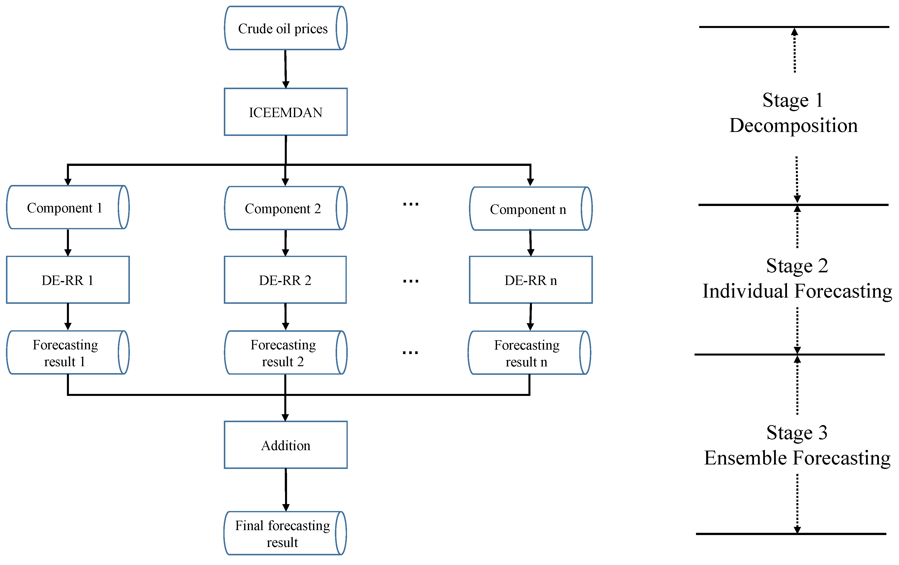
3.2. The Proposed ICEEMDAN-DE-RR Approach
- Stage 1:
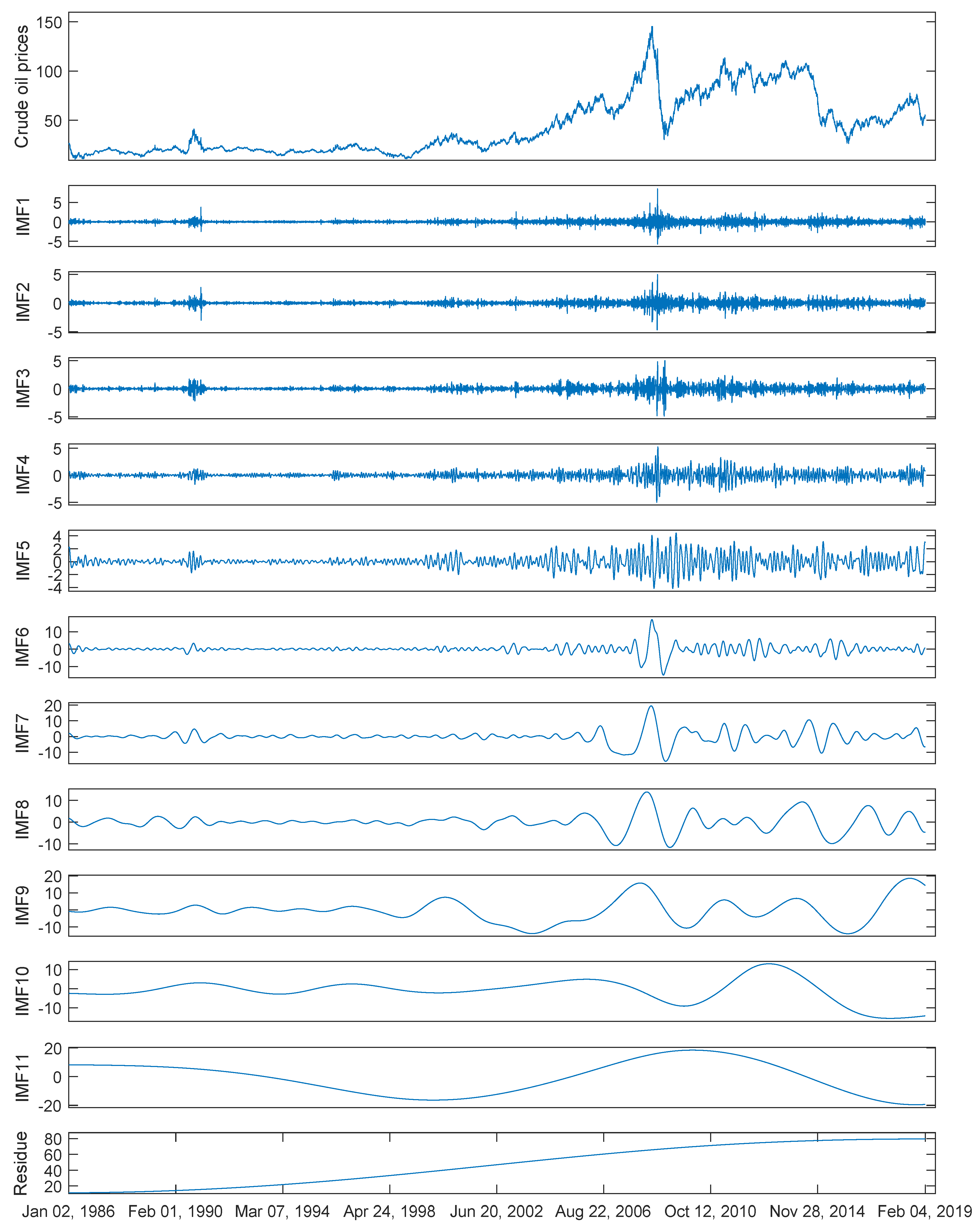
- Decomposition. The daily raw crude oil price series is decomposed into two groups of components: several IMFs and one residue.
- Stage 2:
- Individual forecasting. The data samples in each component are divided into training set, validation set, and test set. The training set and validation set are used to build RR models, and then the test set is applied to evaluate the models. For each model, we use DE to optimize the regularization item, corresponding kernel parameters, and possible weights.
- Stage 3:
- Ensemble forecasting. The individual forecasting results of all the components in Stage 2 are aggregated as the final forecasting results by addition.
4. Experimental Results and Comparative Analysis
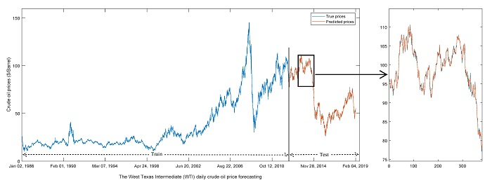
4.1. Data Description
4.2. Evaluation Criteria
4.3. Experimental Settings
4.4. Results and Analysis
4.4.1. Single Models
4.4.2. Ensemble Models
4.5. Discussion
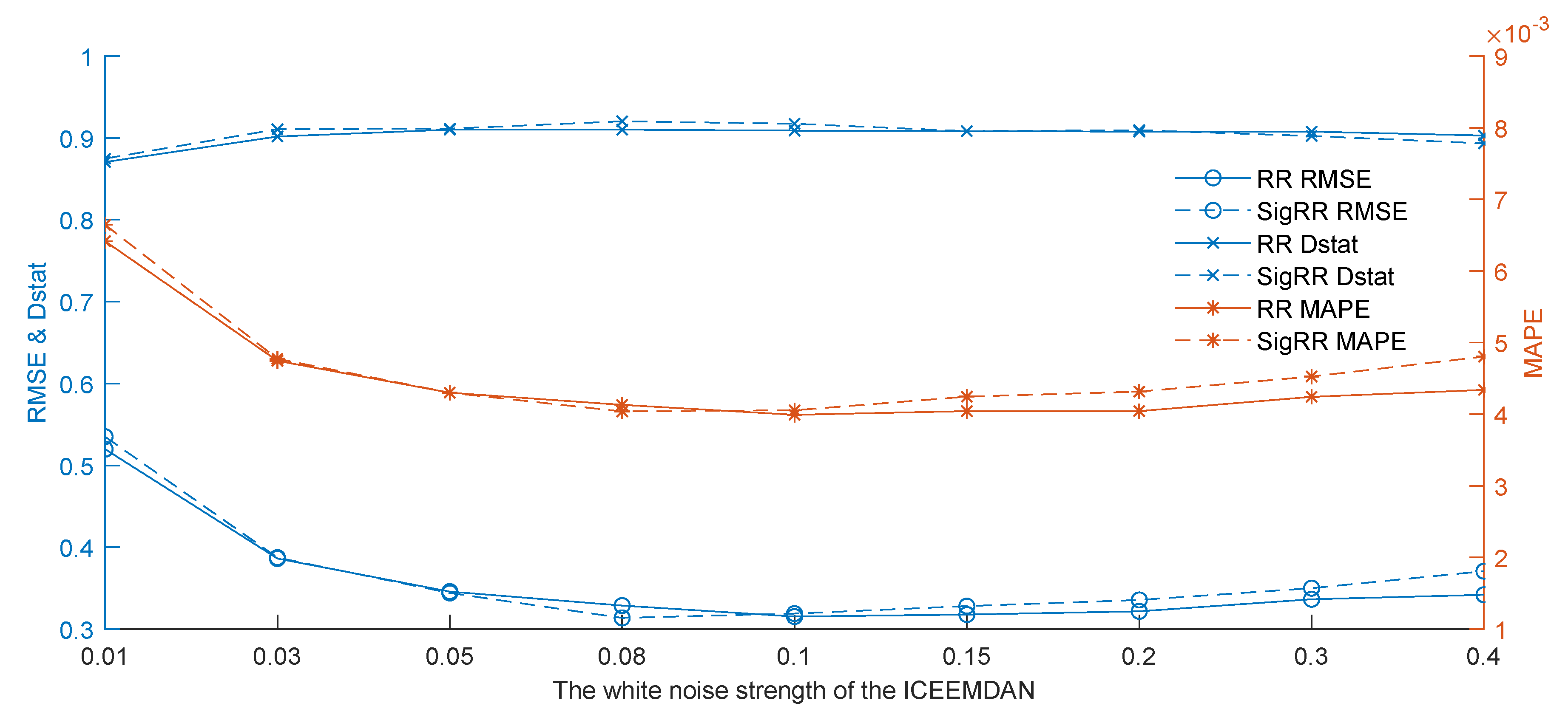
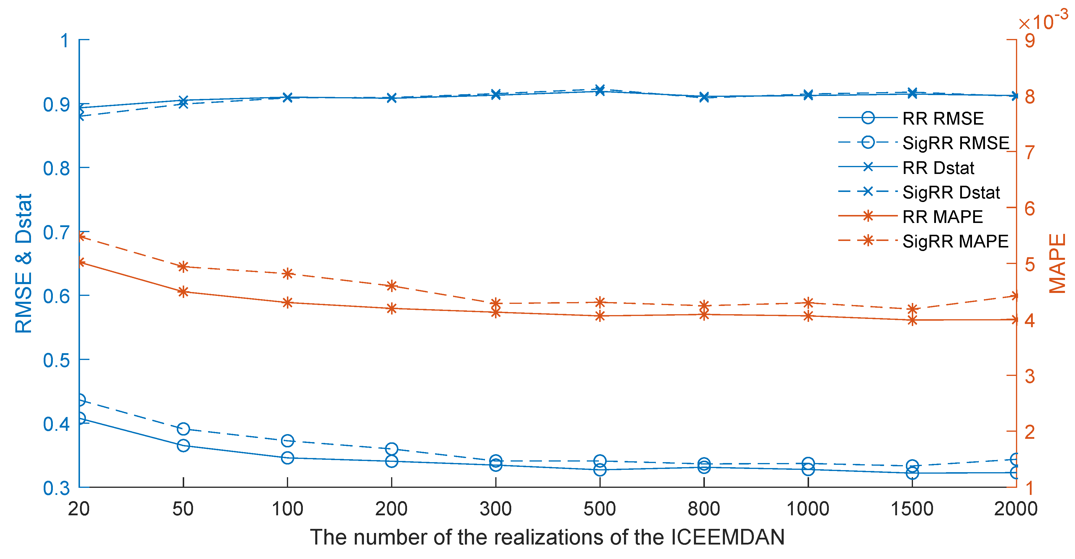
4.5.1. The Impact of the Parameter Settings of the ICEEMDAN
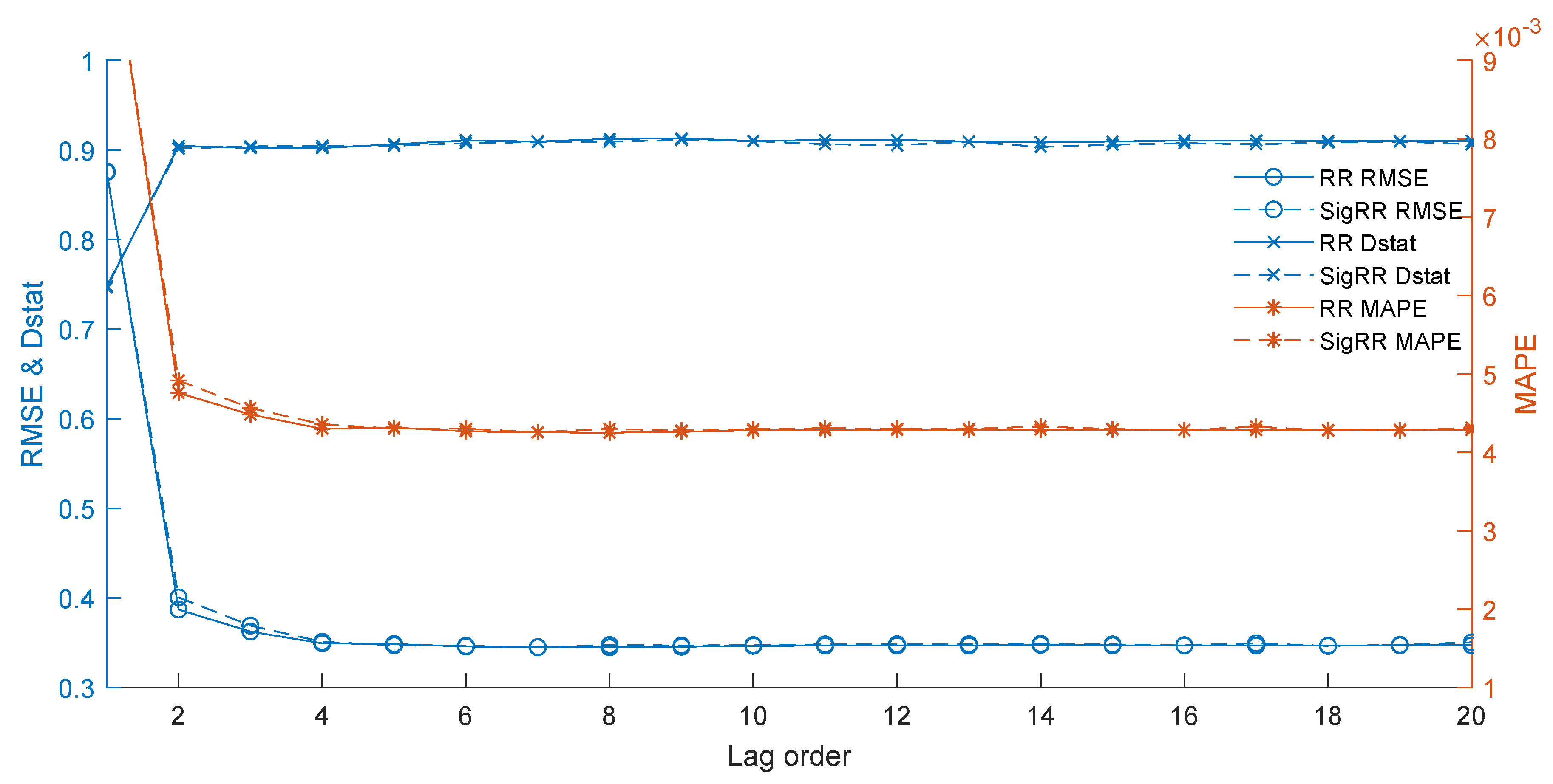
4.5.2. The Impact of the Lag Orders
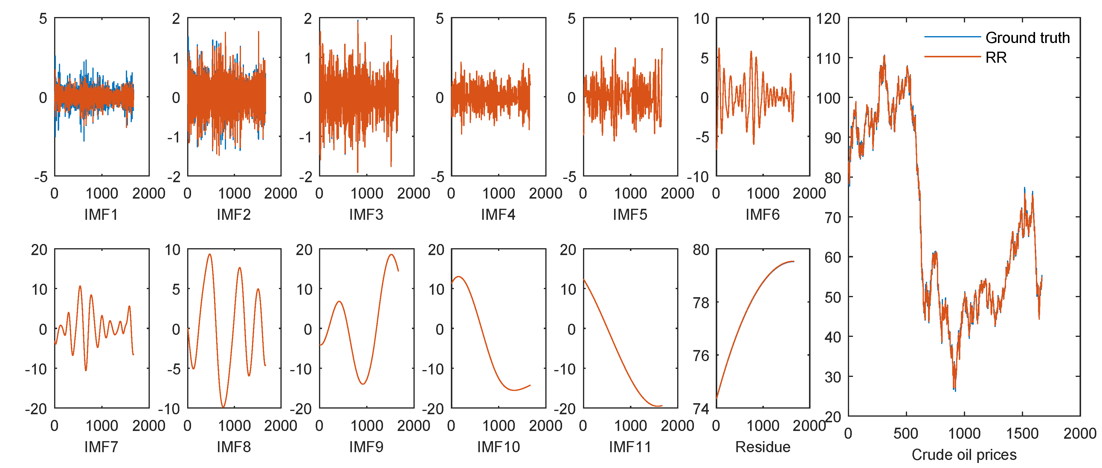
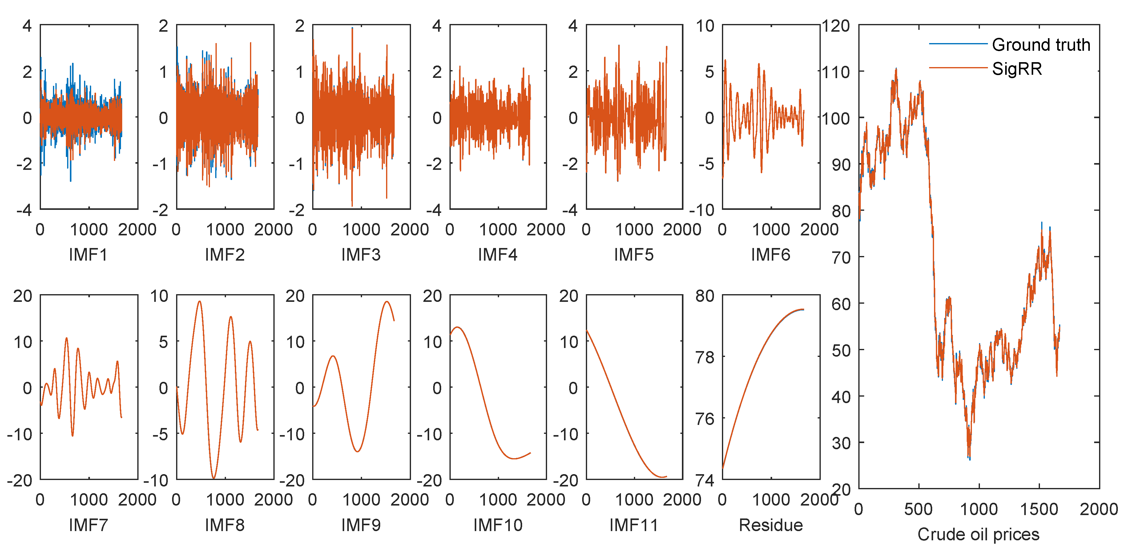
4.5.3. The Result of Each Individual Component
5. Summary and Conclusions
Author Contributions
Funding
Conflicts of Interest
References
- Miao, H.; Ramchander, S.; Wang, T.; Yang, D. Influential factors in crude oil price forecasting. Energy Econ. 2017, 68, 77–88. [Google Scholar] [CrossRef]
- Naderi, M.; Khamehchi, E.; Karimi, B. Novel statistical forecasting models for crude oil price, gas price, and interest rate based on meta-heuristic bat algorithm. J. Pet. Sci. Eng. 2019, 172, 13–22. [Google Scholar] [CrossRef]
- Ye, M.; Zyren, J.; Shore, J. A monthly crude oil spot price forecasting model using relative inventories. Int. J. Forecast. 2005, 21, 491–501. [Google Scholar] [CrossRef]
- Movagharnejad, K.; Mehdizadeh, B.; Banihashemi, M.; Kordkheili, M.S. Forecasting the differences between various commercial oil prices in the Persian Gulf region by neural network. Energy 2011, 36, 3979–3984. [Google Scholar] [CrossRef]
- Zhang, Y.; Ma, F.; Shi, B.; Huang, D. Forecasting the prices of crude oil: An iterated combination approach. Energy Econ. 2018, 70, 472–483. [Google Scholar] [CrossRef]
- Wen, F.; Gong, X.; Cai, S. Forecasting the volatility of crude oil futures using HAR-type models with structural breaks. Energy Econ. 2016, 59, 400–413. [Google Scholar] [CrossRef]
- Li, J.; Zhu, S.; Wu, Q. Monthly crude oil spot price forecasting using variational mode decomposition. Energy Econ. 2019, 83, 240–253. [Google Scholar] [CrossRef]
- Zhou, Y.; Li, T.; Shi, J.; Qian, Z. A CEEMDAN and XGBOOST-Based Approach to Forecast Crude Oil Prices. Complexity 2019, 2019, 4392785. [Google Scholar] [CrossRef]
- He, K.; Yu, L.; Lai, K.K. Crude oil price analysis and forecasting using wavelet decomposed ensemble model. Energy 2012, 46, 564–574. [Google Scholar] [CrossRef]
- Yu, L.; Dai, W.; Tang, L.; Wu, J. A hybrid grid-GA-based LSSVR learning paradigm for crude oil price forecasting. Neural Comput. Appl. 2016, 27, 2193–2215. [Google Scholar] [CrossRef]
- Tang, L.; Wu, Y.; Yu, L. A non-iterative decomposition-ensemble learning paradigm using RVFL network for crude oil price forecasting. Appl. Soft. Comput. 2018, 70, 1097–1108. [Google Scholar] [CrossRef]
- Yu, L.; Wang, S.; Lai, K.K. Forecasting crude oil price with an EMD-based neural network ensemble learning paradigm. Energy Econ. 2008, 30, 2623–2635. [Google Scholar] [CrossRef]
- Mirmirani, S.; Li, H.C. A comparison of VAR and neural networks with genetic algorithm in forecasting price of oil. Appl. Artif. Intell. Financ. Econ. 2004, 19, 203–223. [Google Scholar]
- Murat, A.; Tokat, E. Forecasting oil price movements with crack spread futures. Energy Econ. 2009, 31, 85–90. [Google Scholar] [CrossRef]
- Moshiri, S.; Foroutan, F. Forecasting nonlinear crude oil futures prices. Energy J. 2006, 27, 81–95. [Google Scholar] [CrossRef]
- Herrera, A.M.; Hu, L.; Pastor, D. Forecasting crude oil price volatility. Int. J. Forecast. 2018, 34, 622–635. [Google Scholar] [CrossRef]
- Nademi, A.; Nademi, Y. Forecasting crude oil prices by a semiparametric Markov switching model: OPEC, WTI, and Brent cases. Energy Econ. 2018, 74, 757–766. [Google Scholar] [CrossRef]
- Zhang, Y.J.; Yao, T.; He, L.Y.; Ripple, R. Volatility forecasting of crude oil market: Can the regime switching GARCH model beat the single-regime GARCH models? Int. Rev. Econ. Financ. 2019, 59, 302–317. [Google Scholar] [CrossRef]
- Lyocsa, S.; Molnar, P. Exploiting dependence: Day-ahead volatility forecasting for crude oil and natural gas exchange-traded funds. Energy 2018, 155, 462–473. [Google Scholar] [CrossRef]
- Lv, W. Does the OVX matter for volatility forecasting? Evidence from the crude oil market. Phys. A 2018, 492, 916–922. [Google Scholar] [CrossRef]
- Naser, H. Estimating and forecasting the real prices of crude oil: A data rich model using a dynamic model averaging (DMA) approach. Energy Econ. 2016, 56, 75–87. [Google Scholar] [CrossRef]
- Azevedo, V.G.; Campos, L.M.S. Combination of forecasts for the price of crude oil on the spot market. Int. J. Prod. Res. 2016, 54, 5219–5235. [Google Scholar] [CrossRef]
- Tang, L.; Dai, W.; Yu, L. A Novel CEEMD-Based EELM Ensemble Learning Paradigm for Crude Oil Price Forecasting. Int. J. Inf. Technol. Decis. Mak. 2015, 14, 141–169. [Google Scholar] [CrossRef]
- Tehrani, R.; Khodayar, F. A hybrid optimized artificial intelligent model to forecast crude oil using genetic algorithm. Afr. J. Bus. Manag. 2011, 5, 13130–13135. [Google Scholar] [CrossRef]
- Xiong, T.; Bao, Y.; Hu, Z. Beyond one-step-ahead forecasting: Evaluation of alternative multi-step-ahead forecasting models for crude oil prices. Energy Econ. 2013, 40, 405–415. [Google Scholar] [CrossRef]
- Barunik, J.; Malinska, B. Forecasting the term structure of crude oil futures prices with neural networks. Appl. Energy 2016, 164, 366–379. [Google Scholar] [CrossRef]
- Ding, Y. A novel decompose-ensemble methodology with AIC-ANN approach for crude oil forecasting. Energy 2018, 154, 328–336. [Google Scholar] [CrossRef]
- Fan, L.; Pan, S.; Li, Z.; Li, H. An ICA-based support vector regression scheme for forecasting crude oil prices. Technol. Forecast. Soc. Chang. 2016, 112, 245–253. [Google Scholar] [CrossRef]
- Yu, L.; Zhang, X.; Wang, S. Assessing Potentiality of Support Vector Machine Method in Crude Oil Price Forecasting. Eurasia J. Math. Sci. Technol. Educ. 2017, 13, 7893–7904. [Google Scholar] [CrossRef]
- Zhang, Y.; Zhang, J. Volatility forecasting of crude oil market: A new hybrid method. J. Forecast. 2018, 37, 781–789. [Google Scholar] [CrossRef]
- Li, T.; Hu, Z.; Jia, Y.; Wu, J.; Zhou, Y. Forecasting Crude Oil Prices Using Ensemble Empirical Mode Decomposition and Sparse Bayesian Learning. Energies 2018, 11, 1882. [Google Scholar] [CrossRef]
- Wu, J.; Chen, Y.; Zhou, T.; Li, T. An Adaptive Hybrid Learning Paradigm Integrating CEEMD, ARIMA and SBL for Crude Oil Price Forecasting. Energies 2019, 12, 1239. [Google Scholar] [CrossRef]
- Yu, L.; Dai, W.; Tang, L. A novel decomposition ensemble model with extended extreme learning machine for crude oil price forecasting. Eng. Appl. Artif. Intell. 2016, 47, 110–121. [Google Scholar] [CrossRef]
- Wang, J.; Athanasopoulos, G.; Hyndman, R.J.; Wang, S. Crude oil price forecasting based on internet concern using an extreme learning machine. Int. J. Forecast. 2018, 34, 665–677. [Google Scholar] [CrossRef]
- Wu, Y.X.; Wu, Q.B.; Zhu, J.Q. Improved EEMD-based crude oil price forecasting using LSTM networks. Phys. A 2019, 516, 114–124. [Google Scholar] [CrossRef]
- Li, T.; Zhou, M.; Guo, C.; Luo, M.; Wu, J.; Pan, F.; Tao, Q.; He, T. Forecasting Crude Oil Price Using EEMD and RVM with Adaptive PSO-Based Kernels. Energies 2016, 9, 1014. [Google Scholar] [CrossRef]
- Chiroma, H.; Abdul-kareem, S.; Noor, A.S.M.; Abubakar, A.I.; Safa, N.S.; Shuib, L.; Hamza, M.F.; Gital, A.Y.; Herawan, T. A Review on Artificial Intelligence Methodologies for the Forecasting of Crude Oil Price. Intell. Autom. Soft Comput. 2016, 22, 449–462. [Google Scholar] [CrossRef]
- Deng, W.; Zhang, S.; Zhao, H.; Yang, X. A Novel Fault Diagnosis Method Based on Integrating Empirical Wavelet Transform and Fuzzy Entropy for Motor Bearing. IEEE Access 2018, 6, 35042–35056. [Google Scholar] [CrossRef]
- Zhao, H.; Yao, R.; Xu, L.; Yuan, Y.; Li, G.; Deng, W. Study on a Novel Fault Damage Degree Identification Method Using High-Order Differential Mathematical Morphology Gradient Spectrum Entropy. Entropy 2018, 20, 682. [Google Scholar] [CrossRef]
- Bajaj, V.; Pachori, R.B. Classification of Seizure and Nonseizure EEG Signals Using Empirical Mode Decomposition. IEEE Trans. Inf. Technol. Biomed. 2012, 16, 1135–1142. [Google Scholar] [CrossRef] [PubMed]
- Li, T.; Zhou, M. ECG Classification Using Wavelet Packet Entropy and Random Forests. Entropy 2016, 18, 285. [Google Scholar] [CrossRef]
- Zhang, H.; Wang, X.; Cao, J.; Tang, M.; Guo, Y. A multivariate short-term traffic flow forecasting method based on wavelet analysis and seasonal time series. Appl. Intell. 2018, 48, 3827–3838. [Google Scholar] [CrossRef]
- Pannakkong, W.; Sriboonchitta, S.; Huynh, V.N. An Ensemble Model of Arima and Ann with Restricted Boltzmann Machine Based on Decomposition of Discrete Wavelet Transform for Time Series Forecasting. J. Syst. Sci. Syst. Eng. 2018, 27, 690–708. [Google Scholar] [CrossRef]
- Li, T.; Yang, M.; Wu, J.; Jing, X. A novel image encryption algorithm based on a fractional-order hyperchaotic system and DNA computing. Complexity 2017, 2017, 9010251. [Google Scholar] [CrossRef]
- Li, T.; Shi, J.; Li, X.; Wu, J.; Pan, F. Image encryption based on pixel-level diffusion with dynamic filtering and DNA-level permutation with 3D Latin cubes. Entropy 2019, 21, 319. [Google Scholar] [CrossRef]
- Li, X.; Xie, Z.; Wu, J.; Li, T. Image encryption based on dynamic filtering and bit cuboid operations. Complexity 2019, 2019, 7485621. [Google Scholar] [CrossRef]
- Ren, Y.; Suganthan, P.N.; Srikanth, N. A Novel Empirical Mode Decomposition with Support Vector Regression for Wind Speed Forecasting. IEEE Trans. Neural Netw. Learn. Syst. 2016, 27, 1793–1798. [Google Scholar] [CrossRef] [PubMed]
- Yang, Z.S.; Wang, J. A combination forecasting approach applied in multistep wind speed forecasting based on a data processing strategy and an optimized artificial intelligence algorithm. Appl. Energy 2018, 230, 1108–1125. [Google Scholar] [CrossRef]
- Abdoos, A.; Hemmati, M.; Abdoos, A.A. Short term load forecasting using a hybrid intelligent method. Knowl.-Based Syst. 2015, 76, 139–147. [Google Scholar] [CrossRef]
- Fan, G.F.; Peng, L.L.; Hong, W.C.; Sun, F. Electric load forecasting by the SVR model with differential empirical mode decomposition and auto regression. Neurocomputing 2016, 173, 958–970. [Google Scholar] [CrossRef]
- Qiu, X.H.; Ren, Y.; Suganthan, P.N.; Amaratunga, G.A.J. Empirical Mode Decomposition based ensemble deep learning for load demand time series forecasting. Appl. Soft. Comput. 2017, 54, 246–255. [Google Scholar] [CrossRef]
- Sun, W.; Zhang, C.C. Analysis and forecasting of the carbon price using multi resolution singular value decomposition and extreme learning machine optimized by adaptive whale optimization algorithm. Appl. Energy 2018, 231, 1354–1371. [Google Scholar] [CrossRef]
- Wang, D.Y.; Luo, H.Y.; Grunder, O.; Lin, Y.B.; Guo, H.X. Multi-step ahead electricity price forecasting using a hybrid model based on two-layer decomposition technique and BP neural network optimized by firefly algorithm. Appl. Energy 2017, 190, 390–407. [Google Scholar] [CrossRef]
- Yang, Z.S.; Wang, J. A hybrid forecasting approach applied in wind speed forecasting based on a data processing strategy and an optimized artificial intelligence algorithm. Energy 2018, 160, 87–100. [Google Scholar] [CrossRef]
- Huang, N.E.; Shen, Z.; Long, S.R. A new view of nonlinear water waves: the Hilbert Spectrum 1. Annu. Rev. Fluid Mech. 1999, 31, 417–457. [Google Scholar] [CrossRef]
- Wu, Z.; Huang, N.E. Ensemble empirical mode decomposition: A noise-assisted data analysis method. Adv. Adapt. Data Anal 2009, 1, 1–41. [Google Scholar] [CrossRef]
- Torres, M.E.; Colominas, M.A.; Schlotthauer, G.; Flandrin, P. A complete ensemble empirical mode decomposition with adaptive noise. In Proceedings of the 2011 IEEE international conference on acoustics, speech and signal processing (ICASSP), Prague, Czech Republic, 22–27 May 2011; pp. 4144–4147. [Google Scholar]
- Colominas, M.A.; Schlotthauer, G.; Torres, M.E. Improved complete ensemble EMD: A suitable tool for biomedical signal processing. Biomed. Signal Process. Control 2014, 14, 19–29. [Google Scholar] [CrossRef]
- Dai, S.; Niu, D.; Li, Y. Daily peak load forecasting based on complete ensemble empirical mode decomposition with adaptive noise and support vector machine optimized by modified grey Wolf optimization algorithm. Energies 2018, 11, 163. [Google Scholar] [CrossRef]
- Douak, F.; Melgani, F.; Benoudjit, N. Kernel ridge regression with active learning for wind speed prediction. Appl. Energy 2013, 103, 328–340. [Google Scholar] [CrossRef]
- Naik, J.; Satapathy, P.; Dash, P.K. Short-term wind speed and wind power prediction using hybrid empirical mode decomposition and kernel ridge regression. Appl. Soft. Comput. 2018, 70, 1167–1188. [Google Scholar] [CrossRef]
- Qian, C.; Breckon, T.P.; Li, H. Robust visual tracking via speedup multiple kernel ridge regression. J. Electron. Imaging 2015, 24, 053016. [Google Scholar] [CrossRef]
- Maalouf, M.; Homouz, D.; Abutayeh, M. Accurate Prediction of Preheat Temperature in Solar Flash Desalination Systems Using Kernel Ridge Regression. J. Energy Eng. 2016, 142, E4015017. [Google Scholar] [CrossRef]
- Naik, J.; Bisoi, R.; Dash, P.K. Prediction interval forecasting of wind speed and wind power using modes decomposition based low rank multi-kernel ridge regression. Renew. Energy 2018, 129, 357–383. [Google Scholar] [CrossRef]
- Kennedy, J. Particle swarm optimization. In Encyclopedia of Machine Learning; Springer: Berlin, Germany, 2010; pp. 760–766. [Google Scholar]
- Deng, W.; Zhao, H.; Yang, X.; Xiong, J.; Sun, M.; Li, B. Study on an improved adaptive PSO algorithm for solving multi-objective gate assignment. Appl. Soft. Comput. 2017, 59, 288–302. [Google Scholar] [CrossRef]
- Deng, W.; Yao, R.; Zhao, H.; Yang, X.; Li, G. A novel intelligent diagnosis method using optimal LS-SVM with improved PSO algorithm. Soft Comput. 2019, 23, 2445–2462. [Google Scholar] [CrossRef]
- Storn, R.; Price, K. Differential evolution—A simple and efficient heuristic for global optimization over continuous spaces. J. Glob. Optim. 1997, 11, 341–359. [Google Scholar] [CrossRef]
- Das, S.; Suganthan, P.N. Differential Evolution: A Survey of the State-of-the-Art. IEEE Trans. Evol. Comput. 2011, 15, 4–31. [Google Scholar] [CrossRef]
- Dorigo, M.; Blum, C. Ant colony optimization theory: A survey. Theor. Comput. Sci. 2005, 344, 243–278. [Google Scholar] [CrossRef]
- Deng, W.; Xu, J.; Zhao, H. An Improved Ant Colony Optimization Algorithm Based on Hybrid Strategies for Scheduling problem. IEEE Access 2019, 20281–20292. [Google Scholar] [CrossRef]
- Yu, X.; Liong, S.Y. Forecasting of hydrologic time series with ridge regression in feature space. J. Hydrol. 2007, 332, 290–302. [Google Scholar] [CrossRef]
- Ahn, J.J.; Byun, H.W.; Oh, K.J.; Kim, T.Y. Using ridge regression with genetic algorithm to enhance real estate appraisal forecasting. Expert Syst. Appl. 2012, 39, 8369–8379. [Google Scholar] [CrossRef]
- Zhang, S.; Hu, Q.; Xie, Z.; Mi, J. Kernel ridge regression for general noise model with its application. Neurocomputing 2015, 149, 836–846. [Google Scholar] [CrossRef]
- Saunders, C.; Gammerman, A.; Vovk, V. Ridge Regression Learning Algorithm in Dual Variables. In Proceedings of the Fifteenth International Conference on Machine Learning, Madison, WI, USA, 24–27 July 1998; Morgan Kaufmann Publishers Inc.: San Francisco, CA, USA, 1998; pp. 515–521. [Google Scholar]
- Maalouf, M.; Barsoum, Z. Failure strength prediction of aluminum spot-welded joints using kernel ridge regression. Int. J. Adv. Manuf. Technol. 2017, 91, 3717–3725. [Google Scholar] [CrossRef]
- Avron, H.; Clarkson, K.L.; Woodruff, D.P. Faster kernel ridge regression using sketching and preconditioning. SIAM J. Matrix Anal. Appl. 2017, 38, 1116–1138. [Google Scholar] [CrossRef]
- Diebold, F.; Mariano, R. Comparing predictive accuracy. J. Bus. Econ. Stat. 2002, 20, 134–144. [Google Scholar] [CrossRef]
- Sakamoto, Y.; Ishiguro, M.; Kitagawa, G. Akaike Information Criterion Statistics; Reidel, D., Ed.; Springer: Dordrecht, The Netherlands, 1986; Volume 81. [Google Scholar]


| Method | Description | Parameters |
|---|---|---|
| EEMD | Ensemble empirical mode decomposition | Noise standard deviation: 0.2; Number of realizations: 100. |
| ICEEMDAN | Improved complete EEMD with adaptive noise | Noise standard deviation: 0.05; Number of realizations: 500; Maximum number of sifting iterations allowed: 5000. |
| RR | Ridge Regression | : [0.001, 0.2]. |
| LinRR | RR with a linear kernel | : [0.001, 0.2]. |
| PolyRR | RR with a polynomial kernel | : [0.001, 0.2]; a: [0, 2]; b: [0, 10]; c: {1,2,3,4}. |
| SigRR | RR with a Sigmoid kernel | : [0.001, 0.2]; d: [0, 4]; e: [0, 8]. |
| RbfRR | RR with a radial basis functional kernel | : [0.001, 0.2]; f: . |
| MKRR | RR with multiple kernels as formulated in Equation (19) | : [0.001, 0.2]; : the same as the above single kernel; n: 20, number of the RBF kernels; : ; : . |
| LSSVR | Least square support vector regression with a RBF kernel | Regularization parameter: ; Width of the RBF kernel: . |
| BPNN | Back propagation neural network | Size of the hidden layer: {10, 20, 50, 100}; Maximum training epochs: {100, 1000, 10000}; Learning rate: {0.001, 0.01, 0.05, 0.1}. |
| ARIMA | Autoregressive integrated moving average | Akaike information criterion (AIC) to determine parameters (p-d-q) [79]. |
| DE | Differential Evolution | Population size: 20; Number of iterations: 40; Crossover probability: 0.2. |
| Horizon | Criterion | RR | LinRR | PolyRR | SigRR | RbfRR | MKRR | LSSVR | BPNN | ARIMA | RW |
|---|---|---|---|---|---|---|---|---|---|---|---|
| 1 | MAPE | 0.0154 | 0.0154 | 0.0154 | 0.0154 | 0.0156 | 0.0154 | 0.0154 | 0.0161 | 0.0157 | 0.0156 |
| RMSE | 1.2454 | 1.2462 | 1.2473 | 1.2483 | 1.2567 | 1.2472 | 1.2481 | 1.3050 | 1.2701 | 1.2700 | |
| Dstat | 0.5000 | 0.4940 | 0.5132 | 0.5156 | 0.5186 | 0.5162 | 0.5102 | 0.5132 | 0.4868 | 0.5054 | |
| 3 | MAPE | 0.0262 | 0.0263 | 0.0264 | 0.0264 | 0.0265 | 0.0263 | 0.0266 | 0.0264 | 0.0274 | 0.0272 |
| RMSE | 2.0627 | 2.0689 | 2.0708 | 2.0701 | 2.0754 | 2.0767 | 2.0801 | 2.0797 | 2.1713 | 2.1645 | |
| Dstat | 0.4988 | 0.4988 | 0.4964 | 0.4958 | 0.5000 | 0.5090 | 0.4952 | 0.4994 | 0.4982 | 0.4952 | |
| 6 | MAPE | 0.0377 | 0.0379 | 0.0381 | 0.0381 | 0.0381 | 0.0380 | 0.0379 | 0.0394 | 0.0408 | 0.0401 |
| RMSE | 2.8977 | 2.9101 | 2.9209 | 2.9208 | 2.9239 | 2.9149 | 2.9128 | 2.9943 | 3.1824 | 3.1195 | |
| Dstat | 0.4952 | 0.4958 | 0.4862 | 0.4898 | 0.4922 | 0.4964 | 0.4910 | 0.4976 | 0.4916 | 0.4928 |
| Horizon | Tested Model | LinRR | PolyRR | SigRR | RbfRR | MKRR | LSSVR | BPNN | ARIMA | RW |
|---|---|---|---|---|---|---|---|---|---|---|
| 1 | RR | −1.1025 (0.2704) | −0.7203 (0.4714) | −1.5290 (0.1265) | −2.0533 (0.0402) | −0.6405 (0.5219) | −1.3788 (0.1681) | −5.5601 (0.0000) | −3.4678 (0.0005) | −3.4585 (0.0004) |
| LinRR | −0.4701 (0.6383) | −1.3435 (0.1793) | −1.6807 (0.0930) | −0.3852 (0.7001) | −1.3221 (0.1863) | −5.6817 (0.0000) | −3.3577 (0.0008) | −3.2647 (0.0007) | ||
| PolyRR | −0.4864 (0.6268) | −1.3044 (0.1923) | 0.2103 (0.8334) | −0.4205 (0.6742) | −5.7019 (0.0000) | −2.8226 (0.0048) | −2.7642 (0.0000) | |||
| SigRR | −1.2372 (0.2162) | 0.5057 (0.6132) | 0.1453 (0.8845) | −5.7208 (0.0000) | −2.8937 (0.0039) | −2.3072 (0.0002) | ||||
| RbfRR | 1.3294 (0.1839) | 1.2083 (0.2271) | −3.4277 (0.0006) | −1.3067 (0.1915) | −1.2796 (0.0142) | |||||
| MKRR | −0.4335 (0.6647) | −5.7099 (0.0000) | −2.8012 (0.0052) | −2.7326 (0.0312) | ||||||
| LSSVR | −5.8110 (0.0000) | −2.8584 (0.0043) | −2.6057 (0.0147) | |||||||
| BPNN | 2.6579 (0.0079) | 2.1439 (0.0001) | ||||||||
| ARIMA | 0.0996 (0.1206) | |||||||||
| 3 | RR | −2.4997 (0.0125) | −1.6877 (0.0916) | −2.0321 (0.0423) | −2.8803 (0.0040) | −2.3015 (0.0215) | −3.2386 (0.0012) | −2.7039 (0.0069) | −5.6427 (0.0000) | −4.9664 (0.0000) |
| LinRR | −0.2930 (0.7696) | −0.2368 (0.8129) | −2.0401 (0.0415) | −1.0401 (0.2984) | −2.9172 (0.0036) | −1.3601 (0.1740) | −5.1351 (0.0000) | −5.1652 (0.0000) | ||
| PolyRR | 0.1966 (0.8442) | −0.6415 (0.5213) | −1.6590 (0.0973) | −1.1121 (0.2662) | −2.1367 (0.0328) | −4.6340 (0.0000) | −4.9189 (0.0000) | |||
| SigRR | −1.0601 (0.2893) | −1.6399 (0.1012) | −1.6464 (0.0999) | −1.8857 (0.0595) | −4.8619 (0.0000) | −4.6375 (0.0000) | ||||
| RbfRR | −0.1690 (0.8658) | −3.6421 (0.0003) | −0.5004 (0.6169) | −4.4865 (0.0000) | −4.4237 (0.0000) | |||||
| MKRR | −0.4004 (0.6889) | −0.5933 (0.5530) | −4.3286 (0.0000) | −3.3925 (0.0000) | ||||||
| LSSVR | 0.0403 (0.9679) | −4.2520 (0.0000) | −3.8976 (0.0000) | |||||||
| BPNN | −4.4861 (0.0000) | −4.3547 (0.0001) | ||||||||
| ARIMA | 0.7708 (0.1300) | |||||||||
| 6 | RR | −2.6901 (0.0072) | −3.0491 (0.0023) | −3.1495 (0.0017) | −3.2282 (0.0013) | −1.4575 (0.1452) | −2.4926 (0.0128) | −5.1039 (0.0000) | −7.6069 (0.0000) | −7.9403 (0.0000) |
| LinRR | −1.3345 (0.1822) | −1.2552 (0.2096) | −2.1339 (0.0330) | −0.3964 (0.6919) | −0.3807 (0.7035) | −4.2189 (0.0000) | −7.0961 (0.0000) | −6.8125 (0.0000) | ||
| PolyRR | 0.0718 (0.9428) | −0.6199 (0.5354) | 0.6465 (0.5180) | 2.4994 (0.0125) | −4.9939 (0.0000) | −6.4072 (0.0000) | −6.0013 (0.0000) | |||
| SigRR | −0.5182 (0.6044) | 0.6242 (0.5326) | 2.2295 (0.0259) | −5.2852 (0.0000) | −6.3341 (0.0000) | −6.1752 (0.0000) | ||||
| RbfRR | 0.8653 (0.3870) | 2.6871 (0.0073) | −4.0728 (0.0000) | −6.3042 (0.0000) | −6.4841 (0.0000) | |||||
| MKRR | 0.2139 (0.8307) | −4.9976 (0.0000) | −6.4398 (0.0000) | −5.8925 (0.0000) | ||||||
| LSSVR | −5.0705 (0.0000) | −6.6890 (0.0000) | −6.5482 (0.0001) | |||||||
| BPNN | −4.0592 (0.0001) | −3.7692 (0.0002) | ||||||||
| ARIMA | 0.7134 (0.2304) |
| Decomposition | Horizon | Criterion | RR | LinRR | PolyRR | SigRR | RbfRR | MKRR | LSSVR | BPNN | RW |
|---|---|---|---|---|---|---|---|---|---|---|---|
| EEMD | 1 | MAPE | 0.0084 | 0.0089 | 0.0084 | 0.0084 | 0.0088 | 0.0085 | 0.0090 | 0.0200 | 0.0186 |
| RMSE | 0.6401 | 0.6827 | 0.6399 | 0.6399 | 0.6799 | 0.6467 | 0.6805 | 1.6044 | 1.7455 | ||
| Dstat | 0.8213 | 0.8112 | 0.8231 | 0.8189 | 0.7980 | 0.8135 | 0.8076 | 0.7344 | 0.5084 | ||
| 3 | MAPE | 0.0096 | 0.0111 | 0.0097 | 0.0097 | 0.0107 | 0.0100 | 0.0118 | 0.0195 | 0.0296 | |
| RMSE | 0.7569 | 0.8702 | 0.7583 | 0.7560 | 0.8410 | 0.7803 | 0.9406 | 1.5599 | 2.5344 | ||
| Dstat | 0.7746 | 0.7314 | 0.7728 | 0.7794 | 0.7500 | 0.7710 | 0.7272 | 0.6847 | 0.5000 | ||
| 6 | MAPE | 0.0120 | 0.0146 | 0.0121 | 0.0122 | 0.0147 | 0.0122 | 0.0126 | 0.0210 | 0.0396 | |
| RMSE | 0.9440 | 1.1602 | 0.9547 | 0.9704 | 1.1560 | 0.9666 | 0.9896 | 1.6297 | 3.1068 | ||
| Dstat | 0.7146 | 0.6607 | 0.7140 | 0.7002 | 0.6625 | 0.7290 | 0.6924 | 0.6265 | 0.4976 | ||
| ICEEMDAN | 1 | MAPE | 0.0043 | 0.0050 | 0.0043 | 0.0043 | 0.0048 | 0.0043 | 0.0044 | 0.0051 | 0.0175 |
| RMSE | 0.3458 | 0.4039 | 0.3469 | 0.3441 | 0.3901 | 0.3505 | 0.3528 | 0.3964 | 1.6209 | ||
| Dstat | 0.9101 | 0.8939 | 0.9101 | 0.9113 | 0.8975 | 0.9083 | 0.9071 | 0.8945 | 0.5228 | ||
| 3 | MAPE | 0.0073 | 0.0089 | 0.0074 | 0.0076 | 0.0087 | 0.0074 | 0.0075 | 0.0092 | 0.0286 | |
| RMSE | 0.5926 | 0.7170 | 0.5953 | 0.6067 | 0.7001 | 0.5984 | 0.6044 | 0.7022 | 2.4296 | ||
| Dstat | 0.8453 | 0.8040 | 0.8399 | 0.8417 | 0.8124 | 0.8393 | 0.8333 | 0.8100 | 0.4862 | ||
| 6 | MAPE | 0.0102 | 0.0138 | 0.0102 | 0.0107 | 0.0130 | 0.0103 | 0.0104 | 0.0187 | 0.0400 | |
| RMSE | 0.8027 | 1.0977 | 0.8100 | 0.8513 | 1.0276 | 0.8137 | 0.8236 | 1.3531 | 3.1926 | ||
| Dstat | 0.7590 | 0.6661 | 0.7584 | 0.7530 | 0.6847 | 0.7626 | 0.7578 | 0.6865 | 0.4982 |
| Horizon | Decomposition | Tested Model | ICEEMDAN | EEMD | ||||||||||||||||
|---|---|---|---|---|---|---|---|---|---|---|---|---|---|---|---|---|---|---|---|---|
| LinRR | PolyRR | SigRR | RbfRR | MKRR | LSSVR | BPNN | RW | RR | LinRR | PolyRR | SigRR | RbfRR | MKRR | LSSVR | BPNN | RW | ||||
| 1 | ICEEMDAN | RR | −7.6331 (0.0000) | −0.6142 (0.5392) | 0.9695 (0.3324) | −7.5172 (0.0000) | −1.9834 (0.0475) | −3.5554 (0.0004) | −12.8611 (0.0000) | −5.5386 (0.0000) | −21.3654 (0.0000) | −22.2857 (0.0000) | −21.2054 (0.0000) | −21.2416 (0.0000) | −21.3583 (0.0000) | −20.9534 (0.0000) | −22.0337 (0.0000) | −16.7261 (0.0000) | −4.0125 (0.0001) | |
| LinRR | 8.0753 (0.0000) | 7.8183 (0.0000) | 1.8874 (0.0593) | 6.9073 (0.0000) | 6.8284 (0.0000) | 0.9153 (0.3602) | −5.4460 (0.0000) | −17.1007 (0.0000) | −19.9938 (0.0000) | −17.0228 (0.0000) | −17.1490 (0.0000) | −18.1073 (0.0000) | −17.0138 (0.0000) | −18.4270 (0.0000) | −16.4052 (0.0000) | −3.9545 (0.0001) | ||||
| PolyRR | 2.1682 (0.0303) | −7.7155 (0.0000) | −1.7738 (0.0763) | −3.6728 (0.0002) | −12.0394 (0.0000) | −5.5375 (0.0000) | −21.3854 (0.0000) | −22.4548 (0.0000) | −21.3348 (0.0000) | −21.3959 (0.0000) | −21.4127 (0.0000) | −21.0541 (0.0000) | −22.1490 (0.0000) | −16.7245 (0.0000) | −4.0116 (0.0001) | |||||
| SigRR | −8.3841 (0.0000) | −2.7328 (0.0063) | −5.2931 (0.0000) | −12.1439 (0.0000) | −5.5416 (0.0000) | −21.3483 (0.0000) | −22.3840 (0.0000) | −21.2987 (0.0000) | −21.3724 (0.0000) | −21.5018 (0.0000) | −21.0097 (0.0000) | −22.1334 (0.0000) | −16.7370 (0.0000) | −4.0142 (0.0001) | ||||||
| RbfRR | 6.1499 (0.0000) | 6.7789 (0.0000) | −0.8816 (0.3781) | −5.4706 (0.0000) | −18.2902 (0.0000) | −20.4238 (0.0000) | −18.2305 (0.0000) | −18.4002 (0.0000) | −20.0042 (0.0000) | −18.1252 (0.0000) | −19.5005 (0.0000) | −16.5070 (0.0000) | −3.9687 (0.0001) | |||||||
| MKRR | −0.7986 (0.4246) | −11.7816 (0.0000) | −5.5313 (0.0000) | −21.1164 (0.0000) | −22.0611 (0.0000) | −21.0784 (0.0000) | −21.0921 (0.0000) | −20.9704 (0.0000) | −20.7933 (0.0000) | −21.8257 (0.0000) | −16.7113 (0.0000) | −4.0080 (0.0001) | ||||||||
| LSSVR | −10.4989 (0.0000) | −5.5281 (0.0000) | −20.9187 (0.0000) | −22.0006 (0.0000) | −20.8537 (0.0000) | −20.9486 (0.0000) | −21.1186 (0.0000) | −20.6389 (0.0000) | −21.8183 (0.0000) | −16.6977 (0.0000) | −4.0058 (0.0001) | |||||||||
| BPNN | −5.4562 (0.0000) | −17.9970 (0.0000) | −19.3554 (0.0000) | −17.9211 (0.0000) | −17.9391 (0.0000) | −18.2960 (0.0000) | −17.8094 (0.0000) | −19.1642 (0.0000) | −16.4971 (0.0000) | −3.9608 (0.0001) | ||||||||||
| RW | 4.8947 (0.0000) | 4.7746 (0.0000) | 4.8956 (0.0000) | 4.8959 (0.0000) | 4.7796 (0.0000) | 4.8761 (0.0000) | 4.7762 (0.0000) | 0.1120 (0.9109) | −0.4916 (0.6231) | |||||||||||
| EEMD | RR | −5.9878 (0.0000) | 0.0981 (0.9218) | 0.0921 (0.9266) | −5.8039 (0.0000) | −1.9935 (0.0464) | −7.2864 (0.0000) | −14.8109 (0.0000) | −3.6137 (0.0003) | |||||||||||
| LinRR | 5.8354 (0.0000) | 6.0493 (0.0000) | 0.3207 (0.7485) | 4.6149 (0.0000) | 0.2467 (0.8052) | −14.3910 (0.0000) | −3.5387 (0.0004) | |||||||||||||
| PolyRR | 0.0195 (0.9844) | −5.7741 (0.0000) | −2.2603 (0.0239) | −7.7598 (0.0000) | −14.8346 (0.0000) | −3.6141 (0.0003) | ||||||||||||||
| SigRR | −5.8048 (0.0000) | −2.4071 (0.0162) | −8.0538 (0.0000) | −14.8512 (0.0000) | −3.6144 (0.0003) | |||||||||||||||
| RbfRR | 4.6221 (0.0000) | −0.1080 (0.9140) | −14.4850 (0.0000) | −3.5431 (0.0004) | ||||||||||||||||
| MKRR | −7.2584 (0.0000) | −14.8197 (0.0000) | −3.6027 (0.0003) | |||||||||||||||||
| LSSVR | −14.5725 (0.0000) | −3.5415 (0.0004) | ||||||||||||||||||
| BPNN | −0.6384 (0.5233) | |||||||||||||||||||
| 3 | ICEEMDAN | RR | −9.9325 (0.0000) | −1.4417 (0.1496) | −3.7347 (0.0002) | −9.4380 (0.0000) | −2.4333 (0.0151) | −4.2254 (0.0000) | −13.4240 (0.0000) | −8.2617 (0.0000) | −12.9322 (0.0000) | −15.5357 (0.0000) | −13.0108 (0.0000) | −12.8337 (0.0000) | −14.9738 (0.0000) | −13.9333 (0.0000) | −16.8289 (0.0000) | −14.1737 (0.0000) | −8.1352 (0.0000) | |
| LinRR | 10.0119 (0.0000) | 9.7840 (0.0000) | 1.8443 (0.0653) | 9.5078 (0.0000) | 9.0895 (0.0000) | 1.0852 (0.2780) | −8.0440 (0.0000) | −2.6337 (0.0085) | −12.5877 (0.0000) | −2.7454 (0.0061) | −2.6451 (0.0082) | −8.2937 (0.0000) | −4.0327 (0.0001) | −10.8639 (0.0000) | −13.0047 (0.0000) | −7.9386 (0.0000) | ||||
| PolyRR | −4.4570 (0.0000) | −9.4540 (0.0000) | −1.1594 (0.2465) | −3.0217 (0.0026) | −13.1060 (0.0000) | −8.2580 (0.0000) | −12.5752 (0.0000) | −15.5953 (0.0000) | −12.7567 (0.0000) | −12.6621 (0.0000) | −14.8334 (0.0000) | −13.6041 (0.0000) | −16.7324 (0.0000) | −14.1551 (0.0000) | −8.1320 (0.0000) | |||||
| SigRR | −9.3379 (0.0000) | 1.9688 (0.0491) | 0.5195 (0.6035) | −10.9649 (0.0000) | −8.2399 (0.0000) | −11.3756 (0.0000) | −15.2838 (0.0000) | −11.5825 (0.0000) | −11.6158 (0.0000) | −14.3842 (0.0000) | −12.4692 (0.0000) | −16.2315 (0.0000) | −14.0525 (0.0000) | −8.1157 (0.0000) | ||||||
| RbfRR | 8.7712 (0.0000) | 8.8140 (0.0000) | −0.1757 (0.8605) | −8.0736 (0.0000) | −3.7902 (0.0002) | −11.6173 (0.0000) | −3.9565 (0.0001) | −3.9195 (0.0001) | −11.1280 (0.0000) | −5.2578 (0.0000) | −11.7123 (0.0000) | −13.2845 (0.0000) | −7.9644 (0.0000) | |||||||
| MKRR | −1.6406 (0.1011) | −12.7449 (0.0000) | −8.2505 (0.0000) | −12.6415 (0.0000) | −15.4153 (0.0000) | −12.7391 (0.0000) | −12.5443 (0.0000) | −14.6474 (0.0000) | −13.6362 (0.0000) | −16.5479 (0.0000) | −14.1136 (0.0000) | −8.1265 (0.0000) | ||||||||
| LSSVR | −13.4650 (0.0000) | −8.2427 (0.0000) | −11.9772 (0.0000) | −14.9897 (0.0000) | −12.1661 (0.0000) | −12.0859 (0.0000) | −14.6889 (0.0000) | −13.4358 (0.0000) | −16.4904 (0.0000) | −14.0859 (0.0000) | −8.1157 (0.0000) | |||||||||
| BPNN | −8.0500 (0.0000) | −3.9068 (0.0001) | −9.2782 (0.0000) | −4.1170 (0.0000) | −3.9602 (0.0001) | −8.0803 (0.0000) | −5.6840 (0.0000) | −11.3597 (0.0000) | −13.3170 (0.0000) | −7.9423 (0.0000) | ||||||||||
| RW | 7.9299 (0.0000) | 7.7031 (0.0000) | 7.9259 (0.0000) | 7.9322 (0.0000) | 7.7496 (0.0000) | 7.8725 (0.0000) | 7.4621 (0.0000) | 5.0472 (0.0000) | −0.5382 (0.5905) | |||||||||||
| EEMD | RR | −8.0803 (0.0000) | −0.6800 (0.4966) | 0.2481 (0.8041) | −7.6514 (0.0000) | −4.8069 (0.0000) | −12.0032 (0.0000) | −12.7901 (0.0000) | −7.8385 (0.0000) | |||||||||||
| LinRR | 7.9869 (0.0000) | 8.2376 (0.0000) | 2.2903 (0.0221) | 5.9929 (0.0000) | −3.7962 (0.0002) | −11.4198 (0.0000) | −7.6264 (0.0000) | |||||||||||||
| PolyRR | 1.1239 (0.2612) | −7.6591 (0.0000) | −4.7817 (0.0000) | −11.8134 (0.0000) | −12.8335 (0.0000) | −7.8359 (0.0000) | ||||||||||||||
| SigRR | −8.2382 (0.0000) | −4.8751 (0.0000) | −12.0577 (0.0000) | −12.8268 (0.0000) | −7.8411 (0.0000) | |||||||||||||||
| RbfRR | 5.3608 (0.0000) | −7.2419 (0.0000) | −11.9950 (0.0000) | −7.6714 (0.0000) | ||||||||||||||||
| MKRR | −10.3296 (0.0000) | −12.6336 (0.0000) | −7.7891 (0.0000) | |||||||||||||||||
| LSSVR | −10.7944 (0.0000) | −7.4217 (0.0000) | ||||||||||||||||||
| BPNN | −5.2626 (0.0000) | |||||||||||||||||||
| 6 | ICEEMDAN | RR | −13.9660 (0.0000) | −2.1767 (0.0296) | −6.0937 (0.0000) | −12.9968 (0.0000) | −2.4287 (0.0153) | −4.9536 (0.0000) | −22.6250 (0.0000) | −14.1579 (0.0000) | −12.3204 (0.0000) | −15.3905 (0.0000) | −12.0345 (0.0000) | −12.7060 (0.0000) | −15.1929 (0.0000) | −12.4624 (0.0000) | −13.2884 (0.0000) | −19.3882 (0.0000) | −17.6734 (0.0000) | |
| LinRR | 14.3951 (0.0000) | 14.3875 (0.0000) | 4.9217 (0.0000) | 13.1664 (0.0000) | 13.1583 (0.0000) | −9.0778 (0.0000) | −13.5116 (0.0000) | 7.7778 (0.0000) | −4.3984 (0.0000) | 7.4146 (0.0000) | 6.9775 (0.0000) | −3.0020 (0.0027) | 6.0234 (0.0000) | 5.4957 (0.0000) | −13.2753 (0.0000) | −16.9797 (0.0000) | ||||
| PolyRR | −7.2407 (0.0000) | −13.3457 (0.0000) | −0.7001 (0.4840) | −2.9388 (0.0033) | −22.1291 (0.0000) | −14.1522 (0.0000) | −11.6702 (0.0000) | −15.6854 (0.0000) | −11.7628 (0.0000) | −12.7550 (0.0000) | −15.3002 (0.0000) | −11.7487 (0.0000) | −13.1322 (0.0000) | −19.3071 (0.0000) | −17.6775 (0.0000) | |||||
| SigRR | −12.8356 (0.0000) | 4.1760 (0.0000) | 3.6412 (0.0003) | −20.1380 (0.0000) | −14.0771 (0.0000) | −7.3939 (0.0000) | −14.8116 (0.0000) | −8.1197 (0.0000) | −9.6893 (0.0000) | −14.2892 (0.0000) | −7.9142 (0.0000) | −10.1005 (0.0000) | −18.4915 (0.0000) | −17.5994 (0.0000) | ||||||
| RbfRR | 11.8646 (0.0000) | 12.5228 (0.0000) | −12.1621 (0.0000) | −13.6712 (0.0000) | 5.1460 (0.0000) | −6.9781 (0.0000) | 4.6379 (0.0000) | 3.9114 (0.0001) | −9.3717 (0.0000) | 3.4358 (0.0006) | 2.4569 (0.0141) | −14.7236 (0.0000) | −17.1397 (0.0000) | |||||||
| MKRR | −1.5720 (0.1161) | −22.1601 (0.0000) | −14.1246 (0.0000) | −10.9045 (0.0000) | −14.7753 (0.0000) | −10.8633 (0.0000) | −11.5082 (0.0000) | −14.4164 (0.0000) | −11.3219 (0.0000) | −12.0115 (0.0000) | −19.2344 (0.0000) | −17.6322 (0.0000) | ||||||||
| LSSVR | −22.0285 (0.0000) | −14.1061 (0.0000) | −10.1588 (0.0000) | −14.5608 (0.0000) | −10.2971 (0.0000) | −11.2871 (0.0000) | −14.9082 (0.0000) | −10.9314 (0.0000) | −12.6866 (0.0000) | −18.7911 (0.0000) | −17.6113 (0.0000) | |||||||||
| BPNN | −12.2861 (0.0000) | 16.3390 (0.0000) | 6.6381 (0.0000) | 16.0747 (0.0000) | 15.2332 (0.0000) | 6.7072 (0.0000) | 16.0034 (0.0000) | 14.0536 (0.0000) | −7.3185 (0.0000) | −15.2268 (0.0000) | ||||||||||
| RW | 13.8085 (0.0000) | 13.2857 (0.0000) | 13.7910 (0.0000) | 13.7611 (0.0000) | 13.2775 (0.0000) | 13.7266 (0.0000) | 13.6873 (0.0000) | 11.0380 (0.0000) | 0.7513 (0.4526) | |||||||||||
| EEMD | RR | −11.9133 (0.0000) | −2.8917 (0.0039) | −5.0101 (0.0000) | −11.8544 (0.0000) | −3.3420 (0.0009) | −7.1119 (0.0000) | −17.4323 (0.0000) | −17.2382 (0.0000) | |||||||||||
| LinRR | 11.6342 (0.0000) | 11.3981 (0.0000) | 0.2374 (0.8124) | 9.5491 (0.0000) | 9.4853 (0.0000) | −12.3880 (0.0000) | −16.6841 (0.0000) | |||||||||||||
| PolyRR | −4.2271 (0.0000) | −11.7039 (0.0000) | −1.5927 (0.1114) | −5.6236 (0.0000) | −17.1205 (0.0000) | −17.2187 (0.0000) | ||||||||||||||
| SigRR | −11.6910 (0.0000) | 0.4412 (0.6591) | −3.2085 (0.0014) | −16.7302 (0.0000) | −17.1929 (0.0000) | |||||||||||||||
| RbfRR | 9.9300 (0.0000) | 11.0223 (0.0000) | −12.7276 (0.0000) | −16.6240 (0.0000) | ||||||||||||||||
| MKRR | −2.6530 (0.0081) | −16.3767 (0.0000) | −17.1081 (0.0000) | |||||||||||||||||
| LSSVR | −16.6247 (0.0000) | −17.0843 (0.0000) | ||||||||||||||||||
| BPNN | −13.4903 (0.0000) | |||||||||||||||||||
© 2019 by the authors. Licensee MDPI, Basel, Switzerland. This article is an open access article distributed under the terms and conditions of the Creative Commons Attribution (CC BY) license (http://creativecommons.org/licenses/by/4.0/).
Share and Cite
Li, T.; Zhou, Y.; Li, X.; Wu, J.; He, T. Forecasting Daily Crude Oil Prices Using Improved CEEMDAN and Ridge Regression-Based Predictors. Energies 2019, 12, 3603. https://doi.org/10.3390/en12193603
Li T, Zhou Y, Li X, Wu J, He T. Forecasting Daily Crude Oil Prices Using Improved CEEMDAN and Ridge Regression-Based Predictors. Energies. 2019; 12(19):3603. https://doi.org/10.3390/en12193603
Chicago/Turabian StyleLi, Taiyong, Yingrui Zhou, Xinsheng Li, Jiang Wu, and Ting He. 2019. "Forecasting Daily Crude Oil Prices Using Improved CEEMDAN and Ridge Regression-Based Predictors" Energies 12, no. 19: 3603. https://doi.org/10.3390/en12193603
APA StyleLi, T., Zhou, Y., Li, X., Wu, J., & He, T. (2019). Forecasting Daily Crude Oil Prices Using Improved CEEMDAN and Ridge Regression-Based Predictors. Energies, 12(19), 3603. https://doi.org/10.3390/en12193603