Cost Forecasting Model of Transformer Substation Projects Based on Data Inconsistency Rate and Modified Deep Convolutional Neural Network

Abstract

Precise and steady substation project cost forecasting is of great significance to guarantee the economic construction and valid administration of electric power engineering. This paper develops a novel hybrid approach for cost forecasting based on a data inconsistency rate (DIR), a modified fruit fly optimization algorithm (MFOA) and a deep convolutional neural network (DCNN). Firstly, the DIR integrated with the MFOA is adopted for input feature selection. Simultaneously, the MFOA is utilized to realize parameter optimization in the DCNN. The effectiveness of the MFOA–DIR–DCNN has been validated by a case study that selects 128 substation projects in different regions for training and testing. The modeling results demonstrate that this established approach is better than the contrast methods with regard to forecasting accuracy and robustness. Thus, the developed technique is feasible for the cost prediction of substation projects in various voltage levels.

1. Introduction

The inadequate management and supervision of substation projects tend to bring about high cost, which has critical effects on the economy and sustainability of power engineering. Thus, cost prediction is of great importance for expense saving [1]. However, the comparable projects are hard to collect due to limited engineering in the same period as well as various influential factors such as the overall plan of the power grid, total capacity, terrain features, design and construction level, and local economy [2]. Along with the less sample data, the difficulty of cost forecasting for substation projects has been increased. Therefore, it is of great significance for the sustainability of electric power engineering investment to study and construct the substation cost forecasting model and accurately forecast the substation cost.

Nowadays, many scholars have published their momentous work to handle the cost forecasting of engineering, but few studies have focused on substation projects. The approaches in regard to engineering cost prediction are primarily separated into two kinds—traditional prediction methods and intelligent algorithms. Traditional forecasting techniques primarily consist of time series [3], grey prediction [4], regression analysis [5] and so on. Reference [3] designed a time series prediction model for engineering cost based on bills of quantities and evaluation. The results indicated that this proposed model controlled the error range within 5%. Reference [4] put forward an improved grey forecasting method optimized by a time response function to predict main construction cost indicators in power projects, where the constant C was determined through the minimum Euclidean distance of an original series and constraints of simulation values. In reference [6], a forecasting technique grounded on multiple structure integral linear regression was established in line with the characteristics of engineering cost composition. Principal component analysis was introduced here to address the multicollinearity. In spite of their mature theories and simple calculations, the defects of these methods, including narrow application scope and unideal forecasting accuracy, cannot be ignored.

With the burgeoning development of artificial intelligence, the application of intelligent algorithms in the cost prediction of substation projects is of great significance. This kind of model is chiefly composed of artificial neural networks (ANNs) and a support vector machine (SVM) [6], wherein some ANNs are applicable to forecasting fields including a back propagation neural network (BPNN), an extreme learning machine (ELM), a radial basis function neural network (RBFNN), and a general regression neural network (GRNN) [7]. Reference [8] executed a three-layer BPNN to forecast the cost of a transmission line project where the related influential factors were taken as the input. The model was validated on the foundation of actual data. Reference [9] put up with an ELM-based approach for medium and long term electricity demand prediction with the target of a low carbon economy. Reference [10] evaluated the effectiveness of a BPNN and a RBFNN for engineering cost prediction. The case study indicated that the RBFNN had a better performance in terms of forecasting accuracy. In literature [11], a hybrid model which combined a GRNN with a fruit fly optimization algorithm (FOA) was utilized in wind speed prediction, and good prediction results were obtained. Nevertheless, the defects of slow convergence and getting stuck in local best in a BPNN brought about a decrease of forecasting accuracy. To this end, an SVM was applied to refrain from network structure selection and mitigate the premature convergence to local optimization in engineering cost prediction [12]. Reference [13] investigated an SVM integrated with adaptive particle swarm optimization (APSO) to forecast the cost of a practical substation project. In reference [14], a cuckoo search algorithm (CS) was introduced to optimize the parameters in an SVM. The results showed that the forecasting precision was obviously enhanced. Compared with a BPNN, the application of an SVM can achieve better performance in cost prediction, but the transformation that converts the solution into a quadratic programming problem by the use of a kernel function in an SVM resulted in the decrease of efficiency and precision [15]. The aforementioned approaches belong to shallow learning algorithms, whose ability to cope with complex function problems is limited. In addition, these models cannot fully reflect information features in virtue of prior knowledge. Hence, some scholars tried to develop a deep neural network (DNN) for prediction [16].

The real powerful computing capability of neural networks has been brought into play since the creation of a DNN with “multi-layer structure and learning ability layer by layer” by Professor Hinton, University of Toronto in Canada in 2006. The DNN has aroused great concern in both academia and industry and has become a hot tool for data analysis in the big data era [17]. Additionally, this technique has made breakthroughs in the fields of signal recognition, natural language processing, and so on; it has also kept updating all kinds of records with amazing speed in diverse application areas [18]. In 2012, Krizhevsky et al. [19] put forward the concept of depth into traditional a convolutional neural network (CNN) and proposed a deep convolutional neural network (DCNN). The DCNN, as the first approach that successfully trains multi-layer networks, has been widely used owing to self-study of data characteristics [20]. Thereinto, the CNN model realizes the optimization of a neural network structure by self-convolution for local features, weight sharing, subsampling and multiple perception layers. Additionally, the CNN technique not only reduces the number of neurons and weights but also uses pooling operation to make input features invariable in displacement, scaling and distortion, which contributes to the improvement of accuracy and robustness for network training [21]. The DCNN has been employed in the area of prediction [22,23,24,25]. For instance, an original hybrid model on the basis of the DCNN was built to forecast the deterministic photovoltaic power in reference [22], where the DCNN was applied to nonlinear feature and invariant structure extraction presented in every frequency. The computing results indicate that the novel models can improve forecasting precision with respect to seasons along with various prediction horizons in contrast with conventional forecasting approaches. In reference [24], the DCNN integrated with a concretely ordered feature came up for the intraday direction forecasting of Borsa Istanbul 100 stocks. The results displayed that this established classifier is superior to logistic regression and the CNN in use of randomly ordered features. Thus, for the purpose of training time and model complexity reduction, feature selection models can be employed.

Considering the influence of parameter selection on prediction performance of the DCNN, it is indispensable to select a proper intelligent algorithm to optimize parameters [26]. The fruit fly optimization algorithm (FOA), proposed by Dr. Pan Wenchao in June 2011, is a novel global optimization algorithm on the foundation of swarm intelligence [27]. This technique is derived from the simulation of foraging behaviors and is similar to the ant colony algorithm [28] and particle swarm optimization [29]. Due to its simple structure, few parameters, and easy realization, scholars at home and abroad have focused on this method and applied it to forecasting [30,31,32,33,34,35]. For example, reference [31] combined the improved FOA with a wavelet least square support vector machine. The case studies verified that the proposed method presents strong validity and feasibility in mid–long term power load prediction compared with other alternative approaches. Reference [33] studied monthly electricity consumption forecasting on the basis of a hybrid model that integrates the support vector regression method with an FOA with a seasonal index adjustment. The experimental results demonstrated this approach can be effectively utilized in the field of electricity consumption forecasting. A novel hybrid forecasting model was constructed in reference [35] for annual electric load prediction; here, an FOA was applied to automatically determine the appropriate parameter values in the proposed approach. In reference [36], the authors applied a modified firefly algorithm and a support vector machine to predict substation engineering cost. The case study of substation engineering in Guangdong Province proved that the proposed model has a higher forecasting accuracy and effectiveness. Remarkably, the potential weaknesses of premature convergence and easily trapping into local optimum make a certain restriction in the performance of an FOA. Thus, quantum behavior was utilized in this paper to modify the basic FOA. This improved approach, namely the MFOA, was exploited to select features with a data inconsistency rate (DIR) and optimize parameters for the DCNN model.

In view of the various influential factors of substation project cost, it is necessary to identify and select proper features as the input to avoid data redundancy and increase computation efficiency [37]. The filter method gives a score to each feature by statistical methods, sorts the features by score, and then selects the subset with the highest score. This method is only for each feature to be considered independently, without considering the feature, dependence or correlation. Compared with the filter method, the wrapper method takes the correlation between features into account by considering the effect of the combination of features on the performance of the model. It compares the differences between different combinations and selects the best combination of performance. The DIR model determines complete characteristic selection by dividing the feature set and calculating the minimum inconsistency of the subsets, as presented in reference [38]. The authors in reference [39] thought that the key sequential of features could be identified by selecting the minimum inconsistency rate, and the optimized feature subset could also be efficiently achieved based on the sequence forward search strategy. The experiments showed that the proposed data classification scheme obtains good performance. In reference [40], a discrete wavelet transform in combination with an inconsistency rate model was designed to achieve optimal feature selection. The experiment verified that this approach contributes to the reduction of redundancy in input vectors and outperforms other models in short-term power load prediction. It can be seen the DIR takes advantage of data inconsistency to eliminate redundant features. Furthermore, it allows for a correlation such that the selected optimal characteristics are able to cover all data information. As a result, the DIR method is introduced for feature selection in this paper.

Based on the aforementioned studies, this paper develops a novel hybrid approach for cost forecasting based on the DIR, the DCNN and the MFOA. Firstly, the DIR integrated with the MFOA is adopted for input feature selection. Simultaneously, the MFOA is utilized to realize parameter optimization in the DCNN. Thus, the proposed method can be applied to cost forecasting of substation projects on the foundation of the optimized input subset as well as the best parameters. The rest of the paper is organized as follows: Section 2 briefly introduces the established hybrid model including the MFOA, the DIR, the DCNN, and the concrete structure. Section 3 verifies the developed technique via a case study. Section 4 draws conclusions.

2. Methodology

2.1. Modified FOA

2.1.1. FOA

The FOA is a new optimization approach that simulates the foraging behaviors of a fruit fly swarm [27,41]. Their sensitive smell and sharp vision contribute to the discovery of food sources over 40 km and correct flight to the location [42,43]. The food searching procedure of a fruit fly swarm can be seen from Figure 1.

Figure 1. Food searching procedure of a fruit fly swarm.

According to the food searching features, the following is the specific description of the FOA:

(1)

Initialize the location of the fruit fly swarm according to Equation (1).

$$InitX\_axis;InitY\_axis$$

(1)

(2)

For an individual fruit fly, set the random direction and distance for food finding, as shown in Equations (2) and (3):

$$Xi=InitX\_axis+random()$$

(2)

$$Yi=InitY\_axis+random()$$

(3)

(3)

Estimate the distance between the origin point and the smell concentration of each individual fruit fly $S_i$ as follows:

$$Dis{t}_i=\sqrt{X_i^2+Y_i^2}$$

(4)

$$S_i=1/Dis{t}_i$$

(5)

(4)

Take the value of smell concentration into its judgement function; then, in light of Equation (6), obtain the smell concentration $Smel{l}_i$ at each location

$$Smel{l}_i=Function(S_i)$$

(6)

(5)

Find out the optimal smell concentration among the fruit fly swarm:

$$[bestSmellbestIndex]=\max [Smel{l}_i]$$

(7)

(6)

Keep a record of the optimal smell concentration as well as its $x$, $y$ coordinates. Afterwards, the fruit flies can fly to the destination by the use of vision.

$$Smellbest=bestSmell,X\_axis=X(bestIndex),Y\_axis=Y(bestIndex)$$

(8)

(7)

The iterative optimization is carried out by a repeat of Step (2) to Step (5). At each iteration, determine whether the smell concentration shows an advantage over the former one. If so, follow Step (6).

2.1.2. MFOA

(1) The development of quantum mechanics has greatly promoted the application of quantum computation in diverse fields. In quantum computation, a quantum bit is utilized to represent quantum state, and the 0 and 1 binary method is adopted to express quantum information. Here, the basic quantum state consists of the “0” and “1” states, and the state is able to achieve random linear superposition between “0” and “1.” Therefore, these two states are allowed to exist simultaneously, which issues a large challenge to the classic bit expression approach in classical mechanics. The superposition of quantum state is described as Equation (9)

$$|\psi >=\alpha |0>+\beta |1>,{\left|\alpha \right|}^2+{\left|\beta \right|}^2=1$$

(9)

where $|0>$ and $|1>$ indicate two kinds of quantum states, $\alpha$, and $\beta$ is the probability amplitude. The possibility at quantum state of $|0>$ and $|1>$ are expressed by ${\left|\alpha \right|}^2$ and ${\left|\beta \right|}^2$, respectively.

The update can be achieved through quantum rotating gate in the MFOA, and the adjustment is expressed as Equation (10):

$$\left(\begin{array}{l}{{\alpha }^{\prime }}_i\\ {{\beta }^{\prime }}_i\end{array}\right)=\left(\begin{array}{cc}\cos (\theta )& -\sin (\theta )\\ \sin (\theta )& \cos (\theta )\end{array}\right)\left(\begin{array}{l}{\alpha }_i\\ {\beta }_i\end{array}\right)$$

(10)

Here, suppose $U=\left(\begin{array}{cc}\cos \left(\theta \right)& -\sin \left(\theta \right)\\ \sin \left(\theta \right)& \cos \left(\theta \right)\end{array}\right)$. From there, $U$ and $\theta$ represent the quantum rotating gate and the angle, respectively. $\theta =\arctan (\alpha /\beta )$.

(2) Initialize the location of fruit fly. Additionally, take advantage of the probability amplitude of the quantum bit to code the current location of the individual fruit fly, as shown in Equation (11):

$$P_i=\left[\begin{array}{c}\cos ({\theta }_{i1})\cos ({\theta }_{i2})\cdots \cos ({\theta }_{in})\\ \sin ({\theta }_{i1})\sin ({\theta }_{i2})\cdots \sin ({\theta }_{in})\end{array}\right]$$

(11)

where ${\theta }_{ij}=2\pi rand()$; $rand()$ is equivalent to a random number between 0 and 1; $i=1,2,\cdots ,m$; $j=1,2,\cdots ,n$; $m$ represents the number of fruit flies; and $n$ is the quantity of space.

As a result, the homologous probability amplitudes of the quantum state $|0>$ and $|1>$ are presented in Equations (12) and (13).

$$P_{ic}=\left(\cos ({\theta }_{i1}),\cos ({\theta }_{i2})\cdots \cos ({\theta }_{in})\right)$$

(12)

$$P_{is}=\left(\sin ({\theta }_{i1}),\sin ({\theta }_{i2})\cdots \sin ({\theta }_{in})\right)$$

(13)

(3) In the MFOA, the search is implemented in the actual space $[a,b]$, while the position probability amplitude is set in $[0,1]$. Thus, it is indispensable to decode the probability amplitude into $[a,b]$. Suppose ${\left[{\alpha }_i^j,{\beta }_i^j\right]}^T$ represents the $j$th quantum bit of the individual fruit fly $P_i$; then, the related solution space is converted in accordance with Equation (14):

$$X_{ic}^j=\frac{1}{2}[b_i(1+{\alpha }_i^j)+a_i(1-{\alpha }_i^j)]ifrand()<P_{id}$$

(14)

$$X_{is}^j=\frac{1}{2}[b_i(1+{\beta }_i^j)+a_i(1-{\beta }_i^j)]ifrand()\ge P_{id}$$

(15)

where $rand()$ is the random value in the range of $[0,1]$, $X_{ic}^j$ and $X_{is}^j$ partly equal the actual value of the parameter in $j$th dimensional location when the quantum state of $i$th individual reaches $|0>$ or $|1>$. $a_i$ and $b_i$ represent the upper and lower limit, respectively.

Suppose the search of the MFOA is conducted in a two-dimensional space, namely $j=1,2$. $InitX\_axis$ and $InitY\_axis$ represent the initialization of the location. The solution space is described in Equations (16)–(19).

$ifrand()<P_{id}$:

$$X_i=X\_axis+\frac{1}{2}[b_i(1+{\alpha }_i^1)+a_i(1-{\alpha }_i^1)]$$

(16)

$$Y_i=Y\_axis+\frac{1}{2}[b_i(1+{\alpha }_i^2)+a_i(1-{\alpha }_i^2)]$$

(17)

$ifrand()\ge P_{id}$:

$$X_i=X\_axis+\frac{1}{2}[b_i(1+{\beta }_i^2)+a_i(1-{\beta }_i^2)]$$

(18)

$$Y_i=Y\_axis+\frac{1}{2}[b_i(1+{\beta }_i^2)+a_i(1-{\beta }_i^2)]$$

(19)

(4) The distance $Dist$ between the origin and location is estimated, and the judgement value of smell concentration $S(i)$, namely the reciprocal of distance, can be obtained—$Dis{t}_i=\sqrt{X_i^2+Y_i^2}$, $S_i=1/Dis{t}_i$.

(5) In accordance with Equation (20), the smell concentration $Smel{l}_i$ of each fruit fly location is acquired:

$$\left[bestSmellbestindex\right]=\min (Smel{l}_i)$$

(20)

(6) A quantum rotating gate is employed to update the individual location, as shown in Equation (21):

$$\left[\begin{array}{l}{\alpha }_{jd}^{k+1}\\ {\beta }_{jd}^{k+1}\end{array}\right]=\left[\begin{array}{cc}\cos {\theta }_{jd}^{k+1}& -\sin {\theta }_{jd}^{k+1}\\ \sin {\theta }_{jd}^{k+1}& \cos {\theta }_{jd}^{k+1}\end{array}\right]\left[\begin{array}{c}{\alpha }_{jd}^k\\ {\beta }_{jd}^k\end{array}\right]$$

(21)

where ${\alpha }_{jd}^{k+1}$ and ${\beta }_{jd}^{k+1}$ represent the probability amplitude of $j$th fruit fly at $k+1$th iteration in $d$-dimensional space and ${\theta }_{jd}^{k+1}$ equals the rotating angle, as presented in Equation(22):

$${\theta }_{jd}^{k+1}=s({\alpha }_{jd}^k,{\beta }_{jd}^k)\Delta {\theta }_{jd}^{k+1}$$

(22)

where $s({\alpha }_{jd}^k,{\beta }_{jd}^k)$ and $\Delta {\theta }_{jd}^{k+1}$ are equivalent to the direction and increment of the rotating angle, respectively.

Here, the updated ${\alpha }_{jd}^{k+1}$ and ${\beta }_{jd}^{k+1}$ need to be converted to solution space to conform with the operation mechanism.

$$X_{jc}^d=\frac{1}{2}[b_j(1+{\alpha }_{jd}^{k+1})+a_j(1-{\alpha }_{jd}^{k+1})]ifrand()<P_{id}$$

(23)

$$X_{js}^d=\frac{1}{2}[b_j(1+{\beta }_{jd}^{k+1})+a_j(1-{\beta }_{jd}^{k+1})]ifrand()\ge P_{id}$$

(24)

$ifrand()<P_{id}$, $d=1$

$$X_j=X\_axis+\frac{1}{2}[b_j(1+{\alpha }_{jd}^{k+1})+a_j(1-{\alpha }_{jd}^{k+1})]$$

(25)

$$Y_j=Y\_axis+\frac{1}{2}[b_j(1+{\alpha }_{jd}^{k+1})+a_i(1-{\alpha }_{jd}^{k+1})]$$

(26)

$ifrand()\ge P_{id}$, $d=2$

$$X_j=X\_axis+\frac{1}{2}[b_j(1+{\beta }_{jd}^{k+1})+a_j(1-{\beta }_{jd}^{k+1})]$$

(27)

$$Y_j=Y\_axis+\frac{1}{2}[b_j(1+{\beta }_{jd}^{k+1})+a_j(1-{\beta }_{jd}^{k+1})]$$

(28)

(7) The loss of population diversity during searching leads to a premature convergence, together with an easy trapping into a local optimum. Thus, individual mutation is introduced in the MFOA to address this problem, as presented in Equation (29):

$$\left[\begin{array}{c}01\\ 10\end{array}\right]\left[\begin{array}{c}\cos ({\theta }_{ij})\\ \sin ({\theta }_{ij})\end{array}\right]=\left[\begin{array}{c}\sin ({\theta }_{ij})\\ \cos ({\theta }_{ij})\end{array}\right]=\left[\begin{array}{c}\cos (\frac{\pi }{2}-{\theta }_{ij})\\ \sin (\frac{\pi }{2}-{\theta }_{ij})\end{array}\right]$$

(29)

where $P_m$ means the mutation probability and $rand()$ equals a random number in [0, 1]. If $rand()<P_m$, carry out mutation and make a change for the probability amplitude in the quantum bit. Thus, the mutated individual is successfully converted into the solution space.

(8) Keep a record of the individual with the optimal concentration value as well as the homologous coordinates.

$$X\_axis=X(bestindex);Y\_axis=Y(bestindex)$$

(30)

$$Smellbest=bestSmell$$

(31)

(9) Repeat Steps (4)–(7). If the smell concentration shows an advantage over the previous one, go to Step (8).

2.2. DIR

In the light of various characteristics of the substation project cost, it is of great necessity to select the most correlated features as the input to refrain from information redundancy and increase cost forecasting precision. The discrete features of input can be accurately displayed via data inconsistency [39]. Distinct features are divided into diverse patterns with corresponding frequency. The value of the DIR is able to discriminate the classification capability of data categories. The value of the DIR is positively correlated with the assortment ability of the feature vector.

Suppose there exist $g$ features in substation project cost (e.g., main transformer capacity, area, price), expressed as $G_1,G_2,\dots ,G_g$. $L$ represents the subset of the feature set $\mathsf{\Gamma }$. According to the level of substation project cost, set the standard $M$ with $c$ classifications and $N$ as data instances. $z_{ji}$ and ${\lambda }_i$ equal the values of feature and classification $M$, respectively. Data instances are represented by $\left[z_j,{\lambda }_i\right]$, $z_j=[z_{j1},z_{j2},z_{j3},\cdots ,z_{jg}]$. According to Equation (32), the DIR can be derived by

$$\tau =\frac{{\displaystyle \sum _{k=1}^p\left({\displaystyle \sum _{l=1}^c{f}_{kl}}-\underset{l}{\max }\{f_{kl}\}\right)}}{N}$$

(32)

where $f_{kl}$ equals the number of data instances that belongs to the feature subset of $x_k$ and $x_k$ implies that the number of feature division interval patterns existing in the data set equals $p$ ($k=1,2,\dots ,p;p\le N$).

The steps of feature selection by the DIR are shown as follows:

(1)

Initialize the best subset as $\mathsf{\Gamma }=\left\{\right\}$, namely an empty set.

(2)

Estimate the DIR of $G_1,G_2,\dots ,G_g$ that are made up of $\mathsf{\Gamma }$ subset with each residual feature.

(3)

Select the feature with minimum inconsistency rate $G_i$ as the optimal one. Then, update it in the light of $\mathsf{\Gamma }=\left\{\mathsf{\Gamma },G_i\right\}$.

(4)

Make a list of the inconsistency rates of the feature subsets. After that, sort them in ascending order.

(5)

Choose the feature subset $L$ with fewer characteristics. If ${\tau }_L\approx {\tau }_{\mathsf{\Gamma }}$ or ${\tau }_{L\prime }/{\tau }_L$ is the minimum ratio of all the adjacent feature subsets, $L$ is able to be screened as the optimal one, where $L\prime$ represents the adjacent previous subset.

Through the estimation of the inconsistency rate, the redundant features can be effectively eliminated. Meanwhile, correlation can be considered, which guarantees the selected features on behalf of all information.

2.3. DCNN

The DCNN is a kind of ANN with deep learning capability whose main characteristics are the local connection and weight sharing of neurons in the same layer [44]. Multiple feature extraction layers and the fully connected one are typically included in the network. Each feature extraction layer consists of two units, that is a convolutional layer and a subsampling one. The framework of the DCNN is shown in Figure 2. In the DCNN, the neural nodes between two layers are no longer fully connected. Instead, layer spatial correlation is adopted to link the neuron nodes of each layer merely to the ones in the adjacent upper layer. Hence, local connection is completed, and the parameter size of the network is greatly reduced.

Figure 2. The typical structure of a deep convolutional neural network (DCNN).

The typical CNN is made up of four layers, namely the input layer, the convolutional layer, the subsampling layer and the full connection layer. In the convolutional layer, the convolutional kernel is used for feature extraction, and the corresponding output can be obtained by a weighted calculation through the activation function, as expressed in Equation (33)

$$x_j^l=f\left({\displaystyle \sum _{j=m}^k{x}_j^{l-1}{w}_j^l+{\theta }_j^l}\right)(j=1,2,\dots ,n;0<m\le k\le n)$$

(33)

where $f(I)=\frac{1}{1+e^{-I}}$, $I={\displaystyle \sum _{j=m}^k{x}_j^{l-1}{w}_j^l+b_j^l(j=1,2,\dots ,n;0<m\le k\le n)}$, $x_j^l$ and $x_j^{l-1}$ equal the output in Layer 1 and the input in Layer $l-1$, respectively. $j$ represents the local connection from the range of $m$ to $k$; $w_j^l$ and ${\theta }_j^l$ equal the weight and bias, respectively.

The subsampling process is implemented on the features of the convolutional layer for dimension-reduction. The characteristics are extracted from each $n\times n$ sampling pool by “pool average” or “pool maximum,” as described in Equation (34):

$$x_j^l=g(x_j^{l-1})+{\theta }_j^l$$

(34)

where $g(~)$ is the function that completes the selection of the average or maximum value. The operation of pooling is conducive to the complexity reduction of the convolutional layer and the avoidance of over fitting. In addition, it ameliorates the fault tolerance ability of feature vectors for data-characteristic micro deformation, and it enhances computational performance and robustness.

Finally, the attained data are linked to the fully connected layer, as expressed in Equation (35):

$$x^l=f(I^l),I^l=W^l{x}^{l-1}+{\theta }^l$$

(35)

where $W_l$ equals the weight from Layer $l-1$ to Layer $l$ and $x^l$ is the output.

In the aforementioned computation, every convolutional kernel acts on all the input through slide. Multiple sets of output data are derived from the effects of diverse convolutional kernels in which the same kernel corresponds to the uniform weight. Conflate the output of diverse groups. Afterwards, transfer them to the subsampling layer. The range of values is further set, and the average or maximum value can be treated as the specific one in the scope through slide. In the end, the data are integrated to achieve dimension reduction, and the results are output through the full connection layer.

The application of the DCNN approach for cost prediction presents two merits: (i) The existence of deformed data is permitted, and (ii) the quantity of parameters decreases by local connection and weight sharing, so the efficiency and accuracy of cost prediction can be significantly improved. Nevertheless, in substation project cost prediction, the constancy of the forecasting results cannot be assured in virtue of the subjective determination of parameters. Thus, the MFOA is introduced here to optimize the parameters in the DCNN.

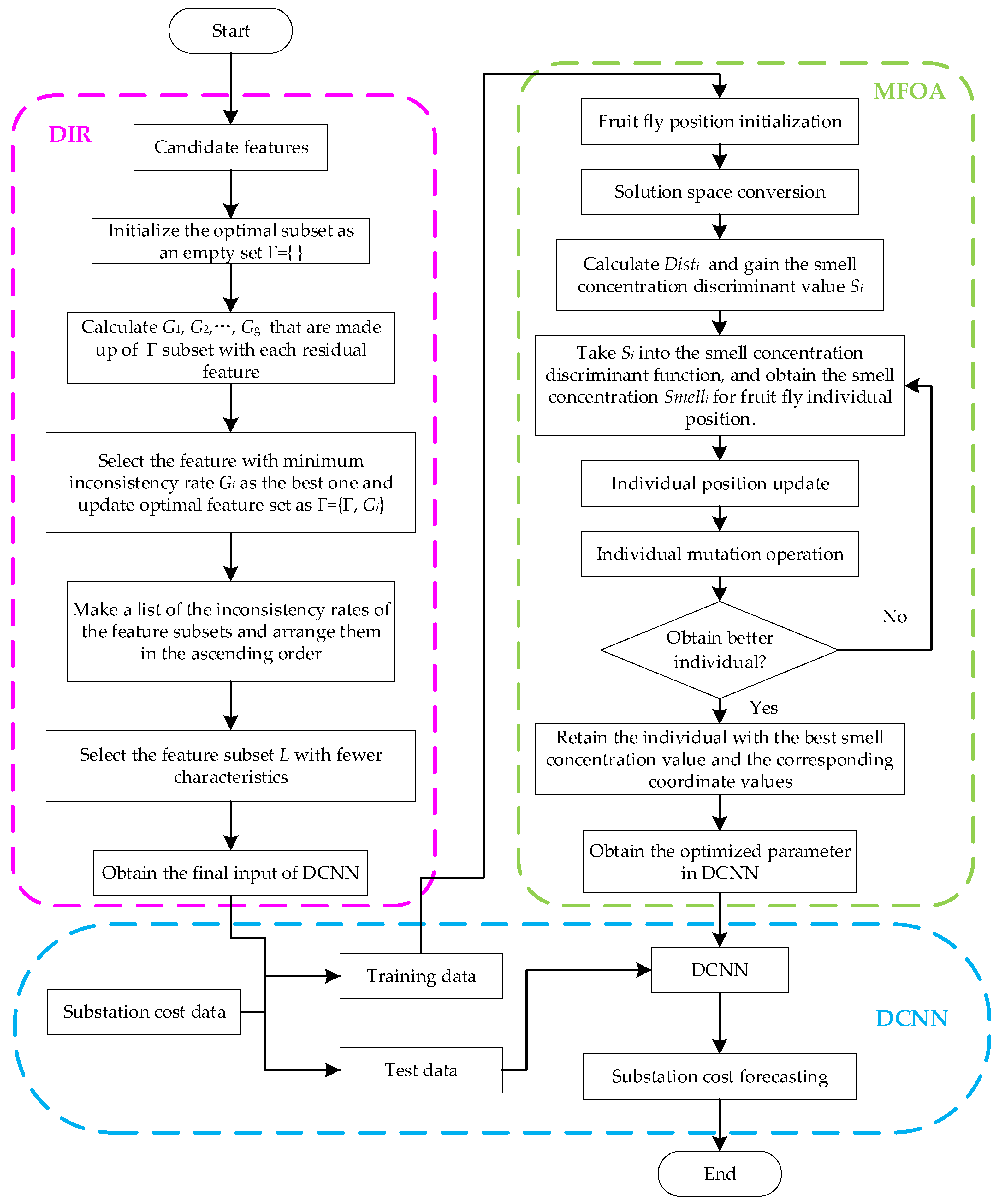
2.4. Approach of MFOA–DIR–DCNN

The framework of the established technique MFOA–DIR–DCNN for substation project cost prediction is displayed in Figure 3. The specific procedures of this novel method can be explained at length as follows:

Figure 3. The flow chart of the modified fruit fly optimization algorithm– data inconsistency rate– deep convolutional neural network (MFOA–DIR–DCNN).

(1)

Determine the initial candidate features of substation project cost. In the DIR, initialize the optimal subset as an empty set $\mathsf{\Gamma }=\left\{\right\}$.

(2)

Complete parameter initialization in the MFOA. By trying a combination of multiple parameter settings, the best parameter initialization supposes that the maximum iteration number equals 200; the scope of the fruit fly position and random flight distance are set as [0, 10] and [−1, 1], respectively.

(3)

Calculate inconsistency. Compute the inconsistency of $G_1,G_2,\dots ,G_g$ that is made up of $\mathsf{\Gamma }$ subsets with each residual feature. The feature with minimum inconsistency rate $G_i$ is selected as the best one, and the updated optimal feature is set as $\mathsf{\Gamma }=\left\{\mathsf{\Gamma },G_i\right\}$.

(4)

Derive the optimal feature subset along with the best values of parameters in the DCNN. The feature subset at current iteration is brought into the DCNN, and both prediction accuracy $r\left(j\right)$ and fitness value $Fitness\left(j\right)$ can be calculated for this training process. Then, determine whether each iteration satisfies the termination requirements (reach the target error value or the maximum number of iterations). If not, reinitialize the feature subset and repeat the above steps until the conditions are met. It is noteworthy that the parameters in the DCNN also need to be optimized, and the initial values of weight $w$ and threshold $\theta$ are randomly assigned. Therefore, a fitness function based on both forecasting precision and feature selection quantity is set up, as shown in Equation (36):

$$Fitness(j)=-(a+r(j)+\frac{b}{Numfeature(j)})$$

(36)

where $Numfeature\left(j\right)$ represents the quantity of selected best characteristics in each iteration, and $a$ and $b$ equal the constants in [0, 1].

(5)

Forecast via the DCNN. When the iterative number reaches the maximum, the estimation stops. Here, the optimal feature subset, the best values of $w$, and $\theta$ are taken into the DCNN model for substation project cost forecasting.

3. Case Study

3.1. Data Processing

This paper selected the cost data of 128 substation projects in various voltage levels and in different areas from 2015 to 2018, as shown in Table 1; the statistics of the substation features are shown in Table A1. In this paper, we selected the cost and corresponding influential factors of the first 66 projects as a training set. Correspondingly, the remaining data were employed as a testing set.

Table 1. Original cost data of projects (Unit: CNY/kV·A).

Serial Number	Cost	Serial Number	Cost	Serial Number	Cost	Serial Number	Cost
1	358.3	33	980.6	65	336.8	97	317.1
2	324.2	34	286.8	66	339.5	98	308.0
3	368.9	35	279.5	67	342.1	99	298.9
4	370.2	36	308.6	68	344.7	100	289.9
5	450.1	37	312.8	69	244.2	101	280.8
6	266.5	38	315.9	70	346.8	102	271.7
7	301.6	39	364.2	71	349.5	103	262.6
8	325.8	40	361.3	72	352.1	104	253.5
9	310.3	41	375.6	73	394.7	105	244.5
10	405.6	42	389.9	74	405.6	106	235.4
11	392.5	43	372.5	75	428.2	107	326.3
12	448.2	44	383.9	76	443.0	108	217.2
13	305.8	45	295.6	77	459.8	109	208.1
14	356.9	46	270.2	78	493.3	110	199.1
15	1058.6	47	260.8	79	289.4	111	390.0
16	501.2	48	240.7	80	293.7	112	280.9
17	337.1	49	223.3	81	297.9	113	285.1
18	304.5	50	239.3	82	402.2	114	476.5
19	291.8	51	381.7	83	491.5	115	449.3
20	279.2	52	406.9	84	491.3	116	470.4
21	299.3	53	315.6	85	212.6	117	491.8
22	285.6	54	285.5	86	452.6	118	306.4
23	305.5	55	252.5	87	353.7	119	310.7
24	208.6	56	214.5	88	254.8	120	274.9
25	356.2	57	325.8	89	155.9	121	319.2
26	401.5	58	328.4	90	375.9	122	283.4
27	378.6	59	311.1	91	375.9	123	369.5
28	369.5	60	333.7	92	397.0	124	373.8
29	253.8	61	336.3	93	418.1	125	398.6
30	300.5	62	309.0	94	344.3	126	244.8
31	272.7	63	341.6	95	335.3	127	256.9
32	423.4	64	334.2	96	326.2	128	472.9

Here, the construction types of substation projects can be divided into three categories: New substation, extended main transformer, and extended interval engineering are valued at 1, 2 and 3, respectively. The substation types were decomposed into three types where the indoor, the semi-indoor, and the outdoor were set as 1, 2 and 3, respectively. The landforms were parted into eight kinds, namely hillock, hillside field, flat, plain, paddy field, rainfed cropland, mountainous region and depression—these were valued at $\left\{1,2,3,4,5,6,7,8\right\}$. In addition, the local GDP was employed to represent the economic development level of the construction area. The proportion of bachelor degree or above in the staff stood for the technical level of the designers. The difference between actual progress and the schedule stipulated in the contract was utilized on behalf of construction progress level. The data needed to be normalized with Equation (37).

$$Y=\left\{y_i\right\}=\frac{x_i-x_{\min }}{x_{\max }-x_{\min }}i=1,2,3,\dots ,n$$

(37)

where $x_i$ and $y_i$ represent the actual value and normalized value, respectively, while $x_{\min }$ and $x_{\max }$ equal the minimum and maximum of the sample data, respectively.

3.2. Model Performance Evaluation

Four commonly adopted error criteria are presented in this paper to measure the forecasting precision of substation project cost obtained by all involved approaches.

(1)

Relative error (RE)

$$RE=\frac{x_i-{\widehat{x}}_i}{x_i}\times 100\%$$

(38)

(2)

Root mean square error (RMSE)

$$RMSE=\sqrt{\frac{1}{n}{\displaystyle \sum _{i=1}^n{(\frac{x_i-{\widehat{x}}_i}{x_i})}^2}}$$

(39)

(3)

Mean absolute percentage error (MAPE)

$$MAPE=\frac{1}{n}{\displaystyle \sum _{i=1}^n\left|(x_i-{\widehat{x}}_i)/x_i\right|}\cdot 100\%$$

(40)

(4)

Average absolute error (AAE)

$$AAE=\frac{1}{n}({\displaystyle \sum _{i=1}^n\left|x_i-{\widehat{x}}_i\right|})/(\frac{1}{n}{\displaystyle \sum _{i=1}^n{x}_i})$$

(41)

where $n$ is the number of testing samples, while $x$ and $\widehat{x}$ represent the actual value and predictive value of substation project cost, respectively. The aforementioned indicators are negatively correlated with forecasting precision.

3.3. Feature Selection

The input of the forecasting techniques was determined on the basis of optimal feature subset selection by the DIR. In reference [45], the authors divided the substation project cost into two main types: Primary and secondary production cost and individual project costs associated with site, totaling more than 20 factors. In reference [46], authors selected more than 26 variables including the area and main transformer capacity as the influencing factors of substation cost. Based on the research of the above references, this paper screened 33 variables as the main influencing factors of substation cost, including area, construction type, voltage level of substation, main transformer capacity, transmission line circuits in the low and high voltage sides, topography, schedule, substation type, the number of transformers, the economic development level of the construction area, inflation rate, the price and number of the circuit breaker in the high voltage side, the quantity of low-voltage capacitors, the price of single main transformer, high-voltage fuse, current transformer, power capacitor, reactor, electric buses, arrester, measuring instrument, relay protection device, signal system, automatic device, the expense of site leveling and foundation treatment, the technical level of the designers, the number of accidents, engineering deviation rate, construction progress level, rainy days, and snowy days. The program in this paper was run in MATLAB R2018b under Intel Core i5-6300U, 4 G and a Windows 10 system.

The iterative process of feature extraction is displayed in Figure 4, where the accuracy curve and the fitness curve show the forecasting precision of the DCNN and fitness values in different iterations, respectively, while option number indicates the quantity of best characteristics derived from the DIR model, and feature reduction refers to the number of characteristics eliminated by the MFOA.

Figure 4. Convergence curves for feature selection. Note: (a) represents the fitness value, (b) represents the forecasting accuracy, (c) represents the reduced number of candidate feature, and (d) represents the selected number of optimization feature.

As we can see, the MFOA converged at the 39th iteration, and the homologous optimal fitness value and prediction accuracy equaled −0.91% and 98.9%, respectively, This indicates that the fitting ability of the DCNN can be enhanced, and the forecasting precision is able to reach the highest through learning and training. Furthermore, the quantity of chosen characteristics was inclined to be steady when the MFOA ran to the 51th time. Ultimately, the final selected characteristics embodied construction type, voltage level, main transformer capacity, substation type, the number of transformers, the price of single main transformer, and the area by eliminating 26 redundant features from 33 candidates. The importance of these seven features derived from the DIR was ordered as (from important to unimportant): The price of single main transformer, the number of transformers, main transformer capacity, construction type, area, substation type, and voltage level.

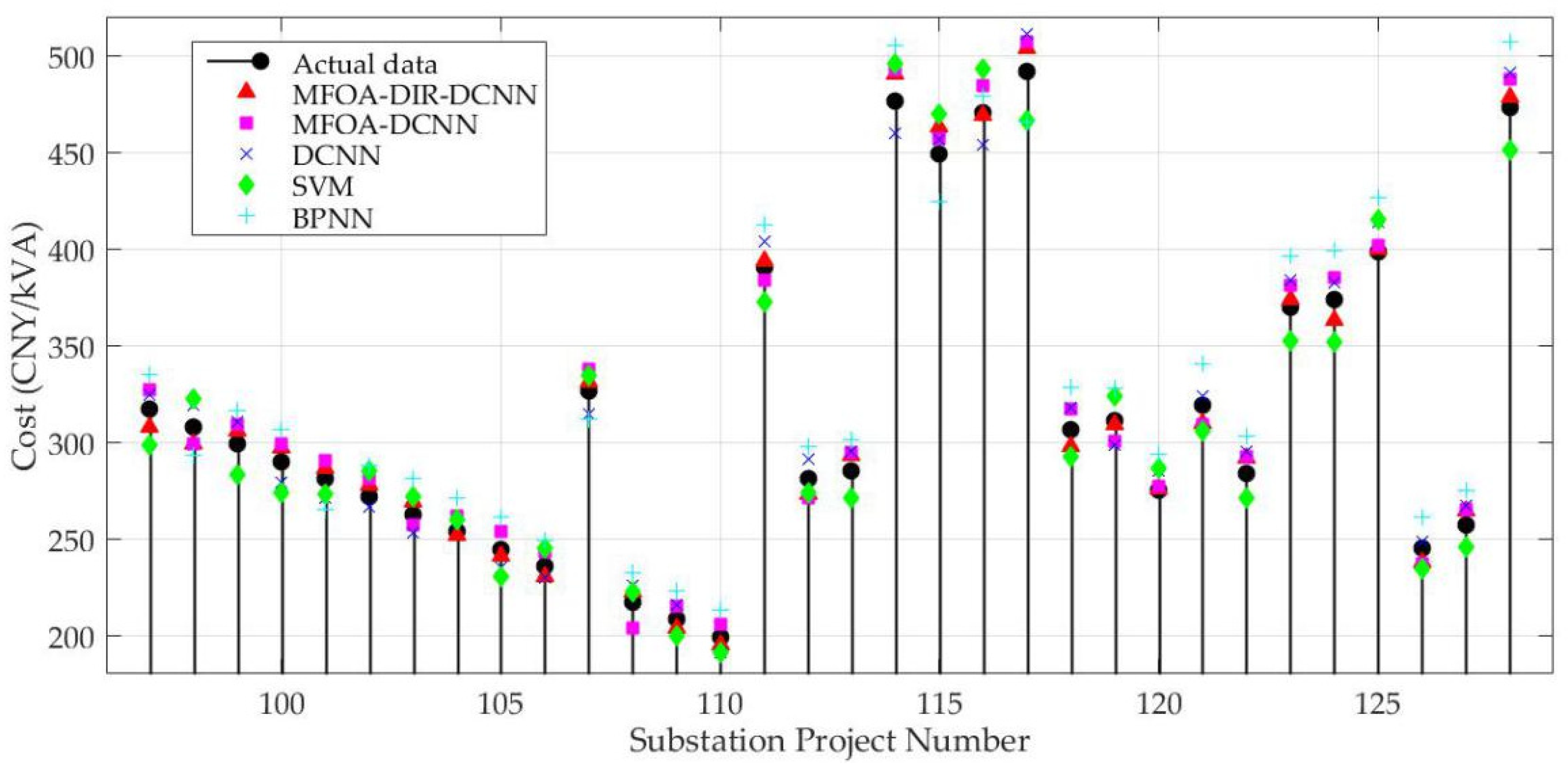
3.4. Results and Discussion

After the accomplishment of feature selection, the input vector was brought into the DCNN model for training and testing. Here, the wavelet kernel function [47], one of the most widely used kernel functions, was applied, and the parameters optimized by MFOA equaled: $\gamma =43.0126$, $\sigma =19.0382$.

For the purpose of verifying the performance of the established approach, four other methods incorporating the MFOA–DCNN, the DCNN, an SVM and the BPNN were used for comparison. In the BPNN, the topology was set as 9-7-1. Tansig and purelin were exploited as the transfer function in the hidden layer and the transfer function in the output layer, respectively. In this paper, we set the maximum number of convergence as 200, while the learning rate and the error equaled 0.1 and 0.0001, respectively. The initial values of weights and thresholds were decided by their own training. In the SVM, the penalty parameter c and kernel parameter σ were valued at 10.276 and 0.0013, respectively, and ε in the loss function equaled 2.4375. In the DCNN, $\gamma =15$, $\sigma =5$. Table 2 lists the prediction results of the substation project cost achieved by five different models.

Table 2. Actual and predicted values of the testing sample (Unit: CNY/kV·A).

Serial Number	Actual Value	BPNN	SVM	DCNN	MFOA–DCNN	MFOA–DIR–DCNN
97	317.1	335.3	298.3	324.3	326.7	308.0
98	308.0	292.9	322.4	318.8	298.7	298.8
99	298.9	316.3	283.1	310.5	308.7	305.9
100	289.9	306.6	273.4	278.8	298.9	297.2
101	280.8	265.2	273.0	270.9	290.1	286.5
102	271.7	288.0	284.7	266.1	281.1	278.0
103	262.6	281.0	271.5	253.2	257.3	269.0
104	253.5	270.9	259.8	257.5	261.9	251.6
105	244.5	261.1	230.3	234.7	253.5	240.9
106	235.4	248.7	244.8	229.6	243.1	230.2
107	326.3	312.0	334.1	314.3	337.9	330.8
108	217.2	232.5	222.4	225.9	203.9	222.5
109	208.1	222.8	199.6	216.0	215.1	203.8
110	199.1	212.8	191.0	191.2	205.4	194.7
111	390.0	412.0	372.3	403.8	383.8	393.9
112	280.9	297.5	273.8	290.7	271.2	273.3
113	285.1	300.8	271.1	295.3	294.6	293.1
114	476.5	504.8	495.9	459.6	492.4	490.0
115	449.3	424.1	469.9	456.0	456.9	462.7
116	470.4	479.0	493.3	453.7	484.6	468.8
117	491.8	465.7	466.3	511.1	507.0	503.6
118	306.4	328.1	292.3	317.4	316.8	298.0
119	310.7	328.0	323.9	298.3	300.6	309.1
120	274.9	294.0	286.4	285.3	277.1	275.6
121	319.2	340.2	305.5	323.8	308.8	309.7
122	283.4	303.3	271.2	294.7	292.6	291.4
123	369.5	396.0	352.3	383.5	381.0	373.7
124	373.8	399.2	351.6	382.3	385.1	363.1
125	398.6	426.2	415.1	413.6	401.8	399.5
126	244.8	260.9	234.3	248.3	236.9	237.5
127	256.9	274.9	245.8	267.2	265.2	264.2
128	472.9	506.9	451.0	490.8	487.6	478.4

For a more intuitive analysis, Figure 5 presents the predictive values and Figure 6 exhibits the values of RE derived from the forecasting techniques. The forecasting error range of the MFOA–DIR–DCNN was within [−3%, 3%], while the number of error points of the MFOA–DCNN and the DCNN in this scope was 5 and 3 (that is, No.102, RE = −2.07%; No.121, RE = 1.44%; No.124, RE = 2.28%), respectively. Among them, the number of error points obtained from the MFOA–DIR–DCNN controlled in [−1%, 1%] equaled 5 (namely No.104, RE = −0.77%; No.116, RE = −0.35%; No.119, RE = −0.50%; No.120, RE = 0.23%; No.125, RE = 0.23%), while the corresponding number of the MFOA–DCNN and the DCNN was 2 (No.120, RE = 0.79%; No.125, RE = −0.82%) and 0, respectively. It can be seen the error points of the SVM mostly ranged in [−6%, −4%] and [4%, 6%], while there existed a large fluctuation in the errors of the BPNN, mainly in [−7%, −5%] and [5%, 7%]. In addition, the minimum absolute values of RE for the MFOA–DIR–DCNN, the MFOA–DCNN, the DCNN, the SVM and the BPNN were 0.23%, 0.79%, 1.44%, −2.52%, 2.83%, respectively, and the maximum absolute values of RE correspondingly equaled 2.99%, 6.12%, 6.51%, −6.94% and 7.17%, respectively. In this respect, these models can be sorted by the forecasting accuracy from the superior to the inferior: the MFOA–DIR–DCNN, the MFOA–DCNN, the DCNN, the SVM and the BPNN. This demonstrates that the application of the MFOA contributes to the enhancement of training and learning process as well as the improvement of global searching ability for the DCNN. Simultaneously, the input derived from the MFOA–DIR can obtain satisfactory prediction results. In contrast with the SVM and the BPNN, this indicates that the DCNN can achieve a better forecasting performance than shallow learning algorithms.

Figure 5. Forecasting results.

Figure 6. Relative error (RE) of prediction methods.

Figure 7 illustrates the comparative results gauged by the RMSE, the MAPE, and the AAE. THis proves that the established hybrid model is superior to the other four techniques from the perspective of the aforementioned error criteria. Concretely, the RMSE, the MAPE and the AAE of the MFOA–DIR–DCNN were 2.2345%, 2.1721% and 2.1700%, respectively. Additionally, the RMSEs of the MFOA–DCNN, the DCNN, the SVM and the BPNN were 3.1818%, 3.7103%, 4.5659%, and 6.2336%, respectively, while the MAPE of the corresponding methods equaled 3.2073%, 3.7148%, 4.4318% and 5.8772%, respectively. Accordingly, the AAE of the MFOA–DCNN, the DCNN, the SVM and the BPNN was equivalent to 3.1251%, 3.7253%, 4.4956% and 5.7347%, respectively. Owing to the fact that the DCNN has advantages over shallow learning algorithms, the MFOA was able to complete parameter optimization of the DCNN, and the DIR approach guarantees the completeness of the input information while reducing the redundant data, which ameliorates the prediction accuracy and robustness.

Figure 7. Root mean square error (RMSE), mean absolute percentage error (MAPE) and average absolute error (AAE) of the prediction techniques.

For further verification that the proposed method is better, the case was predicted by the methods proposed in Reference [8] (BP neural network), [14] (cuckoo search algorithm and support vector machine), and [36] (modified firefly algorithm and support vector machine). The input of these three models was 33—that is 33 candidate features—and the parameter settings were consistent with those mentioned in the text. Table 3 displays the comparative forecasting results.

Table 3. Comparison with the prediction results of the references’ models.

Model	RMSE	MAPE	AAE
Proposed model	2.2345	2.1721	2.1700
Ref. [8]	6.2336	5.8772	5.7347
Ref. [14]	3.3641	3.4502	3.3122
Ref. [36]	3.2794	3.3471	3.2098

According to Table 3, it can be concluded that the forecasting precision of the established approach outperforms that of References [8,14,36]. The main reasons consist of three points. First, the feature selection process can remove the low correlation factors, thereby reducing the input of the model and reducing the training error of the model. Second, optimizing the parameters of the neural network or the support vector machine can provide the training accuracy of the model. For example, the prediction results of References [14] and [36] were superior to the prediction results of the SVM (mentioned in Figure 7). Third, the DCNN model not only reduces the number of neurons and weights, it also uses the pooling operation to make the input features have displacement, scaling and distortion invariance, thus improving the accuracy and robustness of network training, which is better than the SVM and the BPNN.

However, when training and testing the proposed model, it was found that the amount of sample data in the training set had a relatively large impact on the test results. The larger the sample size of the training set, the better the test results. Due to the limited number of new substation projects each year, when applying the proposed model, it is necessary to collect more data on the cost of the previous substation project cost to ensure that the DCNN can be fully trained.

4. Conclusions

This paper developed a novel hybrid approach for cost forecasting based on the DIR, the DCNN and the MFOA. Firstly, the DIR integrated with the MFOA was adopted for input feature selection. Simultaneously, the MFOA was utilized to realize parameter optimization in the DCNN. Thus, the proposed method could be applied to cost forecasting of substation projects on the foundation of the optimized input subset, as well as the best value of γ and σ. The proposed model outperformed the comparative approaches in terms of prediction precision. The case studies demonstrated that: (a) The use of the DIR is conducive to the elimination of unrelated noises and the improvement of prediction performance. (b) Improving the DCNN with the MFOA presents good performance mainly due to the fact that the MFOA enhances the global searching capability of the method. (c) The ideal prediction results were obtained by numerical examples of substation projects in different regions, different voltage levels, and different scales, which shows that the adaptability and stability of the proposed model are also strong. Therefore, this established approach for cost forecasting based on the MFOA–DIR–DCNN, considering its effectiveness and feasibility, provides an alternative for this field in the electric-power industry.

However, the feature selection methods have been researched more and more recently, and it is very important for substation project cost forecasting. Thus, the new feature selection method will be will be a research focus in the future.

References

- Pal, A.; Vullikanti, A.K.S.; Ravi, S.S. A PMU Placement Scheme Considering Realistic Costs and Modern Trends in Relaying. IEEE Trans. Power Syst. 2017, 32, 552–561. [Google Scholar] [CrossRef]
- Heydt, G.T. A Probabilistic Cost/Benefit Analysis of Transmission and Distribution Asset Expansion Projects. IEEE Trans. Power Syst. 2017, 32, 4151–4152. [Google Scholar] [CrossRef]
- Hu, L.X. Research on Prediction of Architectural Engineering Cost based on the Time Series Method. J. Taiyuan Univ. Technol. 2012, 43, 706–709. [Google Scholar]
- Wei, L.; Yuan, Y.-n.; Dong, W.-d.; Zhang, B. Study on engineering cost forecasting of electric power construction based on time response function optimization grey model. In Proceedings of the IEEE, International Conference on Communication Software and Networks, Xi’an, China, 27–29 May 2011; pp. 58–61. [Google Scholar]
- Wei, L. A Model of Building Project Cost Estimation Based on Multiple Structur Integral Linear Regression. Archit. Technol. 2015, 46, 846–849. [Google Scholar]
- Li, J.; Wang, R.; Wang, J.; Li, Y. Analysis and forecasting of the oil consumption in China based on combination models optimized by artificial intelligence algorithms. Energy 2018, 144, 243–264. [Google Scholar] [CrossRef]
- Wang, M.; Zhao, L.; Du, R.; Wang, C.; Chen, L.; Tian, L.; Stanley, H.E. A novel hybrid method of forecasting crude oil prices using complex network science and artificial intelligence algorithms. Appl. Energy 2018, 220, 480–495. [Google Scholar] [CrossRef]
- Ling, Y.P.; Yan, P.F.; Han, C.Z.; Yang, C.G. BP Neural Network Based Cost Prediction Model for Transmission Projects. Electr. Power 2012, 45, 95–99. [Google Scholar]
- Liang, Y.; Niu, D.; Cao, Y.; Hong, W.C. Analysis and Modeling for China’s Electricity Demand Forecasting Using a Hybrid Method Based on Multiple Regression and Extreme Learning Machine: A View from Carbon Emission. Energies 2016, 9, 941. [Google Scholar] [CrossRef]
- Liu, J.; Qing, Y.E. Project Cost Prediction Model Based on BP and RBP Neural Networks in Xiamen City. J. Huaqiao Univ. 2013, 34, 576–580. [Google Scholar]
- Niu, D.; Liang, Y.; Hong, W.C. Wind Speed Forecasting Based on EMD and GRNN Optimized by FOA. Energies 2017, 10, 2001. [Google Scholar] [CrossRef]
- Nieto, P.G.; Lasheras, F.S.; García-Gonzalo, E.; de Cos Juez, F.J. PM 10, concentration forecasting in the metropolitan area of Oviedo (Northern Spain) using models based on SVM, MLP, VARMA and ARIMA: A case study. Sci. Total Environ. 2018, 621, 753–761. [Google Scholar] [CrossRef]
- Peng, G.; Si, H.; Yu, J.; Yang, Y.; Li, S.; Tan, K. Modification and application of SVM algorithm. Comput. Eng. Appl. 2011, 47, 218–221. [Google Scholar]
- Niu, D.; Zhao, W.; Li, S.; Chen, R. Cost Forecasting of Substation Projects Based on Cuckoo Search Algorithm and Support Vector Machines. Sustainability 2018, 10, 118. [Google Scholar] [CrossRef]
- Zhu, X.; Xu, Q.; Tang, M.; Nie, W.; Ma, S.; Xu, Z. Comparison of two optimized machine learning models for predicting displacement of rainfall-induced landslide: A case study in Sichuan Province, China. Eng. Geol. 2017, 218, 213–222. [Google Scholar] [CrossRef]
- Bai, Y.; Chen, Z.; Xie, J.; Li, C. Daily reservoir inflow forecasting using multiscale deep feature learning with hybrid models. J. Hydrol. 2016, 532, 193–206. [Google Scholar] [CrossRef]
- Larson, D.B.; Chen, M.C.; Lungren, M.P.; Halabi, S.S.; Stence, N.V.; Langlotz, C.P. Performance of a Deep-Learning Neural Network Model in Assessing Skeletal Maturity on Pediatric Hand Radiographs. Radiology 2017, 287, 313–322. [Google Scholar] [CrossRef]
- Siddiqui, S.A.; Salman, A.; Malik, M.I.; Shafait, F.; Mian, A.; Shortis, M.R.; Harvey, E.S. Automatic fish species classification in underwater videos: Exploiting pretrained deep neural network models to compensate for limited labelled data. Ices J. Mar. Sci. 2018, 75, 374–389. [Google Scholar] [CrossRef]
- Yu, X.; Dong, H. PTL-CFS based deep convolutional neural network model for remote sensing classification. Computing 2018, 100, 773–785. [Google Scholar] [CrossRef]
- Chen, Y.H.; Krishna, T.; Emer, J.S.; Sze, V. Eyeriss: An Energy-Efficient Reconfigurable Accelerator for Deep Convolutional Neural Networks. IEEE J. Solid State Circuits 2017, 52, 127–138. [Google Scholar] [CrossRef]
- Rawat, W.; Wang, Z. Deep Convolutional Neural Networks for Image Classification: A Comprehensive Review. Neural Comput. 2017, 29, 2352–2449. [Google Scholar] [CrossRef]
- Wang, H.; Yi, H.; Peng, J.; Wang, G.; Liu, Y.; Jiang, H.; Liu, W. Deterministic and probabilistic forecasting of photovoltaic power based on deep convolutional neural network. Energy Convers. Manag. 2017, 153, 409–422. [Google Scholar] [CrossRef]
- Wang, H.Z.; Li, G.Q.; Wang, G.B.; Peng, J.C.; Jiang, H.; Liu, Y.T. Deep learning based ensemble approach for probabilistic wind power forecasting. Appl. Energy 2017, 188, 56–70. [Google Scholar] [CrossRef]
- Liu, H.; Mi, X.; Li, Y. Smart deep learning based wind speed prediction model using wavelet packet decomposition, convolutional neural network and convolutional long short term memory network. Energy Convers. Manag. 2018, 166, 120–131. [Google Scholar] [CrossRef]
- Gunduz, H.; Yaslan, Y.; Cataltepe, Z. Intraday prediction of Borsa Istanbul using convolutional neural networks and feature correlations. Knowl. Based Syst. 2017, 137, 138–148. [Google Scholar] [CrossRef]
- Jin, K.H.; McCann, M.T.; Froustey, E.; Unser, M. Deep Convolutional Neural Network for Inverse Problems in Imaging. IEEE Trans. Image Process. 2017, 26, 4509–4522. [Google Scholar] [CrossRef]
- Pan, W.T. A new Fruit Fly Optimization Algorithm: Taking the financial distress model as an example. Knowl. Based Syst. 2012, 26, 69–74. [Google Scholar] [CrossRef]
- Yang, Q.; Chen, W.N.; Yu, Z.; Gu, T.; Li, Y.; Zhang, H.; Zhang, J. Adaptive Multimodal Continuous Ant Colony Optimization. IEEE Trans. Evol. Comput. 2017, 21, 191–205. [Google Scholar] [CrossRef]
- Chen, Z.; Xiong, R.; Cao, J. Particle swarm optimization-based optimal power management of plug-in hybrid electric vehicles considering uncertain driving conditions. Energy 2016, 96, 197–208. [Google Scholar] [CrossRef]
- Lin, J.; Sheng, G.; Yan, Y.; Dai, J.; Jiang, X. Prediction of Dissolved Gas Concentrations in Transformer Oil Based on the KPCA-FFOA-GRNN Model. Energies 2018, 11, 225. [Google Scholar] [CrossRef]
- Niu, D.; Ma, T.; Liu, B. Power load forecasting by wavelet least squares support vector machine with improved fruit fly optimization algorithm. J. Comb. Optim. 2016, 33, 1122–1143. [Google Scholar]
- Hu, R.; Wen, S.; Zeng, Z.; Huang, T. A short-term power load forecasting model based on the generalized regression neural network with decreasing step fruit fly optimization algorithm. Neurocomputing 2017, 221, 24–31. [Google Scholar] [CrossRef]
- Cao, G.; Wu, L. Support vector regression with fruit fly optimization algorithm for seasonal electricity consumption forecasting. Energy 2016, 115, 734–745. [Google Scholar] [CrossRef]
- Qu, Z.; Zhang, K.; Wang, J.; Zhang, W.; Leng, W. A Hybrid Model Based on Ensemble Empirical Mode Decomposition and Fruit Fly Optimization Algorithm for Wind Speed Forecasting. Adv. Meteorol. 2016, 2016, 3768242. [Google Scholar] [CrossRef]
- Li, H.Z.; Guo, S.; Li, C.J.; Sun, J.Q. A hybrid annual power load forecasting model based on generalized regression neural network with fruit fly optimization algorithm. Knowl. Based Syst. 2013, 37, 378–387. [Google Scholar] [CrossRef]
- Song, Z.; Niu, D.; Xiao, X.; Zhu, L. Substation Engineering Cost Forecasting Method Based on Modified Firefly Algorithm and Support Vector Machine. Electr. Power 2017, 50, 168–178. [Google Scholar]
- Zhang, C.; Kumar, A.; Ré, C. Materialization Optimizations for Feature Selection Workloads. ACM Trans. Database Syst. 2016, 41, 2. [Google Scholar] [CrossRef]
- Niu, D.; Wang, H.; Chen, H.; Liang, Y. The General Regression Neural Network Based on the Fruit Fly Optimization Algorithm and the Data Inconsistency Rate for Transmission Line Icing Prediction. Energies 2017, 10, 2066. [Google Scholar]
- Chen, T.; Ma, J.; Huang, S.H.; Cai, A. Novel and efficient method on feature selection and data classification. J. Comput. Res. Dev. 2012, 49, 735–745. [Google Scholar]
- Liu, J.P.; Li, C.L. The Short-Term Power Load Forecasting Based on Sperm Whale Algorithm and Wavelet Least Square Support Vector Machine with DWT-IR for Feature Selection. Sustainability 2017, 9, 1188. [Google Scholar] [CrossRef]
- Li, C.; Li, S.; Liu, Y. A least squares support vector machine model optimized by moth-flame optimization algorithm for annual power load forecasting. Appl. Intell. 2016, 45, 1166–1178. [Google Scholar] [CrossRef]
- Wu, L.; Cao, G. Seasonal SVR with FOA algorithm for single-step and multi-step ahead forecasting in monthly inbound tourist flow. Knowl. Based Syst. 2016, 110, 157–166. [Google Scholar]
- Iscan, H.; Gunduz, M. A Survey on Fruit Fly Optimization Algorithm. In Proceedings of the International Conference on Signal-Image Technology & Internet-Based Systems. IEEE Computer Society, Bangkok, Thailand, 23–27 November 2015; pp. 520–527. [Google Scholar]
- Zhang, F.; Cai, N.; Wu, J.; Cen, G.; Wang, H.; Chen, X. Image denoising method based on a deep convolution neural network. IET Image Process. 2018, 12, 485–493. [Google Scholar] [CrossRef]
- Lu, Y.; Niu, D.; Qiu, J.; Liu, W. Prediction Technology of Power Transmission and Transformation Project Cost Based on the Decomposition-Integration. Math. Probl. Eng. 2015, 2015, 651878. [Google Scholar] [CrossRef]
- Kang, J.X.; Ai, L.S.; Zhang, X.R.; LIU, S.M.; CAO, Y.; MA, L.; CHENG, Z.H. Analysis of Substation Project Cost Influence Factors. J. Northeast Dianli Univ. 2011, 31, 131–136. (In Chinese) [Google Scholar]
- Zhang, L.; Zhou, W.; Jiao, L. Wavelet support vector machine. IEEE Trans. Syst. Man Cybern. Soc. 2004, 34, 34–39. [Google Scholar] [CrossRef]
© 2019 by the authors. Licensee MDPI, Basel, Switzerland. This article is an open access article distributed under the terms and conditions of the Creative Commons Attribution (CC BY) license (http://creativecommons.org/licenses/by/4.0/).