Article

Advanced MPPT Algorithm for Distributed Photovoltaic Systems

1
Department of Electrical Engineering, POSTECH, Pohang 37673, Korea
2
Department of Electronics and Electrical Engineering, Daegu University, Gyeongsan 38453, Korea
*
Author to whom correspondence should be addressed.
Energies 2019, 12(18), 3576; https://doi.org/10.3390/en12183576
Submission received: 22 August 2019 / Revised: 16 September 2019 / Accepted: 18 September 2019 / Published: 19 September 2019

Abstract

:
The basic and adaptive maximum power point tracking algorithms have been studied for distributed photovoltaic systems to maximize the energy production of a photovoltaic (PV) module. However, the basic maximum power point tracking algorithms using a fixed step size, such as perturb and observe and incremental conductance, suffer from a trade-off between tracking accuracy and tracking speed. Although the adaptive maximum power point tracking algorithms using a variable step size improve the maximum power point tracking efficiency and dynamic response of the basic algorithms, these algorithms still have the oscillations at the maximum power point, because the variable step size is sensitive to external factors. Therefore, this paper proposes an enhanced maximum power point tracking algorithm that can have fast dynamic response, low oscillations, and high maximum power point tracking efficiency. To achieve these advantages, the proposed maximum power point tracking algorithm uses two methods that can apply the optimal step size to each operating range. In the operating range near the maximum power point, a small fixed step size is used to minimize the oscillations at the maximum power point. In contrast, in the operating range far from the maximum power point, a variable step size proportional to the slope of the power-voltage curve of PV module is used to achieve fast tracking speed under dynamic weather conditions. As a result, the proposed algorithm can achieve higher maximum power point tracking efficiency, faster dynamic response, and lower oscillations than the basic and adaptive algorithms. The theoretical analysis and performance of the proposed algorithm were verified by experimental results. In addition, the comparative experimental results of the proposed algorithm with the other maximum power point tracking algorithms show the superiority of the proposed algorithm.

1. Introduction

The renewable energy resources including wind power, biomass, solar heating, solar photovoltaic (PV), hydroelectric energy, and fuel cells have been widely used to reduce global warming effects caused by greenhouse gas emission [1,2,3,4]. Among these energy resources, solar PV has attracted attention as a promising renewable energy source due to the following reasons:
  • Diverse applications: PV system can be easily applied to microgrid, households, and buildings [5,6,7].
  • Low maintenance costs: Only PV module, inverter, and cable are required for maintenance and the maintenance period is long [8,9,10].
  • Technology development: Various methods were constantly introduced to improve the technology in the solar power industry [8,9,10].
PV systems consist of PV modules for converting sunlight into direct current (DC) electricity, as well as PV inverters for converting DC into alternating current (AC). Based on the connection method between the PV module and the PV inverter, the PV inverter can be categorized as a central inverter or as a module-level power electronic (MLPE). In the past, central inverters (Figure 1a) connected with series-connected PV modules were widely used because they have the advantages of simple structure and low cost [11]. However, central inverters suffered from significant performance degradation under partial shading due to multiple maximum power points and mismatches in PV modules. To solve the partial shading problem, MLPEs (Figure 1b), which include a DC-optimizer and a micro-inverter, were introduced [12,13,14,15,16]. MLPEs are connected to one PV module and harvest optimum power by performing module-level maximum power point tracking (MPPT); this is also known as distributed MPPT (DMPPT) [17,18,19]. Thereby, MLPEs solve the partial shading problem and improve the performance of an entire PV system.
Among many MPPT algorithms, hill-climbing, perturb and observe (P&O), and incremental conductance (INC) have been widely used due to their simplicity and ease of implementation [20,21,22,23,24].
Hill-climbing and P&O algorithms operate on the same fundamental principle that the variation (ΔVPV) of PV voltage (VPV) and the variation (ΔPPV) of PV power (PPV) become zero at the maximum power point (MPP). The difference between the P&O and hill-climbing algorithms is that P&O uses a PI controller. Operations in both hill-climbing and P&O algorithms can be classified into five modes and are described in Figure 2 and Table 1 [20,21,22,23]. The INC algorithm tracks the MPP based on the principle that the variation (ΔIPV) of PV current (IPV) becomes zero and the slope of −ΔIPVVPV is the same as IPV/VPV at the MPP. The INC algorithm also has five operating modes, and its principle of operation is described in Figure 3 and Table 2 [24]. However, these basic MPPT algorithms have a trade-off problem between tracking accuracy and speed because fixed step size is used for perturbation. If small fixed step size is used, tracking accuracy increases, but speed is slower. In this case, the basic MPPT algorithms can fail to track the MPP under dynamic weather conditions. At large fixed step size, tracking speed is faster, but tracking accuracy decreases, which causes a low MPPT efficiency.
To solve these problems, adaptive hill-climbing, adaptive P&O, and adaptive INC algorithms using variable step sizes were introduced [25,26,27,28]. In each adaptive MPPT algorithm, a variable step size is automatically adjusted according to the slope formula consisting of the variations (ΔPPV and ΔVPV) and variable step coefficients (a, N, and M); a∙ΔPPVVPV in [25,26], N∙ΔPPVVPV in [27], and M∙ΔPPVVPV in [28]. The variable step size becomes high far from the MPP and low near the MPP. Therefore, the adaptive MPPT algorithms can achieve fast tracking speed in the operating range far from the MPP and small oscillations in the operating range near the MPP. However, these algorithms still have oscillations at the MPP because the variables (ΔPPV and ΔVPV) in the slope formula are easily affected by sensing and calculation errors, sensing noise, and ripples of VPV and IPV.
In [29,30,31,32], the MPPT algorithms with intelligent prediction were introduced. Some of the algorithms used fuzzy logic to vary the step size [29,30,31]; the fuzzy logic method consists of fuzzification, a fuzzy rule-based lookup table (Table 3), and defuzzification. First, the input variables (ΔIPV and ΔPPV) are converted into fuzzy subsets such as negative big (NB), negative small (NS), zero (ZO), positive small (PS), and positive big (PB) depending on ΔIPV and ΔPPV. Then, one fuzzy subset is determined based on the rule-based lookup table and it provides a numeric step size. The MPPT algorithm using fuzzy logic is effective in dealing with the nonlinear characteristics of the PV module because the fuzzy logic divides the nonlinear system in the fuzzy subsets defined by the variables (ΔIPV and ΔPPV) and controls the nonlinearity of system using the rule base for each area (See Table 3). Therefore, it can track the MPP well under dynamic weather conditions. However, compared to other MPPT algorithms such as adaptive P&O and INC algorithms, it requires a digital signal processor (DSP) with higher specification and also makes the user’s design more difficult because of its higher complexity of algorithm and execution process [27,31]. This is a disadvantage for commercialization. The other MPPT algorithm of [32] changed the step size by using a PID controller tuned by genetic algorithm. First, the genetic algorithm evaluates a number of solutions known as chromosomes using a fitness function, and later, genetic operators (selection, crossover, and mutation) are applied until a stop criterion is satisfied (Figure 4). Based on this principle of the genetic algorithm, the PID coefficients (Kp, Ki, and Kd) are determined to vary the step size. This MPPT algorithm also has good performance under dynamic weather conditions, but it requires high computational capability and sophisticated controllers due to its complexity.
In this paper, an advanced MPPT algorithm for DMPPT in the MLPEs is proposed, which improves the tracking speed and accuracy under both steady and dynamic weather conditions. Similar to the adaptive MPPT algorithms, the proposed MPPT algorithm automatically changes the variable step size according to the slope of ΔPPVVPV in the operating range far from the MPP. However, in the operating range near the MPP, it accurately tracks the MPP using a small fixed step size. As a result, the proposed MPPT algorithm achieves small oscillations at the MPP and a fast dynamic response. In addition, compared with the MPPT algorithms with intelligent control such as fuzzy logic and PID, the proposed MPPT algorithm can reduce the computational load of DSP because it is based on simple P&O method. Therefore, it allows manufacturers to use cheap DSPs for the PV system.
The distributed PV system and proposed MPPT algorithm are described in Section 2, the experimental results and discussion are presented in Section 3, and a conclusion is given in Section 4.

2. Distributed PV System and Proposed MPPT Algorithm

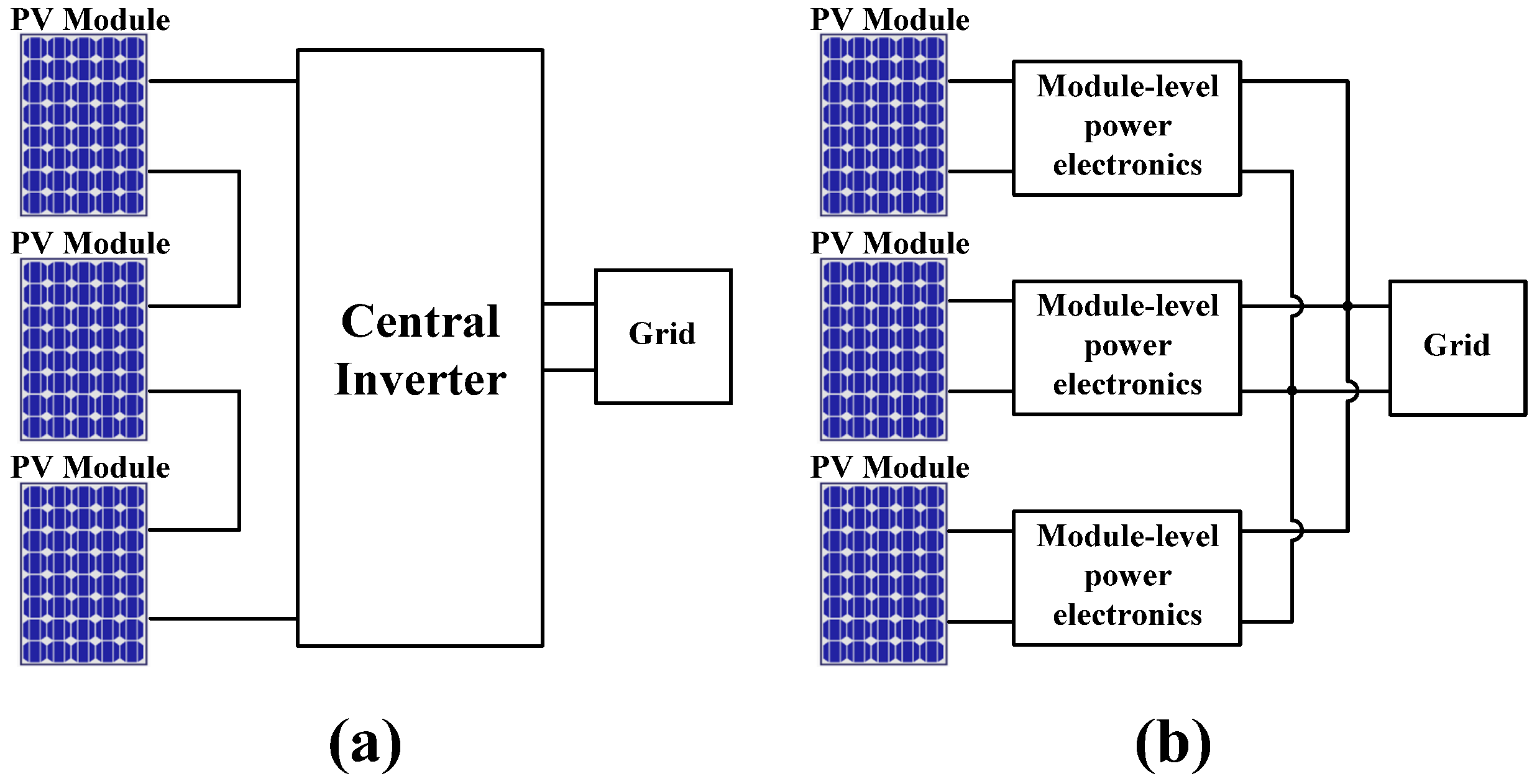
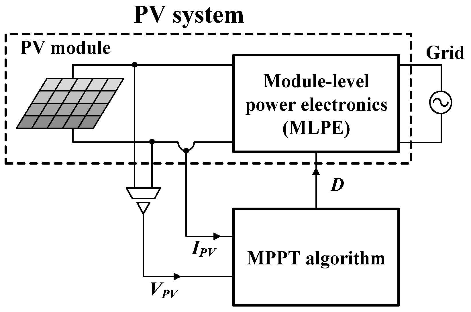
2.1. Distributed PV System
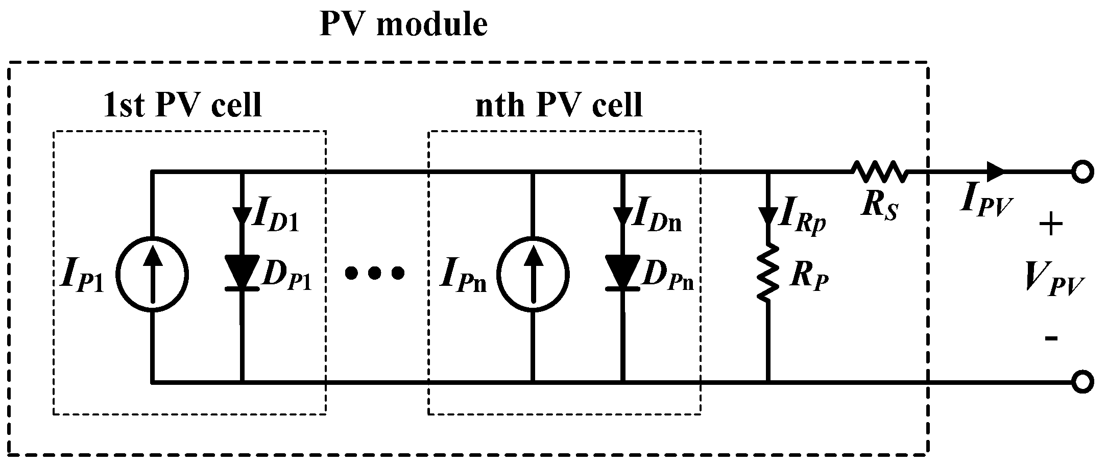
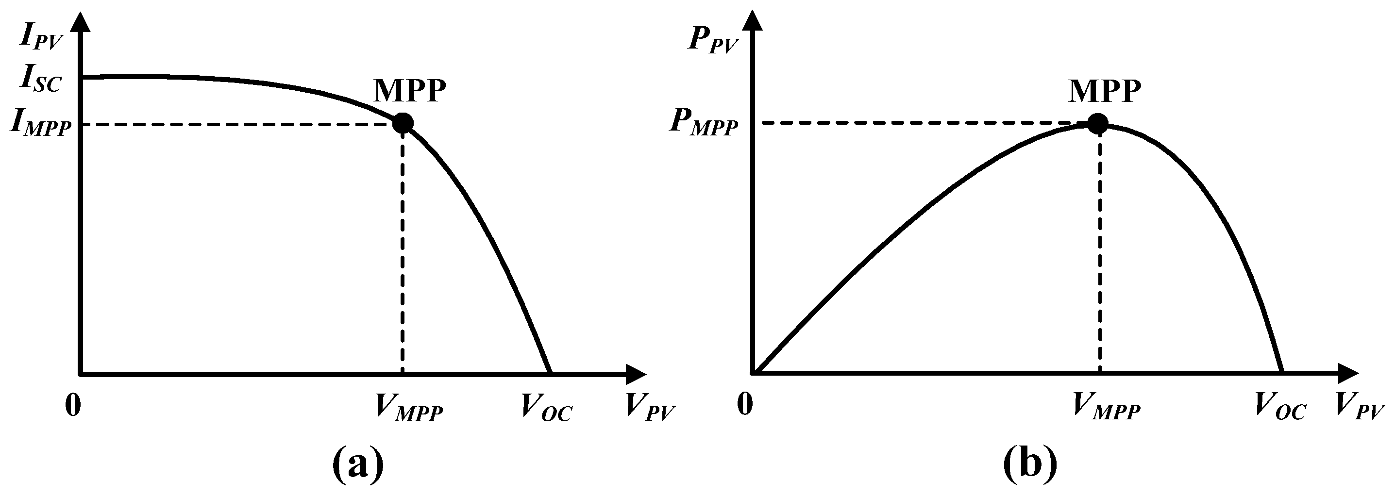
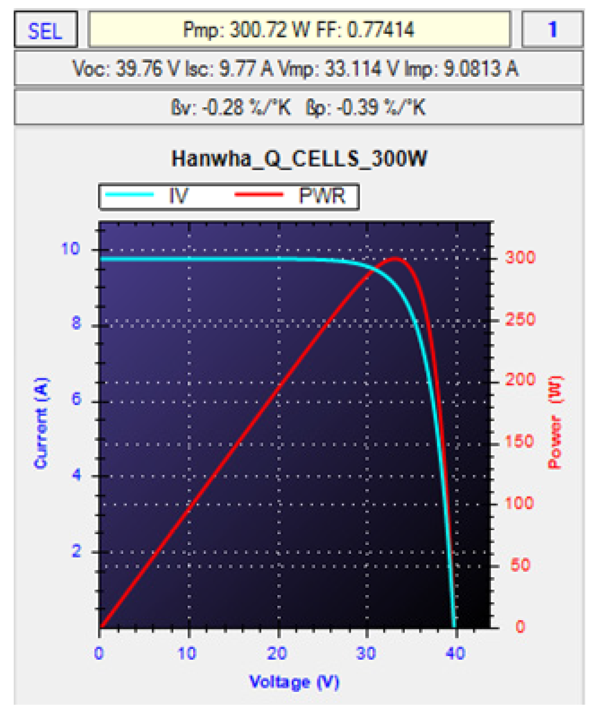
A distributed PV system with the MPPT algorithm is shown in Figure 5; the system consists of one PV module and one MLPE. Due to the fact that the PV module converts sunlight into low DC voltage, the MLPE requires a high voltage gain to convert low DC voltage into high AC voltage with grid frequency. The MPPT algorithm controls the duty ratio (D) of the MLPE to operate at the MPP of the PV module. To perform the MPPT algorithm, the voltage (VPV) and current (IPV) of the PV module are used as input signals.

2.1.1. PV Module

Based on the references [33,34], the equivalent circuit of the PV module can be derived as shown in Figure 6. The PV module consists of several PV cells and two parasitic resistances (RS, RP), where each PV cell has a combined structure of an ideal current source (IP) and a diode (DP). The current (IPV) of the PV module can be derived as
I P V = I P I D I R p
where IP = IP1 + IP2 ⋯ + IPn and ID = ID1 + ID2 ⋯ + IDn. Assuming all PV cells are the same, IP = nIP1 and ID = nID1 are obtained. Using the Shockley diode equation, ID is given by
I D = n I 0 [ e ( V P V + R S I P V ) / ( a n S V t ) 1 ]
where n is the number of PV cells connected in parallel, ns is the number of PV cells connected in series, I0 is the saturation current of the diode, a is the diode ideality constant, and Vt = kT/q is the thermal voltage of the diode with q = 1.602 × 10⁻¹⁹ C, k = 1.381 × 10⁻²³ J/K, and T is an ambient temperature.
As the voltage across RP is given by VPV + RSIPV, the current of RP is obtained as
I R p = V P V + R S I P V R P .
Then, inserting (2) and (3) into (1) results in
I P V = I P n I 0 [ e ( V P V + R S I P V ) / ( a V t ) 1 ] V P V + R S I P V R P .
Using (4), the characteristic curves of the PV module are drawn as shown in Figure 7. Figure 7a shows the current–voltage characteristic curve of the PV module and Figure 7b shows the power–voltage characteristic curve. These curves have notable variables: short-circuit current (ISC), open-circuit voltage (VOC), maximum power point (MPP), voltage at MPP (VMPP), current at MPP (IMPP), and power at MPP (PMPP).
The current of the PV cell depends on the solar irradiance and the temperature as follows;
I P = n [ I P , S T C + K I ( T T n ) ] G G n
where IP,STC is a light-generated current at the standard test condition (STC, 25°C and 1000 W/m2), KI is a temperature coefficient, Tn is a nominal temperature (25°C), G is an irradiation level of the PV module, and Gn is a nominal irradiance level (1000 W/m2). Using (5), Equation (4) can be represented as
I P V = n [ I P , S T C + K I ( T T n ) ] G G n n I 0 [ e ( V P V + R S I P V ) / ( a V t ) 1 ] V P V + R S I P V R P .
Equation (6) shows that the characteristic curve of the PV module can be changed according to the solar irradiance level and the temperature.

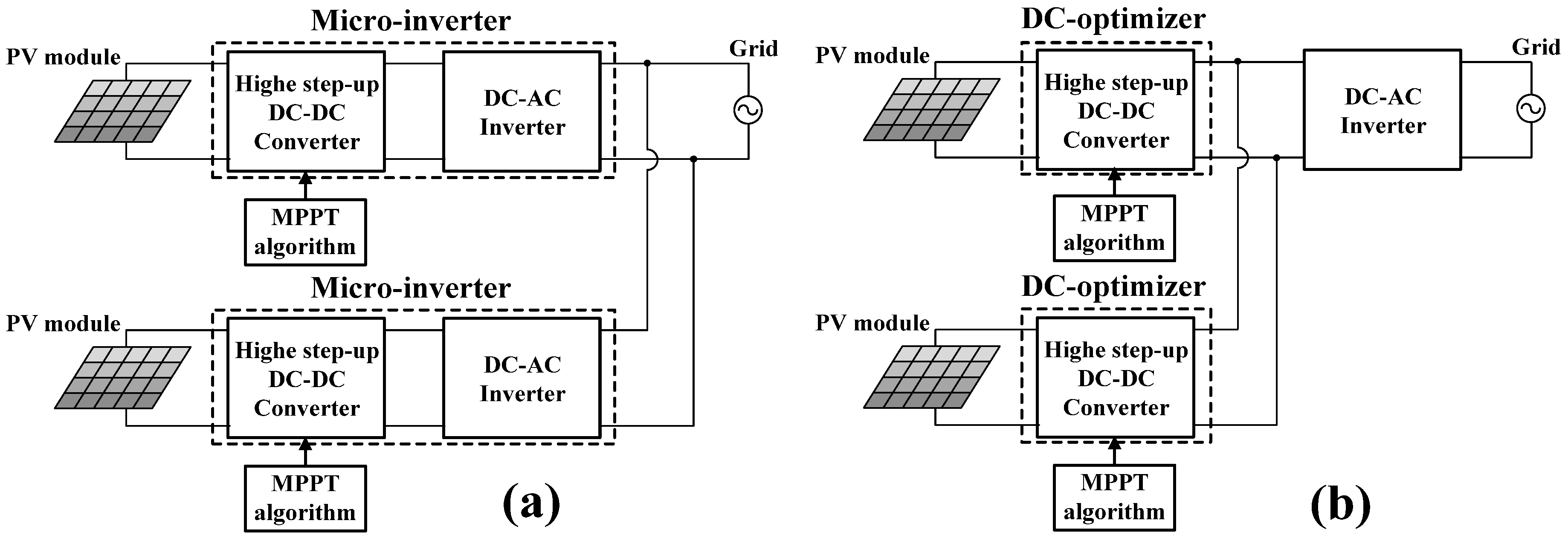
2.1.2. Module-Level Power Electronics (MLPE)

As shown in Figure 8, the MLPE is classified into a micro-inverter and a DC-optimizer. The micro-inverter consists of a DC–DC converter with high voltage gain and a DC–AC inverter, and the DC-optimizer has only one DC–DC converter with high voltage gain. Therefore, the DC-optimizer can cost less than the micro-inverter, but it needs a DC–AC inverter with high power capability. In the micro-inverter and the DC-optimizer, one MPPT algorithm is applied to each DC–DC converter to optimize each PV module. Therefore, the MPPT algorithms used in the MLPEs are called a module-level MPPT, or DMPPT.

2.2. Prospoed MPPT Algorithm

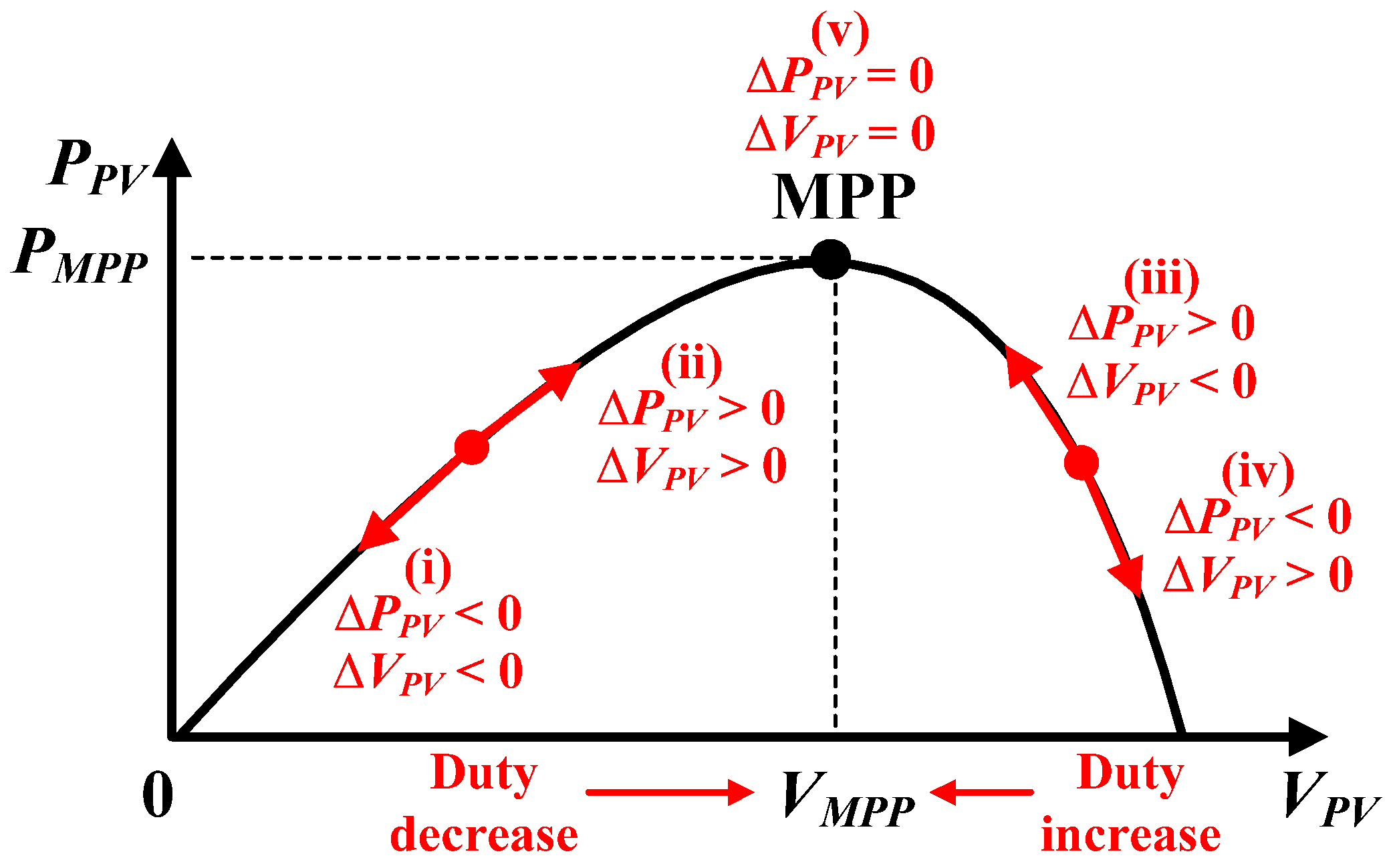
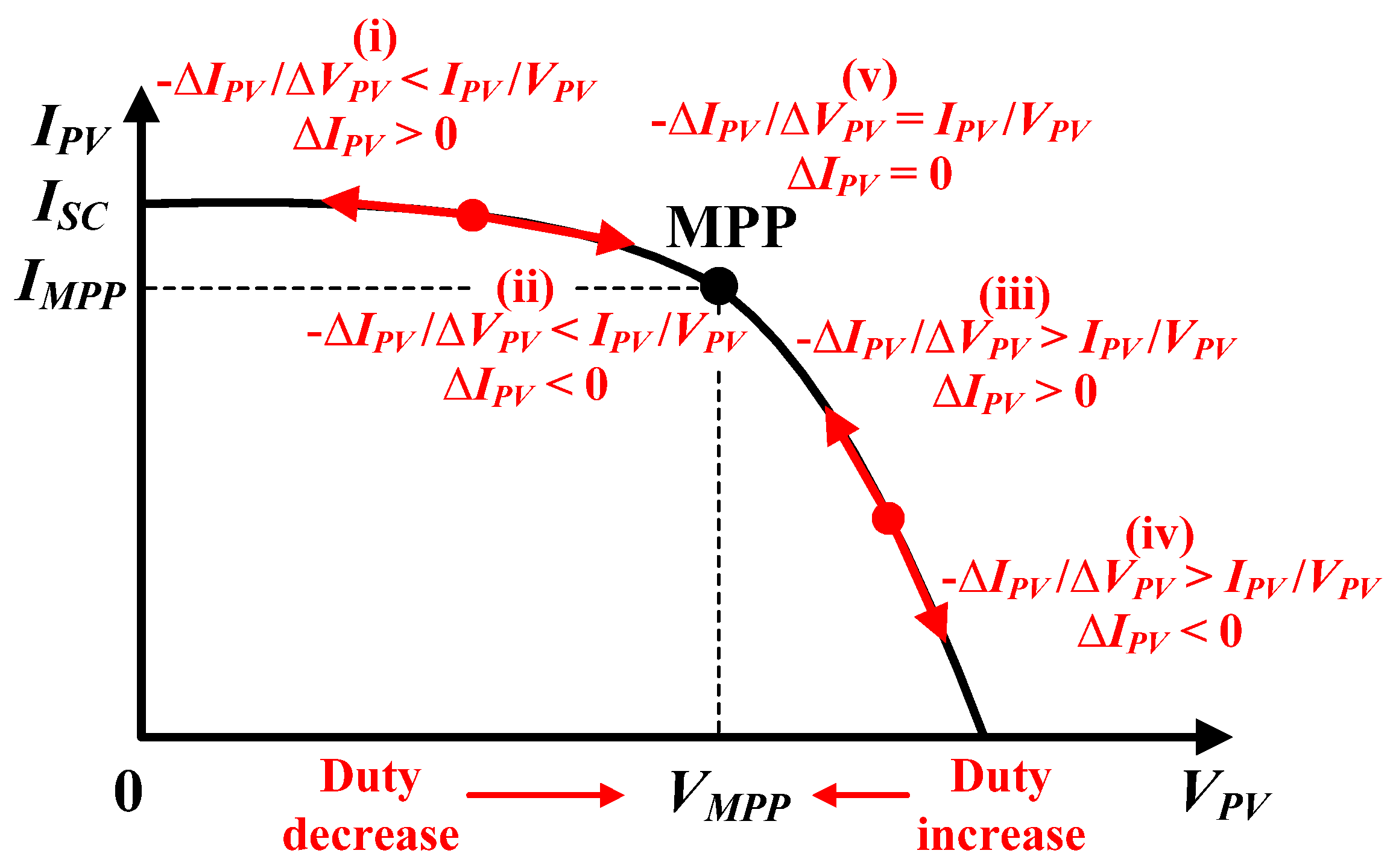
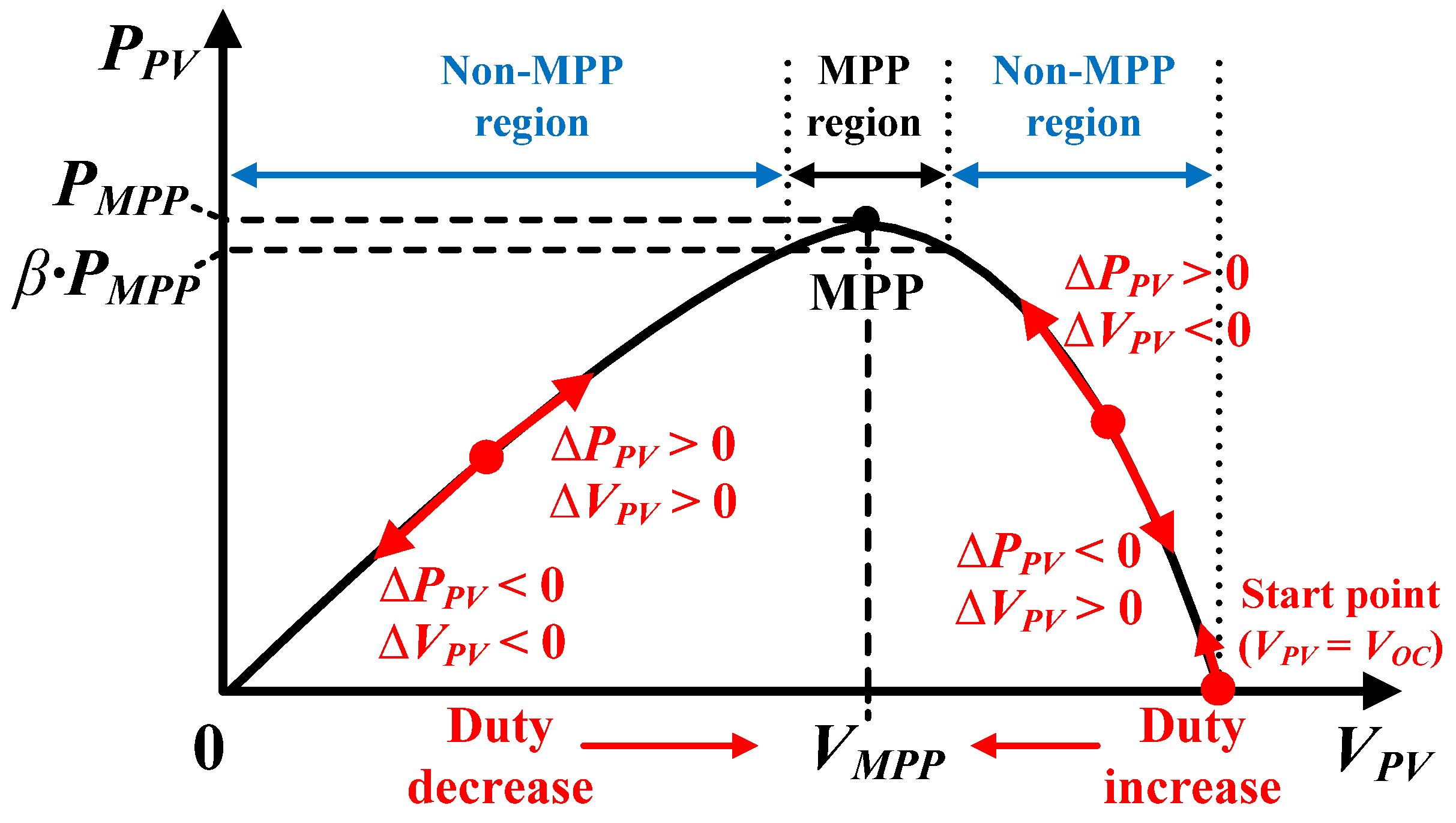
2.2.1. Principle of the Algorithm
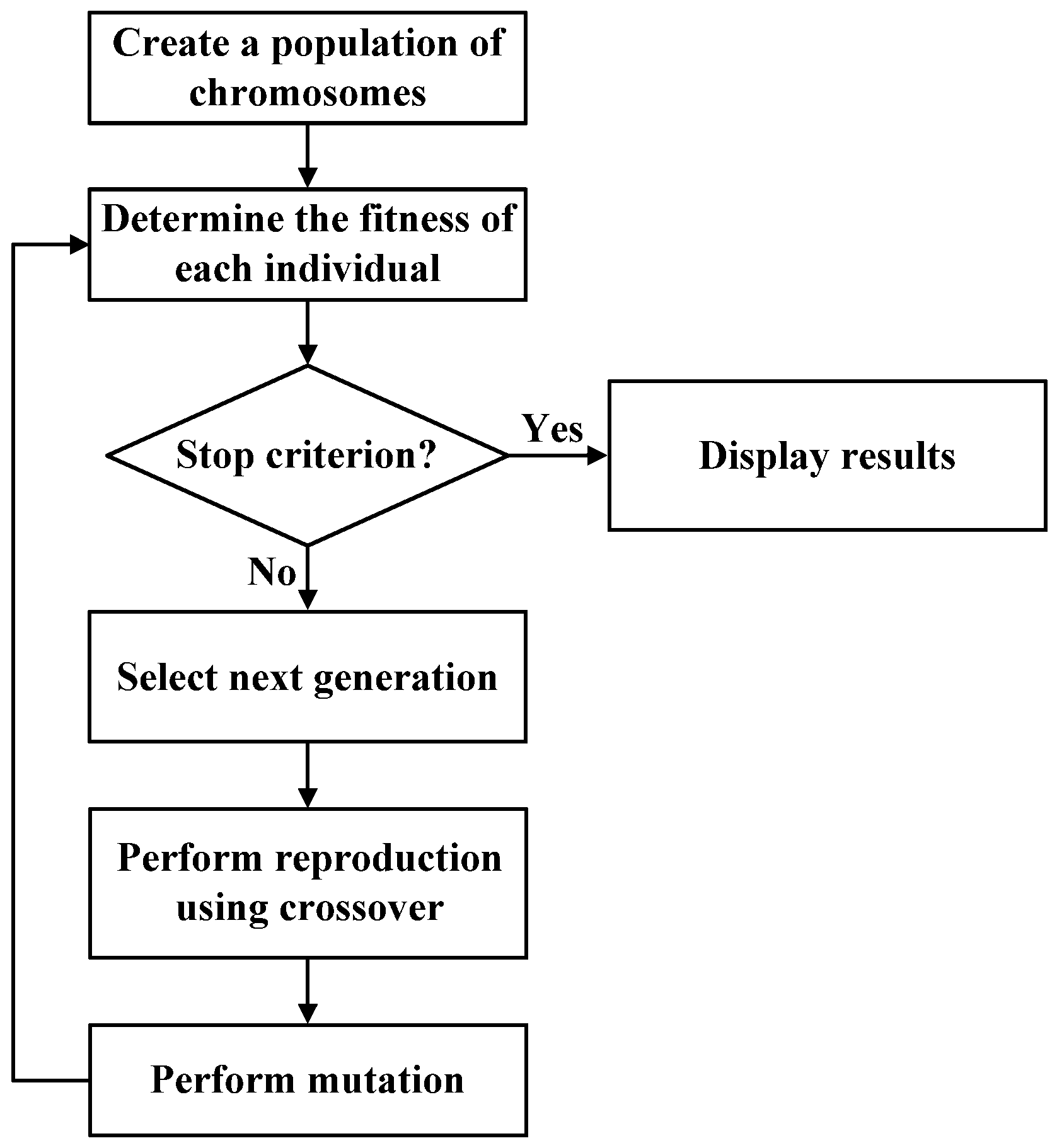
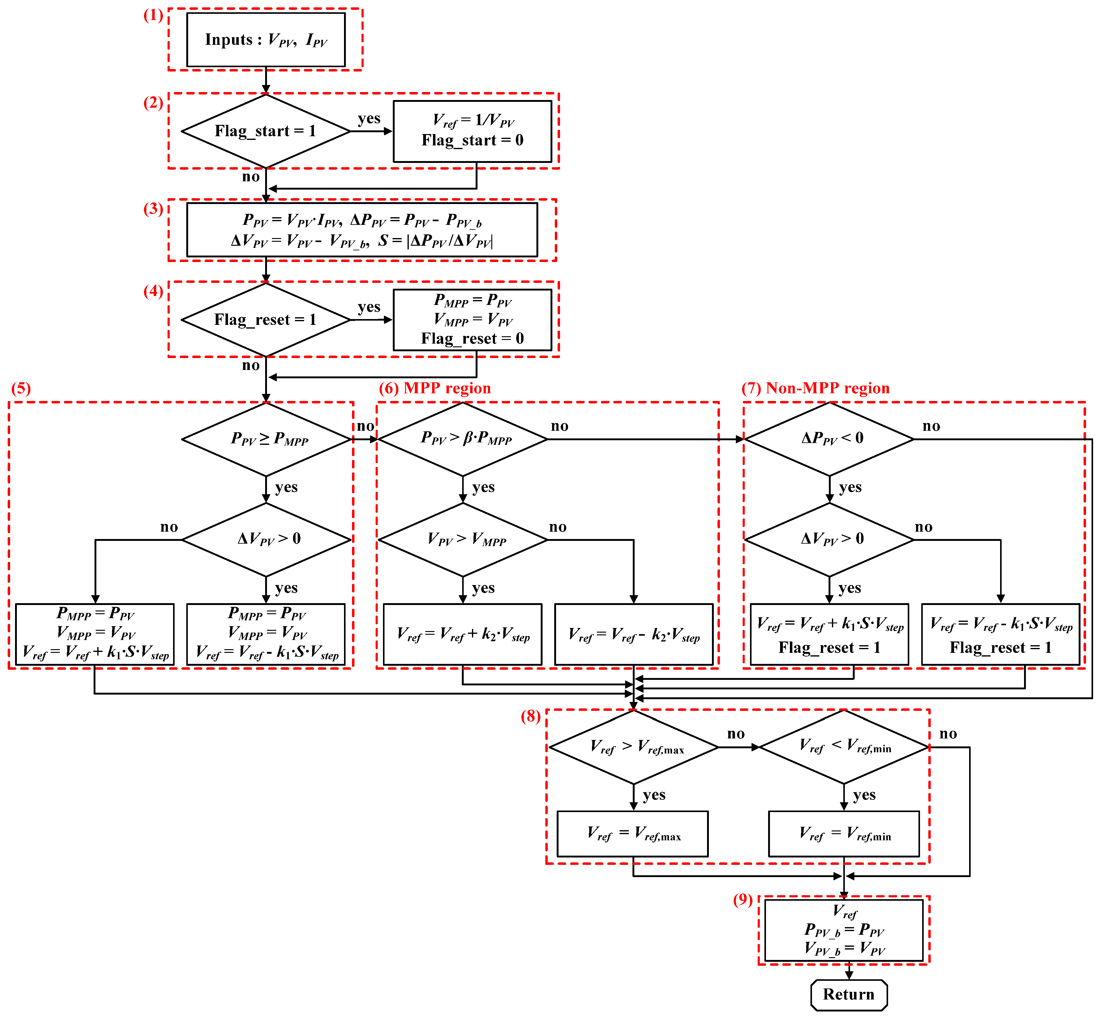
The proposed MPPT algorithm uses two methods that can apply the optimal step size to each operating range. In the operating range far from the MPP (non-MPP region), a variable step size (=k1SVstep) is automatically adjusted according to the slope of ΔPPVVPV for fast dynamic response. Here, k1 is a constant coefficient for variable step size, S is a slope coefficient calculated as |ΔPPVVPV|, and Vstep is a fixed step size. In the operating range near the MPP (MPP region), a small fixed step size (=k2Vstep) is used to minimize the oscillations at the MPP, where k2 is a constant coefficient for small fixed step size.
As shown in Figure 9, the proposed MPPT algorithm has two operating regions including the MPP (PPV > βPMPP) and non-MPP (PPV < βPMPP) regions, where β is an MPP region coefficient. The operating point starts at VPV = VOC and move with fast tracking speed toward the MPP (VMPP, PMPP). The direction of the operating point is determined using ΔPPV and ΔVPV, where Δ means the difference between the present and previous values. In addition, the present PPV is compared with PMPP to search the MPP.

2.2.2. Flow Chart

The flow chart of the proposed MPPT algorithm is shown in Figure 10, and it is described as follows:
  • The present VPV and IPV of the PV module are used as the input signals for the proposed MPPT algorithm. The variable “Flag_start” is preset to 1 for fast tracking speed at the starting point of VPV = VOC, and the variable “Flag_reset” is preset to 1 for setting the PMPP and VMPP to the present PPV and VPV, where PPV = VPVIPV.
  • If Flag_start is 1, it is determined that the operating point is located at the starting point of VPV = VOC. Therefore, the reference variable (Vref) is initially set to 1/VPV (=1/VOC) and the operating point moves rapidly toward the MPP. After that, Flag_start is set to 0.
  • In this process, PPV is calculated as VPVIPV, ΔPPV and ΔVPV are calculated using present (PPV and VPV) and previous (PPV_b and VPV_b) values, and the slope coefficient (S) is calculated as |ΔPPVVPV|.
  • If Flag_reset is 1, PMPP and VMPP are set to the present PPV and VPV, and then Flag_reset is set to 0.
  • If the present PPV is higher than PMPP, it is determined that the MPP has not been found yet. Therefore, the operating point is forced to keep moving toward the MPP, and PMPP and VMPP are reset to the present PPV and VPV. To quickly find the MPP, the variable step size (=k1SVstep) is used in this process.
  • If the operating point is located in the MPP region, the small fixed step size (=k2Vstep) is used to track the MPP accurately.
  • If PPV is lower than the boundary value (βPMPP) between the MPP and non-MPP regions, it is determined that the operating point is located in non-MPP region. This process is usually performed under dynamic weather conditions because the MPP changes under these conditions. Therefore, Flag_reset is set to 1 to find a new MPP, and the variable step size (=k1SVstep) is automatically adjusted according to the slope of ΔPPVVPV for a fast dynamic response.
  • Vref is limited by the maximum and minimum values (Vref,max and Vref,min) of Vref to prevent malfunction of the DC–DC converter in the MLPEs.
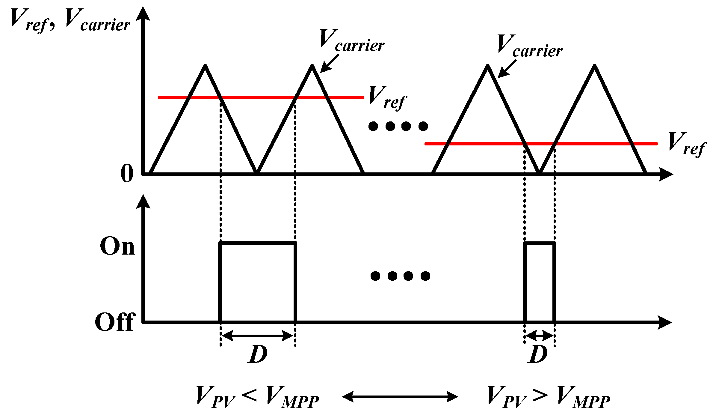
  • Through the above processes, a new Vref is obtained. Vref is compared with the carrier signal (Vcarrier) in the digital signal processor (DSP), and a new duty ratio (D) is generated to control the DC–DC converter in the MLPE (Figure 11). In addition, the previous values (PPV_b and VPV_b) are obtained at this time.
The above processes from (1) to (9) are repeated to operate the DC–DC converter at the MPP of the PV module.

2.2.3. Design Considerations

(1) aximum (Vref,max) and minimum (Vref,min) of Vref
The DC–DC converter in the MLPEs has an input voltage range of VPV,minVPVVPV,max due to its limited voltage gain. Since Vref is calculated as 1/VPV, Vref,max and Vref,min can be defined as 1/VPV,min and 1/VPV,max, respectively.
(2) Coefficient (k1) for variable step size and coefficient (k2) for small fixed step size
The proposed MPPT algorithm uses a variable step size (=k1SVstep) for fast dynamic response in operating range far from the MPP and a small fixed step size (=k2Vstep) for small oscillations in operating range near the MPP, where k1, k2, and Vstep have constant values. Due to the fact that the slope coefficient (S) is calculated as |ΔPPVVPV|, the variation of the reference variable (Vref) is given by
| Δ V r e f | = k 1 | Δ P P V Δ V P V | V s t e p
where Δ means a difference between the present and previous values. The operating point of the proposed MPPT algorithm reaches the MPP (VPV = VMPP, PPV = PMPP) after starting at the point (VPV = VOC, PPV = 0), where VOC is an open-circuit voltage of the PV module. Considering only the starting point and the MPP at the STC (25 °C and 1000 W/m2), the above equation can be represented using Vref = 1/VPV as
1 V M P P , S T C 1 V O C = k 1 P M P P , S T C V O C V M P P , S T C V s t e p
where VMPP,STC and PMPP,STC are the voltage and power at the MPP under the STC (25 °C and 1000 W/m2).
Therefore, k1 can be obtained as
k 1 = ( V O C V M P P , S T C ) 2 V O C V M P P , S T C V s t e p P M P P , S T C .
The small step coefficient (k2) can be determined by considering the resolution of VPV in the operating range near the MPP. If accuracy of the third decimal point of VPV is required in operating range near the MPP, |ΔVref| = k2Vstep can be represented using Vref = 1/VPV as
1 V M P P , S T C 1 V M P P , S T C + 0.001 = k 2 V s t e p .
Therefore, k2 is calculated as
k 2 = 0.001 V M P P , S T C ( V M P P , S T C + 0.001 ) V s t e p .
(3) MPP region coefficient (β)
βPMPP is a boundary value between the MPP and non-MPP regions. For fast dynamic response, β should be close to one; however, if it is too close to one, oscillations can occur at the boundary of PPV = βPMPP. Therefore, β = 0.9~0.95 is recommended.
(4) Fixed step size (Vstep)
To optimize the proposed MPPT algorithm in a given DC–DC converter topology and operating conditions, Vstep is determined after several experiments. Therefore, Vstep has a user-defined value, and Vstep = 10 was used for the experiments in this paper.

3. Experimental Results and Discussion

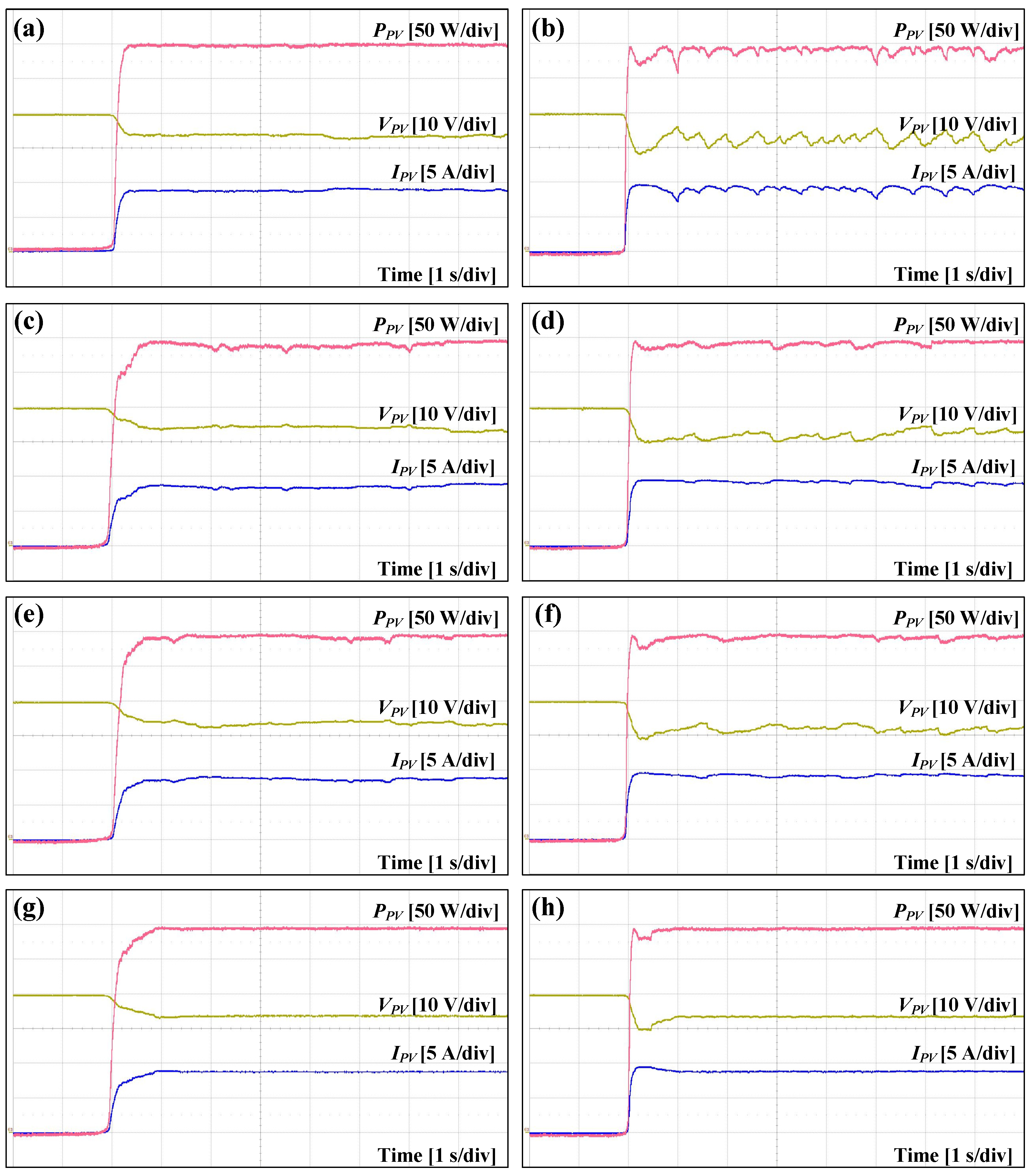
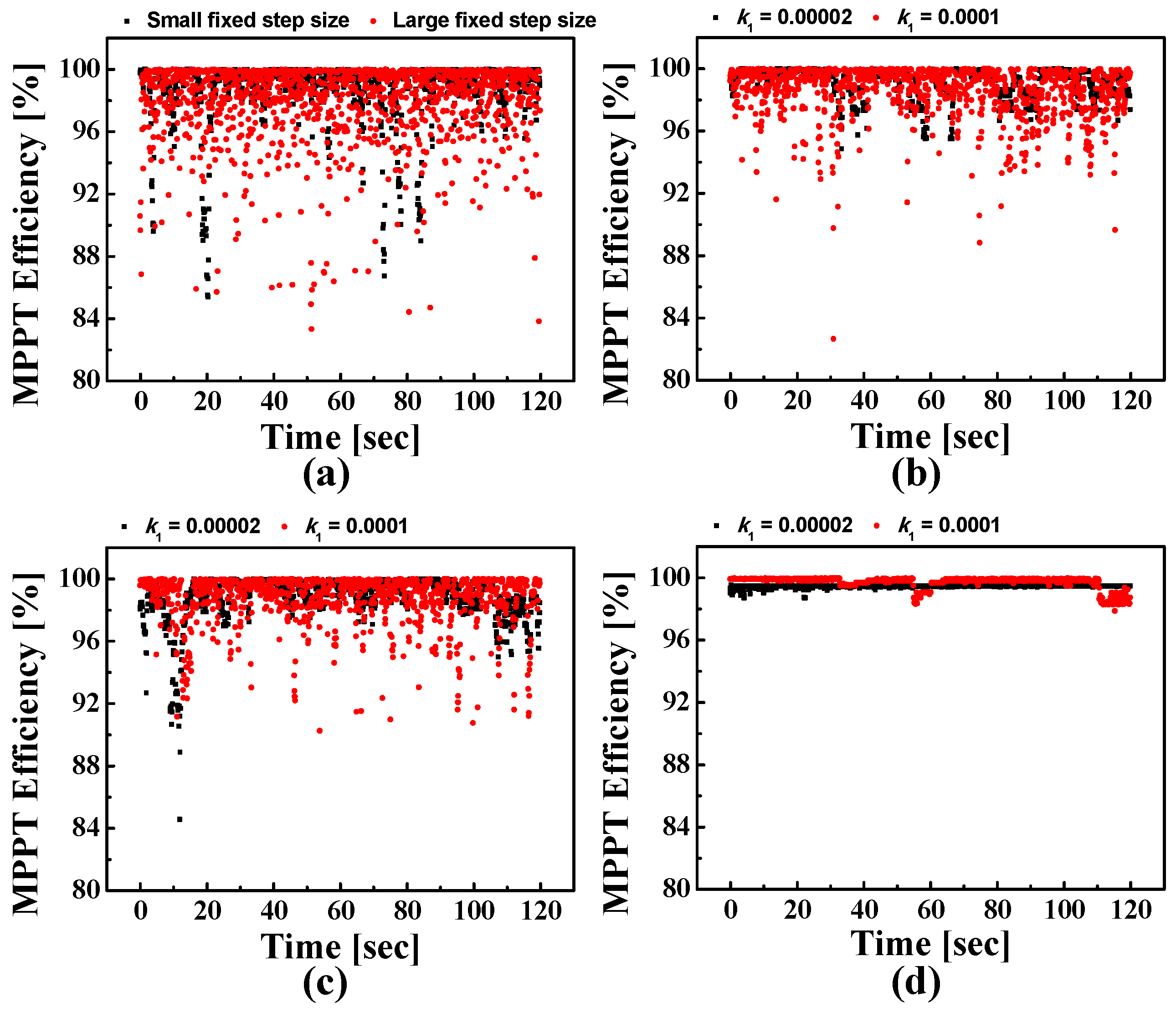
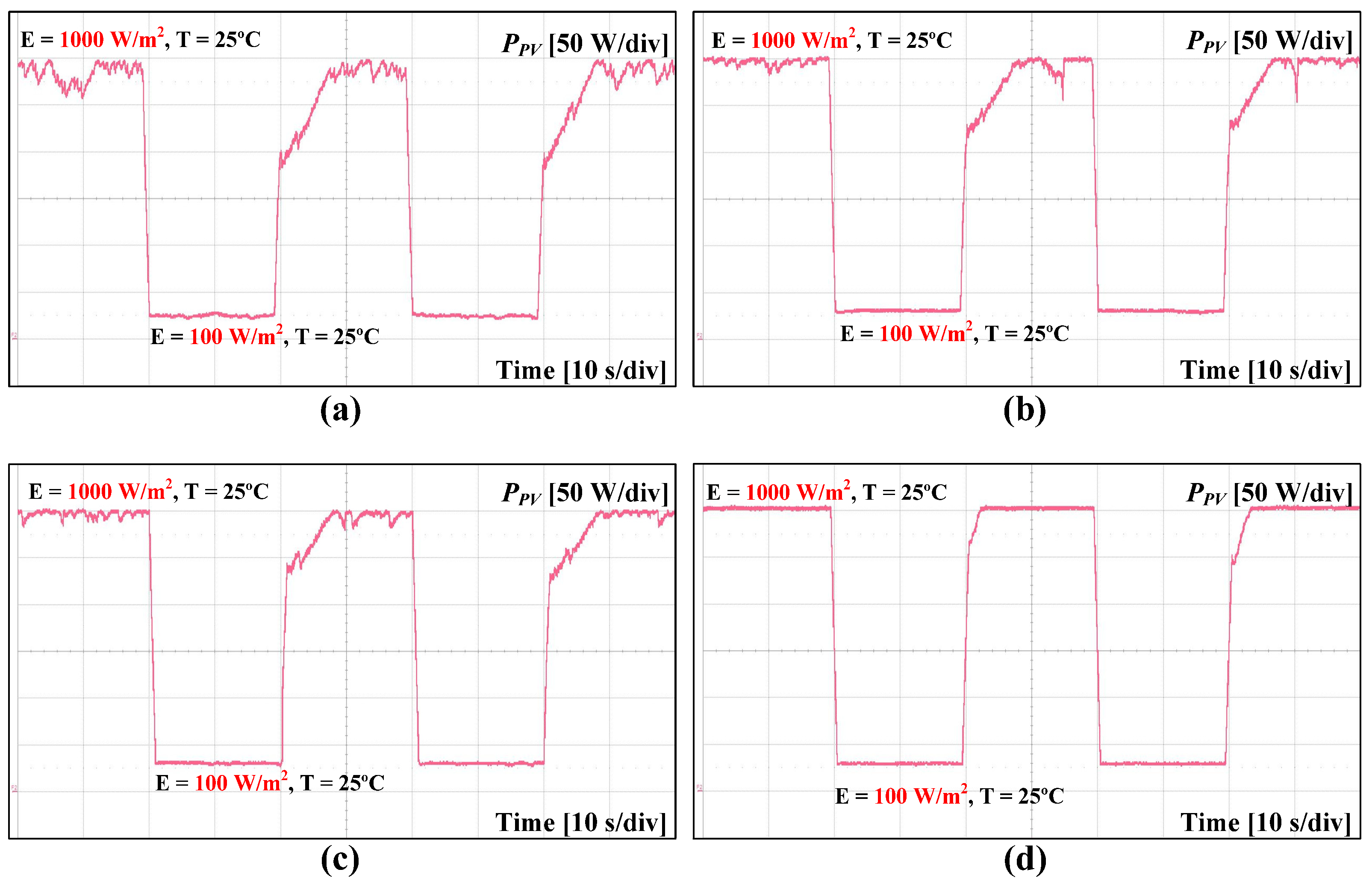
3.1. Experimental Results

Figure 12 shows the equipment settings to evaluate the performances of the MPPT algorithms. The output cable of the PV simulator (ETS60 from AMETEK Inc.) is connected to the input of the DC–DC converter (boost half-bridge topology), and the LAN cable of the PV simulator is connected to the notebook computer to set the characteristic curve (Figure 13) of the commercial 300-W PV module (Q.PEAK-G4.1 300 from Hanwha Inc.). Here, according to the irradiance level (E) and the module temperature (T), the electrical characteristics of the PV module “Q.PEAK-G4.1 300” are listed in Table 4. The output of the DC–DC converter is connected to the electronic load (DL1000H from NF Corp.) to consume the energy, and the notebook computer is connected to the DSP (TMS320F28335 from Texas Instruments Inc.) in the DC–DC converter by USB cable. The power meter (PW3336, from HIOKI Inc.) is used to measure the voltage (VPV), current (IPV), and power (PPV) of the PV simulator. Based on the sensed VPV and IPV, the DSP runs the MPPT algorithm and generates the gate signals (vgs1, vgs2) for operating the DC–DC converter. To compare the dynamic and energy utilization performances of the MPPT algorithms, four experiments were performed as follows.
First, the proposed MPPT algorithm and the conventional MPPT algorithms including a basic P&O of [21], an adaptive P&O of [26], and an adaptive INC of [27] were tested at the STC of E = 1000 W/m2 and T = 25 °C. Figure 14 shows the measured VPV, IPV, and PPV waveforms of the PV module when each MPPT algorithm is applied to a DC–DC converter. The basic P&O algorithm with a small fixed step size tracked the maximum power point (MPP) slowly, but it had small oscillations after reaching the MPP (Figure 14a). When the fixed step size increased, the tracking speed of the basic P&O algorithm increased as well, but the oscillations also increased (Figure 14b). To solve the problem of the fixed step size, the adaptive P&O and adaptive INC algorithms used a variable step size proportional to k1·ΔPPVVPV. However, these algorithms still had the oscillations at the MPP because the ΔPPVVPV is easily affected by sensing and calculation errors, sensing noise, and the ripples of VPV and IPV (Figure 14c–f). If the coefficient k1 is smaller, the oscillations at the MPP decreases, but the tracking speed is slower. To improve the problems of the previous MPPT algorithms mentioned above, the proposed MPPT algorithm uses two methods that can apply the optimal step size to each operating range. In the operating range near the MPP, a small fixed step size is used to minimize the oscillations at the MPP, but in the operating range far from the MPP, a variable step size proportional to k1·ΔPPVVPV is used to achieve fast tracking speed. The proposed MPPT algorithm can adjust the tracking speed using k1 so that it can track the MPP quickly. As a result, the proposed MPPT algorithm tracked the MPP with faster tracking speed and had smaller oscillations at the MPP when compared with the conventional algorithms (Figure 14g,h).
The MPPT efficiencies of the proposed and conventional MPPT algorithms were measured for two minutes after reaching the MPP under the same conditions as in Figure 14 (Figure 15). When a large fixed step size was applied, the basic P&O algorithm had the lowest average MPPT efficiency of 97.8% due to the largest oscillations at the MPP (Figure 15a). The adaptive P&O and adaptive INC algorithms with high k1(=0.0001) had higher average MPPT efficiencies of 98.5% and 98.7% than that of the basic P&O algorithm because they used variable step sizes (Figure 15b,c). In addition, the adaptive P&O and adaptive INC algorithms had higher average MPPT efficiencies of 99.1% and 98.9% than 98.7% of the basic P&O algorithm when small fixed step size and low k1(=0.00002) were applied. The proposed MPPT algorithm had the highest average MPPT efficiencies of 99.4% and 99.7% at low k1(=0.00002) and high k1(=0.0001) because it had the smallest oscillations at the MPP (Figure 15d).
The PPV waveforms were measured to compare the performances of the proposed and conventional MPPT algorithms when irradiance level changed abruptly from 1000 W/m2 to 100 W/m2 or from 100 W/m2 to 1000 W/m2 at a constant temperature of 25 °C (Figure 16). In each MPPT algorithm, the fixed step size and k1 were optimized by considering the trade-off between the tracking speed and the oscillations under the given conditions. When irradiance level changed from 100 W/m2 to 1000 W/m2, the basic P&O algorithm tracked the MPP within 20 s but had large oscillations (Figure 16a). The adaptive P&O and adaptive INC algorithms also tracked the MPP within 20 s, but they still had oscillations (Figure 16b,c). As shown in Figure 14c–f, these algorithms could reduce the oscillations using a small fixed step size or k1, but the tracking was slower. The proposed MPPT algorithm had no trade-off between the tracking speed and the oscillations because it uses a variable step size proportional to k1·ΔPPVVPV in the operating range far from the MPP and a small fixed step size in the operating range near the MPP. Therefore, when the irradiance level changed from 100 W/m2 to 1000 W/m2, the proposed MPPT algorithm showed smaller oscillations and faster tracking speed than other algorithms (Figure 16d).
Figure 17 shows the PPV waveforms measured to compare the performances of the proposed and conventional MPPT algorithms when the temperature changed abruptly from 15 °C to 75 °C or from 75 °C to 15 °C at a constant irradiance of 700 W/m2. In each MPPT algorithm, the fixed step size and k1 were optimized by considering the trade-off between the tracking speed and the oscillations under the given conditions. The basic P&O algorithm slowly tracked the MPP due to the fixed step size when the temperature changed from 75 °C to 15 °C (Figure 17a). The adaptive P&O and adaptive INC algorithms tracked the MPP faster than the basic P&O, but they still had oscillations after reaching the MPP (Figure 17b,c). The proposed MPPT algorithm not only had the fastest tracking speed but also had the smallest oscillations after reaching the MPP because it had no trade-off between the tracking speed and the oscillations (Figure 17d). The above results of the comparison experiments are summarized in Table 5.

3.2. Discussion

Among many MPPT algorithms, the P&O method was widely used due to its simple principle and ease of implementation. However, the basic P&O algorithm of [21] had a trade-off between tracking speed and oscillations due to a fixed step size (Figure 14a,b). To solve this problem, the adaptive P&O and adaptive INC algorithms using a variable step size were introduced [26,27]. These adaptive MPPT algorithms can reduce the oscillations at the MPP because the variable step size is automatically adjusted according to the slope (ΔPPVVPV) of the P–V curve (Figure 14c–f). However, the adaptive MPPT algorithms still had oscillations after reaching the MPP because the calculated ΔPPVVPV is easily affected by sensing and calculation errors, sensing noise, and the ripples of VPV and IPV. To improve the performances of the conventional MPPT algorithms mentioned above, the proposed MPPT algorithm used a small fixed step size in operating range near the MPP and a variable step size proportional to k1∙ΔPPVVPV in operating range far from the MPP. As a result, the proposed MPPT algorithm had higher MPPT efficiency than the conventional MPPT algorithms (Figure 15) and showed faster tracking speed and smaller oscillations under dynamic weather conditions (Figure 16 and Figure 17). These advantages of the proposed MPPT algorithm enable the distributed PV system to operate at its maximum performance, regardless of weather conditions.

4. Conclusions

In this paper, an advanced MPPT algorithm for distributed PV systems was proposed. The proposed MPPT algorithm improved the MPPT accuracy and dynamic response of the conventional MPPT algorithms by using two methods that can apply the optimal step size to each operating range. In the operating range near the MPP, a small fixed step size is used to minimize the oscillations at the MPP, but in the operating range far from the MPP, a variable step size proportional to k1·ΔPPVVPV is used to achieve fast tracking speed. These advantages of the proposed MPPT algorithm were verified by comparison with the conventional MPPT algorithms: a basic P&O algorithm with fixed step size, an adaptive P&O algorithm with variable step size, and an adaptive INC algorithm with a variable step size. In the experimental results, the proposed MPPT algorithm had the highest MPPT efficiency of 99.7% compared with the conventional MPPT algorithms. In addition, it showed the fastest tracking speed and smallest oscillations under abruptly changing irradiance levels and temperature conditions. Due to these advantages of the proposed MPPT algorithm, the PV systems using the proposed MPPT algorithm can produce more electrical energy than that using the conventional MPPT algorithms. Moreover, the proposed MPPT algorithm requires low computational load of DSP because the formulas used for step size are simple, which is a good advantage in terms of user convenience and cost that are important for commercialization. As a result, the proposed MPPT algorithm is well-suited for distributed PV systems requiring high MPPT efficiency and fast dynamic response.

Author Contributions

Both authors contributed equally to this work. H.-S.L. presented the main idea of the MPPT algorithm. H.-S.L. and J.-J.Y. analyzed the proposed MPPT algorithm and performed experiments. J.-J.Y. contributed to the overall composition and writing of the manuscript.

Funding

This work was supported by the National Research Foundation of Korea (NRF) grant funded by the government of Korea (MSIP) (NRF-2018R1A1A1A05079496). This research was also supported by the Korea Electric Power Corporation (Grant number: R17XA05-15).

Conflicts of Interest

The authors have no conflict of interest.

References

  1. Malinowski, M.; Leon, J.I.; Abu-Rub, H. Solar photovoltaic and thermal energy systems: Current technology and future trends. Proc. IEEE 2017, 105, 2132–2146. [Google Scholar] [CrossRef]
  2. Kroposki, B.; Johnson, B.; Zhang, Y.; Gevorgian, V.; Denholm, P.; Hodge, B.M.; Hannegan, B. Achieving a 100% renewable grid: Operating electric power systems with extremely high levels of variable renewable energy. IEEE Power Energy Mag. 2017, 15, 61–73. [Google Scholar] [CrossRef]
  3. García-Rodríguez, L. Renewable Energy Applications in Desalination: State of the Art. Sol. Energy 2003, 75, 381–393. [Google Scholar] [CrossRef]
  4. Renewables 2019 Global Status Report, Renewable Energy Policy Network for the 21st Century (REN21). 2019. Available online: https://www.ren21.net/gsr-2019/ (accessed on 2 September 2019).
  5. Romero-Cadaval, E.; Francois, B.; Malinowski, M.; Zhong, Q.C. Grid-connected photovoltaic plants: An alternative energy source, replacing conventional sources. IEEE Ind. Electron. Mag. 2015, 9, 18–32. [Google Scholar] [CrossRef]
  6. Zhao, P.; Suryanarayanan, S.; Simoes, M.G. An energy management system for building structures using a multi-agent decision-making control methodology. IEEE Trans. Ind. Appl. 2013, 49, 322–330. [Google Scholar] [CrossRef]
  7. Strunz, K.; Abbasi, E.; Huu, D.N. DC microgrid for wind and solar power integration. IEEE J. Emerg. Sel. Top. Power Electron. 2014, 2, 115–126. [Google Scholar] [CrossRef]
  8. Feldman, D.; Barbose, G.; Margolis, R.; Bolinger, M.; Chung, D.; Fu, R.; Seel, J.; Davidson, C.; Darghouth, N.; Wiser, R. Photovoltaic System Pricing Trends Historical, Recent, and Near-Term Projections 2015 Edition. Available online: https://escholarship.org/content/qt9pc3x32t/qt9pc3x32t.pdf (accessed on 2 September 2019).
  9. Zsiborács, H.; Hegedűsné Baranyai, N.; Csányi, S.; Vincze, A.; Pintér, G. Economic Analysis of Grid-Connected PV System Regulations: A Hungarian Case Study. Electronics 2019, 8, 149. [Google Scholar] [CrossRef]
  10. Camera, F.L. Renewable Power Generation Costs in 2018; International Renewable Energy Agency (IRENA): Abu Dhabi, UAE, 2019; Available online: https://www.irena.org/publications/2019/May/Renewable-power-generation-costs-in-2018 (accessed on 2 September 2019).
  11. Meza, C.; Negroni, J.J.; Biel, D.; Guinjoan, F. Energy-balance modeling and discrete control for single-phase grid-connected PV central inverters. IEEE Trans. Ind. Electron. 2008, 55, 2734–2743. [Google Scholar] [CrossRef]
  12. Flicker, J.; Tamizhmani, G.; Moorthy, M.K.; Thiagarajan, R.; Ayyanar, R. Accelerated testing of module-level power electronics for longterm reliability. IEEE J. Photovolt. 2017, 7, 259–267. [Google Scholar] [CrossRef]
  13. Liu, Y.H.; Chen, J.H.; Huang, J.W. A review of maximum power point tracking techniques for use in partially shaded conditions. Renew. Sustain. Energy Rev. 2015, 41, 436–453. [Google Scholar] [CrossRef]
  14. Gu, B.; Dominic, J.; Lai, J.S.; Zhao, Z.; Liu, C. High boost ratio hybrid transformer DC-DC converter for photovoltaic module applications. IEEE Trans. Power Electron. 2013, 28, 2048–2058. [Google Scholar] [CrossRef]
  15. Sinapis, K.; Tzikas, C.; Litjens, G.; Van den Donker, M.; Folkerts, W.; Van Sark, W.G.J.H.M.; Smets, A. A comprehensive study on partial shading response of c-Si modules and yield modeling of string inverter and module level power electronics. Sol. Energy 2016, 135, 731–741. [Google Scholar] [CrossRef] [Green Version]
  16. Aganza-Torres, A.; Cardenas, V.; Pacas, M.; Gonzales, M. An efficiency comparative analysis of isolated multi-source grid-connected PV generation systems based on a HF-link micro-inverter approach. Sol. Energy 2016, 127, 239–249. [Google Scholar] [CrossRef]
  17. Luo, H.; Wen, H.; Li, X.; Jiang, L.; Hu, Y. Synchronous buck converter based low-cost and high-efficiency sub-module DMPPT PV system under partial shading conditions. Energy Convers. Manag. 2016, 126, 473–487. [Google Scholar] [CrossRef]
  18. Femia, N.; Lisi, G.; Petrone, G.; Spagnuolo, G.; Vitelli, M. Distributed maximum power point tracking of photovoltaic arrays: Novel approach and system analysis. IEEE Trans. Ind. Electron. 2008, 55, 2610–2621. [Google Scholar] [CrossRef] [Green Version]
  19. Wang, F.; Fang, Z.; Lee, F.C.; Zhu, T.; Yi, H. Analysis of existence-judging criteria for optimal power regions in DMPPT PV systems. IEEE Trans. Energy Convers. 2016, 31, 1433–1441. [Google Scholar] [CrossRef]
  20. Ahmed, A.; Ran, L.; Bumby, J. Perturbation parameters design for hill climbing MPPT techniques. In Proceedings of the IEEE International Symposium on Industrial Electronics, Hangzhou, China, 28–31 May 2012. [Google Scholar] [CrossRef]
  21. Hua, C.; Lin, J.; Shen, C. Implementation of a DSP-controlled photovoltaic system with peak power tracking. IEEE Trans. Ind. Electron. 1998, 45, 99–107. [Google Scholar] [CrossRef] [Green Version]
  22. Veerachary, M.; Senjyu, T.; Uezato, K. Voltage-based maximum power point tracking control of PV system. IEEE Trans. Aerosp. Eelctron. Syst. 2002, 38, 262–270. [Google Scholar] [CrossRef] [Green Version]
  23. Femia, N.; Petrone, G.; Spagnuolo, G.; Vitelli, M. Optimization of perturb and observe maximum power point tracking method. IEEE Trans. Power Electron. 2005, 20, 963–973. [Google Scholar] [CrossRef]
  24. Safari, A.; Mekhilef, S. Simulation and hardware implementation of incremental conductance MPPT with direct control method using cuk converter. IEEE Trans. Ind. Electron. 2011, 58, 1154–1161. [Google Scholar] [CrossRef]
  25. Xiao, W.; Dunford, W.G. A modified adaptive hill climbing MPPT method for photovoltaic power systems. In Proceedings of the IEEE 35th Annual Power Electronics Specialists Conference, Aachen, Germany, 20–25 June 2004. [Google Scholar] [CrossRef]
  26. Zhang, X.; Zhang, H.; Zhang, H.; Zhang, P.; Wang, F.; Jia, H.; Song, D. A variable step-size P&O method in the application of MPPT control for a PV system. In Proceedings of the IEEE Advanced Information Management, Communicates, Electronic and Automation Control Conference (IMCEC), Xi’an, China, 3–5 October 2016. [Google Scholar] [CrossRef]
  27. Liu, F.; Duan, S.; Liu, F.; Liu, B.; Kang, Y. A variable step size INC MPPT method for PV systems. IEEE Trans. Ind. Electron. 2008, 55, 2622–2628. [Google Scholar] [CrossRef]
  28. Pandey, A.; Dasgupta, N.; Mukerjee, A.K. High-performance algorithms for drift avoidance and fast tracking in solar MPPT system. IEEE Trans. Energy Convers. 2008, 23, 681–689. [Google Scholar] [CrossRef]
  29. Aashoor, F.A.O.; Robinson, F.V.P. A Variable Step Size Perturb and Observe Algorithm for Photovoltaic Maximum Power Point Tracking. In Proceedings of the 47th International Universities Power Engineering Conference (UPEC), London, UK, 4–7 September 2012. [Google Scholar] [CrossRef]
  30. Macaulay, J.; Zhou, Z. A fuzzy logical-based variable step size P&O MPPT algorithm for photovoltaic system. Energies 2018, 11, 1340. [Google Scholar] [CrossRef]
  31. Chen, Y.T.; Jhang, Y.C.; Liang, R.H. A fuzzy-logic based auto-scaling variable step-size MPPT method for PV systems. Sol. Energy 2016, 126, 53–63. [Google Scholar] [CrossRef]
  32. Harrag, A.; Messalti, S. Variable step size modified p&o mppt algorithm using ga-based hybrid offline/online pid controller. Renew. Sustain. Energy Rev. 2015, 49, 1247–1260. [Google Scholar] [CrossRef]
  33. Villalva, M.G.; Gazoli, J.R.; Filho, E.R. Comprehensive approach to modeling and simulation of photovoltaic arrays. IEEE Trans. Power Electron. 2009, 24, 1198–1208. [Google Scholar] [CrossRef]
  34. Shongwe, S.; Hanif, M. Comparative analysis of different singlediode PV modeling methods. IEEE J. Photovolt. 2015, 5, 938–946. [Google Scholar] [CrossRef]
Figure 1. Block diagrams of (a) the central inverter and (b) the module-level power electronics.
Energies 12 03576 g001
Figure 2. Principle of operation for the hill-climbing and perturb and observe (P&O) algorithms.
Energies 12 03576 g002
Figure 3. Principle of operation for the incremental conductance (INC) algorithm.
Energies 12 03576 g003
Figure 4. Flow chart of the genetic algorithm.
Energies 12 03576 g004
Figure 5. Diagram of the distributed photovoltaic (PV) system with maximum power point tracking (MPPT) algorithm.
Energies 12 03576 g005
Figure 6. Equivalent circuit of the PV module.
Energies 12 03576 g006
Figure 7. (a) Current–voltage characteristic curve and (b) power–voltage characteristic curve of the PV module.
Energies 12 03576 g007
Figure 8. Diagrams of (a) the micro-inverter and (b) the direct current (DC)-optimizer.
Energies 12 03576 g008
Figure 9. Principle of operation for the proposed MPPT algorithm.
Energies 12 03576 g009
Figure 10. Flow chart of the proposed MPPT algorithm.
Energies 12 03576 g010
Figure 11. The process for generating a duty ratio (D) in the digital signal processor (DSP).
Energies 12 03576 g011
Figure 12. (a) Photograph and (b) block diagram of the equipment settings for experiments to evaluate the MPPT performance.
Energies 12 03576 g012
Figure 13. Electrical characteristic curve of a 300 W PV module “Q.PEAK-G4.1 300” under the standard test conditions (STC) of irradiance level of 1000 W/m2 and module temperature of 25 °C.
Energies 12 03576 g013
Figure 14. Voltage (VPV), current (IPV), and power (PPV) waveforms of the PV module measured using the basic P&O algorithm with (a) small fixed step size or (b) large fixed step size, using the adaptive P&O algorithm with (c) low k1(=0.00002) or (d) high k1(=0.0001), using the adaptive INC algorithm with (e) low k1(=0.00002) or (f) high k1(=0.0001), and using the proposed MPPT algorithm with (g) low k1(=0.00002) and small fixed step size or (h) high k1(=0.0001) and small fixed step size.
Energies 12 03576 g014
Figure 15. Measured MPPT efficiencies of (a) the basic P&O with small or large fixe step sizes, (b) the adaptive P&O with low k1(=0.00002) or high k1(=0.0001), (c) the adaptive INC with low k1(=0.00002) or high k1(=0.0001), and (d) the proposed MPPT algorithms with low k1(=0.00002) or high k1(=0.0001).
Energies 12 03576 g015
Figure 16. Power (PPV) waveforms of the PV module measured using (a) the basic P&O algorithm, (b) the adaptive P&O algorithm, (c) the adaptive INC algorithm, and (d) the proposed MPPT algorithm under abruptly changing irradiance conditions.
Energies 12 03576 g016
Figure 17. Power (PPV) waveforms of the PV module measured using (a) the basic P&O algorithm, (b) the adaptive P&O algorithm, (c) the adaptive INC algorithm, and (d) the proposed MPPT algorithm under abruptly changing temperature conditions.
Energies 12 03576 g017
Table 1. Methodology of the hill-climbing and P&O algorithms.
ConditionsActions
(i) ΔPPV < 0 and ΔVPV < 0Duty decrease
(ii) ΔPPV > 0 and ΔVPV > 0Duty decrease
(iii) ΔPPV > 0 and ΔVPV < 0Duty increase
(iv) ΔPPV < 0 and ΔVPV > 0Duty increase
(v) ΔPPV = 0 and ΔVPV = 0No action
Table 2. Methodology of the INC algorithm.
ConditionsActions
(i) –ΔIPVVPV < IPV/VPV and ΔIPV > 0Duty decrease
(ii) –ΔIPVVPV < IPV/VPV and ΔIPV < 0Duty decrease
(iii) –ΔIPVVPV > IPV/VPV and ΔIPV > 0Duty increase
(iv) –ΔIPVVPV > IPV/VPV and ΔIPV < 0Duty increase
(v) –ΔIPVVPV = IPV/VPV and ΔIPV = 0No action
Table 3. Rule-based lookup table based on the fuzzy logic.
ΔIPVΔPPV
NBNSZOPSPB
NBNBNSNSZOZO
NSNSZOZOZOPS
ZOZOZOZOPSPS
PSZOPSPSPSPB
PBPSPSPBPBPB
Table 4. Electrical characteristics of the PV module “Q.PEAK-G4.1 300” at different irradiance levels (E) and module temperatures (T).
ConditionsOpen-Circuit Voltage (VOC)Short-Circuit Current (ISC)Voltage at MPP (VMPP)Current at MPP (IMPP)Power at MPP (PMPP)
E = 1000 W/m2 and T = 25 °C39.76 V9.77 A33.11 V9.082 A300.71 W
E = 100 W/m2 and T = 25 °C35.78 V1.086 A29.8 V1.009 A30.07 W
E = 700 W/m2 and T = 15 °C40.24 V7.021 A33.51 V6.527 A218.72 W
E = 700 W/m2 and T = 75 °C33.66 V6.502 A28.04 V6.044 A169.47 W
Table 5. Comparisons between the proposed and conventional MPPT algorithms.
Performance ParametersBasic P&O Algorithm of [21]Adaptive P&O Algorithm of [26]Adaptive INC Algorithm of [27]Proposed Algorithm
Implementation complexitysimplemediummediummedium
MPPT methodfixed step size (k2Vstep) in whole operating rangevariable step size (k1VstepΔPPVVPV) in whole operating rangevariable step size (k1VstepΔPPVVPV) in whole operating rangesmall fixed step size (k2Vstep) near the MPP,
variable step size (k1VstepΔPPVVPV) far from the MPP
MPPT efficiency97.8%98.5%98.7%99.7%
Performance at rapid change of irradiancepoormediummediumgood
Performance at rapid change of temperaturepoormediummediumgood
Speedfastfastfastfast
Accuracylowmediummediumhigh

