Transient Stress Distribution and Failure Response of a Wellbore Drilled by a Periodic Load

Abstract

The poroelastodynamic failure of a wellbore due to periodic loading during drilling is an unsolved problem. The conventional poroelastic method to calculate the stress distribution around wellbore is for static loading cases and cannot be used for short-time dynamic-loading cases which result in wave propagation in the formation. This paper formulates a poroelastodynamic model to characterize dynamic stress and pressure wave due to periodic loadings and to analyze the transient failure of the suddenly drilled wellbore in a non-hydrostatic stress field. The fully coupled poroelastodynamic model was developed based on the equations of motion, fluid flow and constitutive equations to reflect stress and pressure waves that resulted from a periodic stress perturbation at the wellbore surface. The model was analytically solved by means of field expansions of the solutions, by performing a Laplace transform as well as some special techniques. Simulation results show that the pressure and stress responses inside the formation resemble a damped oscillator where the amplitude decays as the distance to wellbore increases. Especially the potential shear failure zone around the wellbore was computed and plotted. Influences of poroelastic parameters, in-situ stress and periodic load parameters on the shear failure responses were analyzed in a detailed parametric study, and the results provide fundamental insights into wellbore stability maintenance in different reservoirs.

1. Introduction

Wellbore instability can cause many substantial problems during drilling, such as stuck pipe and lost circulation. Overall, problems related to wellbore collapse account for 5–10% of drilling costs in exploration and production, which are hundreds of million dollars per year, when considering time loss and the rental of drilling equipment [1]. Drilling a wellbore in a formation results in the redistribution of the stress around the borehole. The maximum compressive stress usually occurs as the hoop stress at the wellbore surface in the direction of the minimum principal stress. When the shear stress exceeds the shear strength of the rock near the wellbore, shear failure happens. If the failed rock exceeds the cleaning capacity of the mud circulation, the excessive failed rock can cause stuck drill pipe or bottom-hole assembly. Sometimes, wellbore collapse can result in sidetracked holes and abandoned wells, which means a great loss in oil and gas industry. Therefore, wellbore stability analysis is vital to safe and effective drilling and production. Wellbore stability analysis requires the information on stress distribution around the wellbore.

Study on stress distribution around a wellbore can be traced back to the Kirsch solution [2], which is used to calculate the stress distribution near a circular hole in an infinite plate. Based on Kirsch’s work, Bradley [3] presented an analytical solution of wellbore stress distribution. This solution is used as the standard approach to obtain stress distribution by researchers [1,4,5]. However, it can only be used for static loading analyses. Several commonly used failure criteria for wellbore collapse have also been developed, such as Mohr-Coulomb failure criterion, Modified Lade failure criterion, von Mises criterion and Drucker-Prager failure criterion [1]. In fact, loadings inside the wellbore are more often dynamic than static. The periodic loads applied at the borehole surface during drilling can generate stress and pressure waves. In this regard, the inertial effect of the solid-fluid system has to be taken into account [6]. Detournay and Cheng [7] proposed an analytical method for calculation of wellbore stress distribution considering poroelastic effect and studied the failure initiation on the basis of stress distribution. Zamanipour et al. [8] investigated the wellbore stress distribution and wellbore stability when transient surge stress is generated in a directional wellbore during tripping process. Zhang et al. [9] conducted wellbore stability analysis by coupling transient swab/surge model and poromechanical solution during tripping and reaming processes and proposed a work flow to obtain safe mud-weight window. Meng et al. [10] developed a coupled poroelastodynamic model to obtain dynamic stress distribution around the wellbore.

One of the salient features of the poroelastic response is the generation and dissipation of excess pore water pressure under applied loadings, and wave propagation is induced from various external disturbances such as periodic surge/swab pressure during drilling [11,12]. Biot developed the theory of wave propagation in poroelastic materials by adding the inertia terms to his three-dimensional consolidation theory [13,14,15]. Over the past decades, Biot’s theory of poroelastodynamics has been used by many researchers and the scientific groundwork for the model has been more firmly established through some experimental validations of its most fundamental predictions [16,17,18]. A detailed review on formulation and development of Biot’s theory of poroelastodynamics with some analytical solutions can be found in [19].

An important class of problems encountered in dynamic response of using poroelastodynamics is related to the study of wave propagation from an underground borehole. However, some studies on the poroelastodynamics are limited to axisymmetric cases, thus, the problems can be simplified to one dimension (1D) [20,21,22]. In reality, the original formation is subjected to a non-hydrostatic stress field and the stress release at the wellbore surface after drilling includes radial and shear stress. The early 1D simplification is incapable of analyzing the shear stress wave propagation in the formation so that it limits the application of the poroelastodynamic model in the engineering field. Two-dimensional (2D) problems are also investigated by a few researchers in recent years. Liu et al. [23] theoretically investigated the scattering of an elastic wave by a cylindrical shell embedded in a poroelastic medium. They employed the normal mode expansion technique for analyzing the scattering field. Hasheminejad and Kazemirad [24] studied the dynamic response of a permeable circular tunnel lining of circumferentially varying wall thickness buried in an unbounded porous elastic fluid-saturated formation. Particularly, they studied the two-dimensional dynamic interaction of monochromatic progressive plane compressional and shear seismic waves. They used the Helmholtz decomposition theorem to resolve the displacement fields as a superposition of longitudinal and transverse vector components. Xia et al. [25] presented an exact closed-form solution for poroelastodynamic response of a borehole in a non-hydrostatic stress field and the solution was decomposed into an axisymmetric mode and an asymmetric mode. However, they considered a constant pressure at the wellbore surface and the shear failure response was not analyzed.

More recently, Senjuntichai et al. [26] used poroelastodynamic model to investigate three-dimensional (3D) dynamic response of a multilayered poroelastic medium subjected to time-harmonic loading in Cartesian coordinate system. Keawsawasvong and Senjuntichai [27] presented dynamic fundamental solutions of a transversely isotropic poroelastic half-plane subjected to time harmonic buried loads and fluid sources. In drilling engineering, a periodic load during drilling is a common occurrence. Although the equations of poroelastodynamics were put forward by Biot very early, it is still challenging to study the transient responses of a wellbore subjected to a non-hydrostatic in-situ stress field and a periodic load during drilling. The problem becomes the superposition of an axisymmetric mode and an asymmetric mode, and the periodic boundary condition further amplifies the complexity of the problem. To the best of our knowledge, this challenge has not been addressed directly.

In this paper, we consider the poroelastodynamic failure of a wellbore due to periodic loading during drilling; the wellbore is embedded into a formation that is characterized by non-hydrostatic horizontal far-field stresses. The poroelastodynamic model is developed based on Biot’s theory, and we present a novel solution to the model. The stress and pressure waves in the formation resulted from a periodic stress perturbation at the wellbore surface are analyzed in detail, and the results show that the pressure and stress responses inside the formation resemble a damped oscillator where the amplitude decays as the distance to wellbore increases. It is noteworthy that the pore pressure reaches its peak at a certain time and location, while the conventional poroelastic theory always fails to discover this phenomenon due to the lack of consideration of solid-fluid acceleration. The shear failure response has also been studied. Finally, the influences of poroelastic parameters, in-situ stress and periodic load parameters on the shear failure responses are analyzed in a detailed parametric study. The model and results presented in this paper provide fundamental insights into wellbore instability in different reservoirs, and suggestions are made on maintaining wellbore stability.

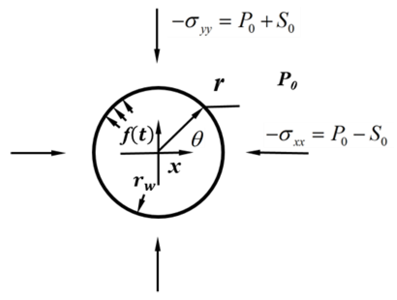
2. Mathematical Formulation

To find the governing equations for transient response of a wellbore subjected to dynamic loadings, a fundamental knowledge of poroelastodynamics is required. In this section, we consider a vertical borehole drilled in a poroelastic formation characterized by non-hydrostatic horizontal far-field stresses, and a periodic load is applied at the borehole surface, as shown in Figure 1. The definitions of all the symbols that have physical meanings are given in

Table A1. List of symbols and definitions.

Symbol	Unit	Definition
$r$	m	Radius defined in Figure 1
$\theta$		Angle defined in Figure 1
$r_w$	m	Radius of the borehole
$P_0$, $S_0$	MPa	Far-field mean and deviatoric parts of the stress
$u_r$, $u_{\theta }$	m	Displacement components of the solid
$w_r$, $w_{\theta }$	m	Displacement components of the fluid
${\sigma }_{ij}$	MPa	Stress component
${\sigma }_{rr}$, ${\sigma }_{\theta \theta }$, ${\sigma }_{r\theta }$	MPa	Radial stress, hoop stress and shear stress
$e_{ij}$		Strain component
$e$		Volumetric strain
$p$	MPa	Excess pore water pressure
$p_w$	MPa	Constant bottom-hole pressure
$p_h$	MPa	Transient bottom-hole pressure
${\delta }_{ij}$		Kronecker delta. ${\delta }_{ij}=1$ when $i=j$ and ${\delta }_{ij}=0$ when $i\ne j$
$\lambda$	GPa	Lame constant of the bulk material
$\mu$	GPa	Shear modulus of the bulk material
$\zeta$		Increment of pore fluid per unit volume
$\alpha$		Biot effective stress coefficient
$M$	GPa	Biot modulus
$K_s$	GPa	Bulk modulus of solid grains
$K_f$	GPa	Bulk modulus of pore fluid
$K$	GPa	Drained bulk modulus of the porous medium
$\rho$	Kg·m−3	Density of porous medium
${\rho }_f$	Kg·m−3	Density of porous fluid
$t$	s	Time
$V$, $V_s$, $V_p$	m3	Volumes of the porous medium, solid grains and pores
$\sigma ’$	MPa	Effective stress vector of the porous medium
$q_w$	m3·s−1·m−2	Volumetric flux of pore fluid
${\rho }_a$	Kg·m−3	Mass density of the fluid added into the porous medium
$\varphi$		Porosity of the porous medium
$\kappa$	mD(10−15m2)	Permeability of the porous medium
$\tau$	mPa·s	Viscosity of the porous fluid
$p_0$	MPa	Unperturbed pore pressure
$2L$	MPa	Amplitude of stress wave
$\omega$	s−1	Angular frequency of stress wave
$\phi$	°	Internal friction angle
$C_t$	MPa	Cohesion
${\sigma }_H$	MPa	Maximum principal stress
${\sigma }_h$	MPa	Minimum principal stress
$a$		Non-dimensional tortuosity factor
$\eta$, ${\overline{\mathsf{\Omega }}}_1,{\overline{\mathsf{\Omega }}}_2$ ${\overline{\mathsf{\Phi }}}_1,{\overline{\mathsf{\Phi }}}_2,{\overline{\mathsf{\Phi }}}_3,{\overline{\mathsf{\Phi }}}_4$ ${\overline{\mathsf{\Psi }}}_1,{\overline{\mathsf{\Psi }}}_2,{\overline{\mathsf{\Psi }}}_3$		Dimensionless quantities
$A_n$, $B_n$, $C_n$		Constants in different mode solutions

in Appendix A. ${\sigma }_{yy}$ and ${\sigma }_{xx}$ are the maximum and minimum horizontal in-situ stresses, respectively. It should be noted that the directions of maximum and minimum horizontal in-situ stresses in the figures of stress or pore pressure distribution and figures of shear failure zone distribution are in accordance with Figure 1.

2.1. Constitutive and Dynamic Equations

Assuming the rock to be a linear-elastic, isotropic and saturated porous medium and considering the effect of deformation on the balance of mass, the constitutive equations for linear poroelasticity, could be written as follows (note that tension is here taken as positive) [7]:

$${\sigma }_{ij}=2\mu e_{ij}+\lambda e{\delta }_{ij}-\alpha p{\delta }_{ij}$$

(1)

$$p=M\left(\zeta -\alpha e\right)$$

(2)

where ${\sigma }_{ij}$ and $e_{ij}$ are the total stress and strain components, respectively; $e$ is the volumetric strain; $p$ is the excess pore water pressure; ${\delta }_{ij}$ is the Kronecker delta, which equals 1 when $i=j$ or equals 0 when $i\ne j$; $\lambda$ and $\mu$ are the Lame constants and $\mu$ is also called shear modulus; $\zeta$ is the increment of pore fluid per unit volume; $\alpha$ and $M$ are the Biot effective stress coefficient and Biot modulus, respectively, which have the relations $\alpha =1-K/K_s$ and $1/M=\varphi /K_f+\left(1-\varphi \right)/K_s$, where $K_s$ and $K_f$ are the bulk modulus of solid grains and pore fluid, respectively; $K=\lambda +2\mu /3$ is the drained bulk modulus of the porous medium. Compared to underground in-situ stress and pore pressure, body forces are negligible in the case studied. In the absence of body forces, the dynamic equations of motion can be written as [25]:

$$\frac{\partial {\sigma }_{rr}}{\partial r}+\frac{1}{r}\frac{\partial {\sigma }_{r\theta }}{\partial \theta }+\frac{{\sigma }_{rr}-{\sigma }_{\theta \theta }}{r}=\rho \frac{{\partial }^2{u}_r}{\partial t^2}+{\rho }_f\frac{{\partial }^2{w}_r}{\partial t^2}$$

(3)

$$\frac{1}{r}\frac{\partial {\sigma }_{\theta \theta }}{\partial \theta }+\frac{\partial {\sigma }_{r\theta }}{\partial r}+\frac{2{\sigma }_{r\theta }}{r}=\rho \frac{{\partial }^2{u}_{\theta }}{\partial t^2}+{\rho }_f\frac{{\partial }^2{w}_{\theta }}{\partial t^2}$$

(4)

where $\rho$ and ${\rho }_f$ are density of porous medium and fluid, respectively; $t$ is time; $r$ is radius defined in Figure 1; $u_r,u_{\theta },w_r,w_{\theta }$ are the displacement components of solid and fluid, respectively; ${\sigma }_{rr},{\sigma }_{\theta \theta },{\sigma }_{r\theta }$ are the radial stress, hoop stress and shear stress, respectively. The subscripts $r$ and $\theta$ refer to the radial and azimuthal components, respectively. Substituting Equation (1) and Equation (2) into Equation (3) and Equation (4), we have the governing equations in displacement form in polar coordinates:

$$\mu {\nabla }^2{u}_r-\frac{\mu }{r^2}\left(\frac{2\partial u_{\theta }}{\partial \theta }+u_r\right)+\left(\lambda +\mu \right)\frac{\partial e}{\partial r}-\alpha \frac{\partial p}{\partial r}=\rho {\ddot{u}}_r+{\rho }_f{\ddot{w}}_r$$

(5)

$$\mu {\nabla }^2{u}_{\theta }-\frac{\mu }{r^2}\left(u_{\theta }-\frac{2\partial u_r}{\partial \theta }\right)+\left(\lambda +\mu \right)\frac{\partial e}{r\partial \theta }-\alpha \frac{\partial p}{r\partial \theta }=\rho {\ddot{u}}_{\theta }+{\rho }_f{\ddot{w}}_{\theta }$$

(6)

It is noted that two “·” on top of a variable means the second derivative of the variable with respect to time and similarly, one “·” on top means the first derivative of the variable with respect to time.

2.2. Fluid Flow Equation

The rates of total changes of the porous medium with respect to time satisfy the following relationship:

$$\frac{1}{V}\frac{\partial V}{\partial t}=\frac{1}{V}\frac{\partial V_s}{\partial t}+\frac{1}{V}\frac{\partial V_p}{\partial t}=\frac{\partial e}{\partial t}$$

(7)

where $V,V_s,V_p$ are the volumes of the porous medium, solid grains and pores, respectively. The changes of volume of soil grains and pores are given by:

$$\frac{1}{V}\frac{\partial V_s}{\partial t}=-\frac{1-\varphi }{K_s}\frac{\partial p}{\partial t}+\frac{1}{3K_s}m\frac{\partial \sigma ’}{\partial t}$$

(8)

$$\frac{1}{V}\frac{\partial V_p}{\partial t}=-\nabla q_w-\frac{\varphi }{K_f}\frac{\partial p}{\partial t}$$

(9)

where $\mathbf{m}=\left[111000\right]$ and $\sigma ’={\sigma }_{ij}-\alpha p{\delta }_{ij}$ denotes the effective stress vector of the porous medium; $\varphi$ is the porosity of the porous medium; $q_w$ is the volumetric flux of pore fluid, which is the rate of volumetric flow across a unit area. Substituting the constitutive relation Equation (1) into Equation (8) gives:

$$\frac{1}{V}\frac{\partial V_s}{\partial t}=-\frac{1-\varphi }{K_s}\frac{\partial p}{\partial t}+\frac{K}{K_s}\frac{\partial e}{\partial t}$$

(10)

Substituting Equations (8)–(10) into Equation (7) yields:

$$\nabla q_w=-\alpha \frac{\partial e}{\partial t}-\frac{1}{M}\frac{\partial p}{\partial t}$$

(11)

Since we have $\nabla q_w=\nabla \cdot \dot{w}$, we can obtain the following formulation:

$$\dot{p}=M\left(\dot{\zeta }-\alpha \dot{e}\right)$$

(12)

In fluid dynamics, the water flux is given by [14]:

$$q_w=-\frac{\kappa }{\tau }\left(\nabla p+{\rho }_f\ddot{u}+\frac{a{\rho }_f}{\varphi }\ddot{w}\right)$$

(13)

Substituting Equation (13) into Equation (11) yields:

$$\frac{\kappa }{\tau }{\nabla }^{2}p=\alpha \frac{\partial e}{\partial t}+\frac{1}{M}\frac{\partial p}{\partial t}-\frac{\kappa {\rho }_f}{\tau }\nabla \ddot{u}-\frac{a{\rho }_f\kappa }{\tau \varphi }\nabla \ddot{w}$$

(14)

where $\kappa$ and $\tau$ are the permeability of the porous medium and viscosity of the fluid, respectively. $a$ is a non-dimensional tortuosity factor with $({\rho }_a+\varphi {\rho }_f)/\varphi =a{\rho }_f$, while ${\rho }_a$ is the mass density of the fluid added into the porous medium and ${\rho }_a=c\varphi {\rho }_f$ [20]. Combining Equation (2) and Equation (14) we have:

$$\nabla p=-\frac{\tau }{\kappa }\dot{w}-{\rho }_f\ddot{u}-\frac{a{\rho }_f}{\varphi }\ddot{w}$$

(15)

2.3. Dimensionless Governing Equations

With the help of Equation (5), Equation (6) and Equation (15), the governing equations in the absence of the body force read:

$$\left(\lambda +2\mu \right){\nabla }^{2}e-\alpha {\nabla }^{2}p=\left(\rho -{\rho }_f\alpha \right)\ddot{e}-\frac{{\rho }_f}{M}\ddot{p}$$

(16)

$$\frac{\kappa }{\tau }{\nabla }^{2}p=\alpha \frac{\partial e}{\partial t}+\frac{1}{M}\frac{\partial p}{\partial t}+\frac{\kappa {\rho }_f}{\tau }\left(\frac{a\alpha }{\varphi }-1\right)\ddot{e}+\frac{\kappa {\rho }_{f}a}{\tau \varphi M}\ddot{p}$$

(17)

In order to simplify the expressions, the physical quantities are non-dimensionalized as follows:

$$\overline{r}=\frac{r}{r_w},\overline{u}=\frac{u}{r_w},\overline{t}=\frac{1}{r_w}\sqrt{\frac{\lambda +2\mu }{\rho }}t,\overline{p}=\frac{\alpha }{\lambda +2\mu }p,{\overline{\sigma }}_{ij}=\frac{1}{\lambda +2\mu }{\sigma }_{ij}$$

(18)

where $r_w$ is the radius of the borehole. It is noted that symbols with “–” on top are dimensionless parameters or quantities. The dimensionless form of Equation (16) and Equation (17) reads:

$${\overline{\nabla }}^{2}e-{\overline{\nabla }}^2\overline{p}={\overline{\mathsf{\Phi }}}_1\ddot{e}+{\overline{\mathsf{\Phi }}}_2\ddot{\overline{p}}$$

(19)

$${\overline{\nabla }}^2\overline{p}={\overline{\mathsf{\Omega }}}_1\dot{e}+{\overline{\mathsf{\Omega }}}_2\dot{\overline{p}}+{\overline{\mathsf{\Phi }}}_3\ddot{e}+{\overline{\mathsf{\Phi }}}_4\ddot{\overline{p}}$$

(20)

where the dimensionless quantities are listed as follows:

$${\overline{\nabla }}^2=\frac{{\partial }^2}{\partial {\overline{r}}^2}+\frac{1}{\overline{r}}\frac{\partial }{\partial \overline{r}}+\frac{1}{{\overline{r}}^2}\frac{{\partial }^2}{\partial {\theta }^2}$$

(21)

$${\overline{\mathsf{\Omega }}}_1=\frac{{\alpha }^2\tau r_w}{\kappa \sqrt{\rho \left(\lambda +2\mu \right)}},{\overline{\mathsf{\Omega }}}_2=\frac{\tau r_w\sqrt{\lambda +2\mu }}{M\kappa \sqrt{\rho }}$$

(22)

$${\overline{\mathsf{\Phi }}}_1=\frac{\rho -\alpha {\rho }_f}{\rho },{\overline{\mathsf{\Phi }}}_2=-\frac{{\rho }_f\left(\lambda +2\mu \right)}{\rho \alpha M},{\overline{\mathsf{\Phi }}}_3=\frac{{\rho }_f\alpha \left(a\alpha -\varphi \right)}{\rho \varphi },{\overline{\mathsf{\Phi }}}_4=\frac{{\rho }_{f}a\left(\lambda +2\mu \right)}{\varphi M\rho }$$

(23)

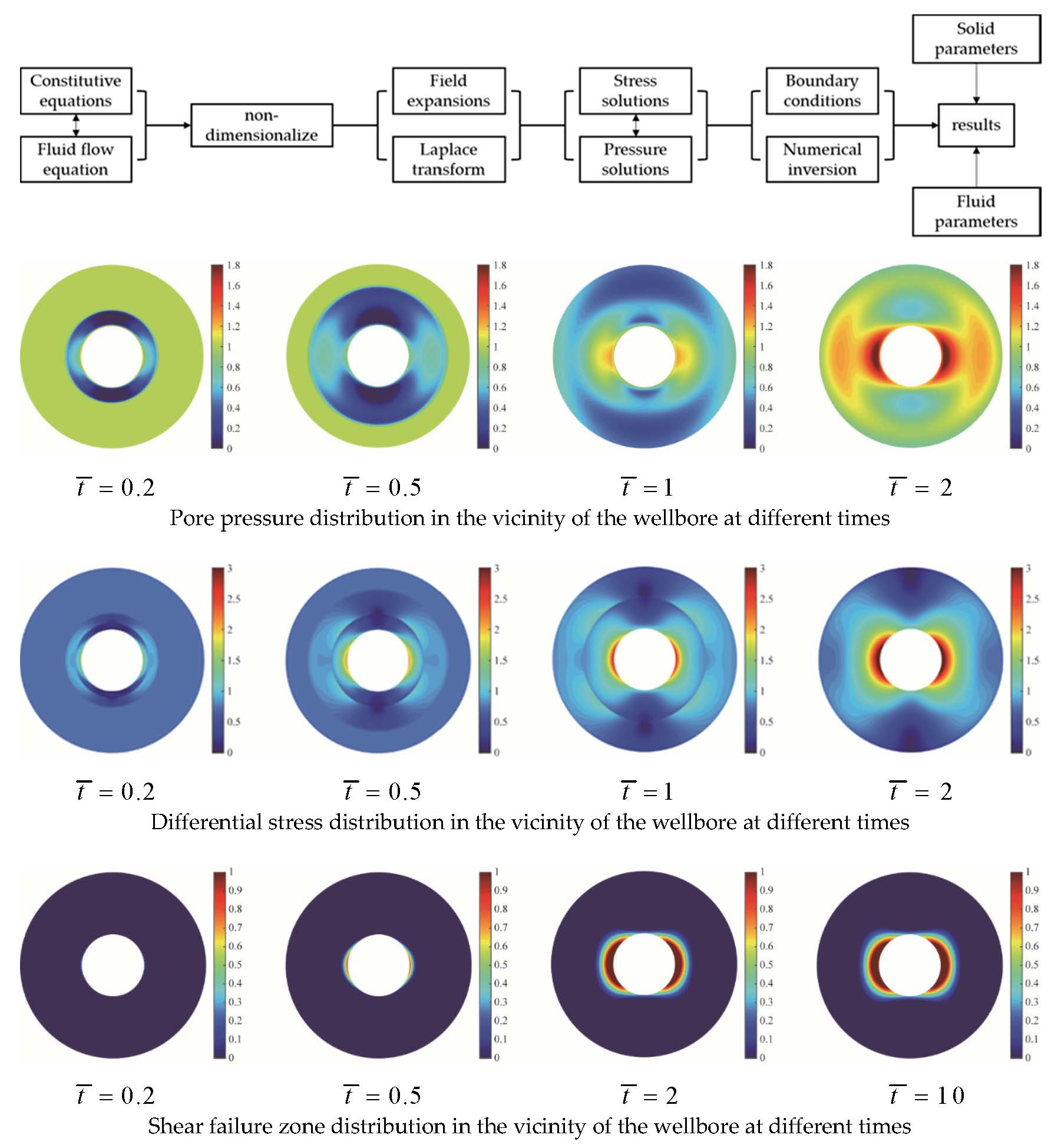
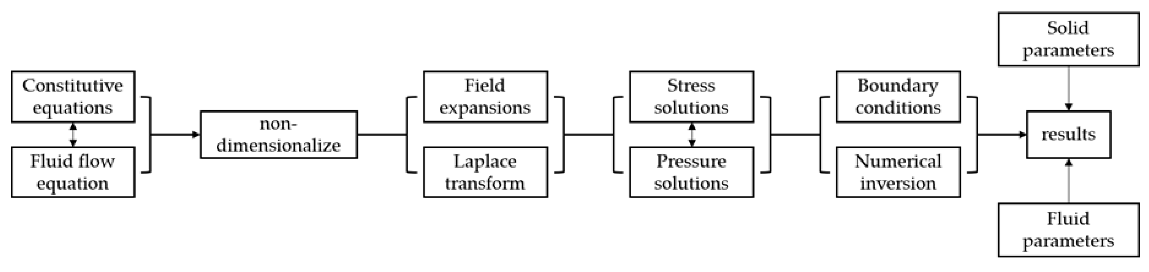
3. Solution Strategy

3.1. Field Expansions

As mentioned before, we consider a vertical wellbore drilled in a formation characterized by a non-hydrostatic horizontal in-situ stress field, as shown in Figure 1. The problem can be considered as an asymmetric plane strain problem in polar coordinates. The original stress and pressure in polar coordinates are:

$${\overline{\sigma }}_{rr}^0=-\left({\overline{P}}_0-{\overline{S}}_0\cos 2\theta \right)$$

(24)

$${\overline{\sigma }}_{\theta \theta }^0=-\left({\overline{P}}_0+{\overline{S}}_0\cos 2\theta \right)$$

(25)

$${\overline{\sigma }}_{r\theta }^0=-{\overline{S}}_0\sin 2\theta$$

(26)

$${\overline{p}}^0={\overline{p}}_0$$

(27)

where ${\overline{P}}_0$ and ${\overline{S}}_0$ are the far-field mean and deviatoric parts of the stresses; ${\overline{p}}_0$ is the unperturbed pore pressure; $\theta$ is the angle defined in Figure 1. The superscript 0 represents the original value. With the consideration of symmetry, as used in the poroelastic theory [28,29,30], the field expansions of the solutions should be sought to have the following form according to the far-field stresses:

$$\left\{e,{\overline{u}}_r,{\overline{\sigma }}_{rr},{\overline{\sigma }}_{\theta \theta },\overline{p}\right\}=\left\{e^{\left(0\right)},{\overline{u}}_r^{\left(0\right)},{\overline{\sigma }}_{rr}^{\left(0\right)},{\overline{\sigma }}_{\theta \theta }^{\left(0\right)},{\overline{p}}^{\left(0\right)}\right\}+\left\{e^{\left(2\right)},{\overline{u}}_r^{\left(2\right)},{\overline{\sigma }}_{rr}^{\left(2\right)},{\overline{\sigma }}_{\theta \theta }^{\left(2\right)},{\overline{p}}^{\left(2\right)}\right\}\cos 2\theta$$

(28)

$$\left\{{\overline{u}}_{\theta },{\overline{\sigma }}_{r\theta }\right\}=\left\{{\overline{u}}_{\theta }^{\left(2\right)},{\overline{\sigma }}_{r\theta }^{\left(2\right)}\right\}\sin 2\theta$$

(29)

where the superscript $\left(0\right)$ represents the axisymmetric mode solution, while $\left(2\right)$ represents the asymmetric mode solution resulting from the far-field deviatoric part of the stress.

3.2. Solutions in the Laplace Domain

The Laplace transform technique is used to solve the governing equations. By applying the Laplace transformation to Equation (19) and Equation (20), we obtain the transformed governing equations:

$$\left[\begin{array}{cc}1& -1\\ 0& 1\end{array}\right]\left\{\begin{array}{c}{\overline{\nabla }}_n^2{\tilde{e}}_n\\ {\overline{\nabla }}_n^2{\tilde{\overline{p}}}_n\end{array}\right\}=\left[\begin{array}{cc}{s}^2{\overline{\mathsf{\Phi }}}_1& s^2{\overline{\mathsf{\Phi }}}_2\\ s{\overline{\mathsf{\Omega }}}_1+s^2{\overline{\mathsf{\Phi }}}_3& s{\overline{\mathsf{\Omega }}}_2+s^2{\overline{\mathsf{\Phi }}}_4\end{array}\right]\left\{\begin{array}{c}{\tilde{e}}_n\\ {\tilde{\overline{p}}}_n\end{array}\right\}$$

(30)

In each mode $n(n=0,2)$, the transformed variables satisfy the dimensionless governing equations. Equation (30) can be decoupled and solved:

$${\tilde{e}}_n=A_n{K}_n\left({\beta }_1\overline{r}\right)+B_n{K}_n\left({\beta }_2\overline{r}\right)$$

(31)

$${\tilde{\overline{p}}}_n={\chi }_1{A}_n{K}_n\left({\beta }_1\overline{r}\right)+{\chi }_2{B}_n{K}_n\left({\beta }_2\overline{r}\right)$$

(32)

where:

$${\beta }_i=\frac{{\xi }_1\pm \sqrt{{\xi }_1^2-4{\xi }_2}}{2}$$

(33)

$${\chi }_i=\frac{{\beta }_i^2-s^2{\overline{\mathsf{\Phi }}}_1}{{\beta }_i^2+s^2{\overline{\mathsf{\Phi }}}_2}$$

(34)

$${\xi }_1=s\left({\overline{\mathsf{\Omega }}}_1+{\overline{\mathsf{\Omega }}}_2\right)+s^2\left({\overline{\mathsf{\Phi }}}_1+{\overline{\mathsf{\Phi }}}_3+{\overline{\mathsf{\Phi }}}_4\right)$$

(35)

$${\xi }_2=s^3\left({\overline{\mathsf{\Phi }}}_1{\overline{\mathsf{\Omega }}}_2+{\overline{\mathsf{\Phi }}}_1{\overline{\mathsf{\Phi }}}_{4}s-{\overline{\mathsf{\Phi }}}_2{\overline{\mathsf{\Omega }}}_1-{\overline{\mathsf{\Phi }}}_2{\overline{\mathsf{\Phi }}}_{3}s\right)$$

(36)

$A_n$ and $B_n$ are parameters depending only on $s$ and can be determined by boundary conditions. Combining Equations (5), (6) and (15) and performing non-dimensionalization and Laplace transformation result in the following coupled equations:

$${\overline{\nabla }}^2{\tilde{\overline{u}}}_{rn}-\frac{1}{{\overline{r}}^2}\left(2n{\tilde{\overline{u}}}_{\theta n}+{\tilde{\overline{u}}}_{rn}\right)+{\overline{\mathsf{\Psi }}}_1\frac{\partial {\tilde{e}}_n}{\partial \overline{r}}+{\overline{\mathsf{\Psi }}}_2\frac{\partial {\tilde{\overline{p}}}_n}{\partial \overline{r}}={\overline{\mathsf{\Psi }}}_3^2{\tilde{\overline{u}}}_{rn}$$

(37)

$$-{\overline{\nabla }}^2{\tilde{\overline{u}}}_{\theta n}+\frac{1}{{\overline{r}}^2}\left({\tilde{\overline{u}}}_{\theta n}+2n{\tilde{\overline{u}}}_{rn}\right)+{\overline{\mathsf{\Psi }}}_1\frac{n{\tilde{e}}_n}{\overline{r}}+{\overline{\mathsf{\Psi }}}_2\frac{n{\tilde{\overline{p}}}_n}{\overline{r}}=-{\overline{\mathsf{\Psi }}}_3^2{\tilde{\overline{u}}}_{\theta n}$$

(38)

where:

$${\overline{\mathsf{\Psi }}}_1=\frac{\lambda +\mu }{\mu },{\overline{\mathsf{\Psi }}}_2=\frac{\left(1-{\overline{\mathsf{\Phi }}}_1\right)\left(\lambda +2\mu \right)s^2}{\mu \alpha \eta }-\frac{\lambda +2\mu }{\mu },{\overline{\mathsf{\Psi }}}_3^2=\frac{\lambda +2\mu }{\mu }{s}^2-\frac{{\left(1-{\overline{\mathsf{\Phi }}}_1\right)}^2\left(\lambda +2\mu \right)s^4}{\mu \alpha \eta }$$

(39)

$$\eta =\frac{{\overline{\mathsf{\Omega }}}_{1}s}{\alpha }+\frac{{\overline{\mathsf{\Omega }}}_1{\overline{\mathsf{\Phi }}}_4{s}^2}{\alpha {\overline{\mathsf{\Omega }}}_2}$$

(40)

A technique is used to eliminate the displacement curl that the displacement components can be mapped into the following functions [29]:

$${\mathsf{\Pi }}_n={\tilde{\overline{u}}}_{rn}-{\tilde{\overline{u}}}_{\theta n}$$

(41)

$${\mathsf{\Lambda }}_n={\tilde{\overline{u}}}_{rn}+{\tilde{\overline{u}}}_{\theta n}$$

(42)

After some algebraic manipulations involving Equations (31), (32), (37) and (38), we can obtain the governing equations of the modified displacement functions ${\mathsf{\Pi }}_n$ and ${\mathsf{\Lambda }}_n$:

$$\left({\overline{\nabla }}_{n-1}^2-{\overline{\mathsf{\Psi }}}_3^2\right){\mathsf{\Pi }}_n={\Delta }_1{\beta }_1{A}_n{K}_{n-1}\left({\beta }_1\overline{r}\right)+{\Delta }_2{\beta }_2{B}_n{K}_{n-1}\left({\beta }_2\overline{r}\right)$$

(43)

$$\left({\overline{\nabla }}_{n+1}^2-{\overline{\mathsf{\Psi }}}_3^2\right){\mathsf{\Lambda }}_n={\Delta }_1{\beta }_1{A}_n{K}_{n+1}\left({\beta }_1\overline{r}\right)+{\Delta }_2{\beta }_2{B}_n{K}_{n+1}\left({\beta }_2\overline{r}\right)$$

(44)

where:

$${\Delta }_i={\overline{\mathsf{\Psi }}}_1+{\overline{\mathsf{\Psi }}}_2{\chi }_i=-\frac{{\beta }_i^2-{\overline{\mathsf{\Psi }}}_3^2}{{\beta }_i^2}$$

(45)

Through the solution of ordinary differential equations, Equations (43) and (44), which involves some manipulations, we can obtain the general expressions for the displacement components in the Laplace transform domain, and the dynamic stress distribution finally yields:

$$\begin{array}{ll}{\tilde{\overline{\sigma }}}_{rr}^n& =A_n\left\{\frac{\overline{\lambda }}{2{\beta }_1\overline{r}}\left[K_{n-1}\left({\beta }_1\overline{r}\right)+K_{n+1}\left({\beta }_1\overline{r}\right)\right]+\frac{\overline{\lambda }{n}^2}{{\beta }_1^2{\overline{r}}^2}{K}_n\left({\beta }_1\overline{r}\right)+\left(1-{\chi }_1\right)K_n\left({\beta }_1\overline{r}\right)\right\}\\ & +B_n\left\{\frac{\overline{\lambda }}{2{\beta }_2\overline{r}}\left[K_{n-1}\left({\beta }_2\overline{r}\right)+K_{n+1}\left({\beta }_2\overline{r}\right)\right]+\frac{\overline{\lambda }{n}^2}{{\beta }_2^2{\overline{r}}^2}{K}_n\left({\beta }_2\overline{r}\right)+\left(1-{\chi }_2\right)K_n\left({\beta }_2\overline{r}\right)\right\}\\ & +C_n\left\{\frac{n\overline{\lambda }}{{\overline{r}}^2}{K}_n\left({\overline{\mathsf{\Psi }}}_3\overline{r}\right)+\frac{n{\overline{\mathsf{\Psi }}}_3\overline{\lambda }}{2\overline{r}}\left[K_{n-1}\left({\overline{\mathsf{\Psi }}}_3\overline{r}\right)+K_{n+1}\left({\overline{\mathsf{\Psi }}}_3\overline{r}\right)\right]\right\}\end{array}$$

(46)

$$\begin{array}{ll}{\tilde{\overline{\sigma }}}_{\theta \theta }^n& =A_n\left\{-\frac{\overline{\lambda }}{4}\left[K_{n-2}\left({\beta }_1\overline{r}\right)+2K_n\left({\beta }_1\overline{r}\right)+K_{n+2}\left({\beta }_1\overline{r}\right)\right]+\left(1-{\chi }_1\right)K_n\left({\beta }_1\overline{r}\right)\right\}\\ & +B_n\left\{-\frac{\overline{\lambda }}{4}\left[K_{n-2}\left({\beta }_2\overline{r}\right)+2K_n\left({\beta }_2\overline{r}\right)+K_{n+2}\left({\beta }_2\overline{r}\right)\right]+\left(1-{\chi }_2\right)K_n\left({\beta }_2\overline{r}\right)\right\}\\ & +C_n\left\{-\frac{n{\overline{\mathsf{\Psi }}}_3}{2\overline{r}}\left[K_{n-1}\left({\overline{\mathsf{\Psi }}}_3\overline{r}\right)+K_{n+1}\left({\overline{\mathsf{\Psi }}}_3\overline{r}\right)\right]-\frac{n\overline{\lambda }}{{\overline{r}}^2}{K}_n\left({\overline{\mathsf{\Psi }}}_3\overline{r}\right)\right\}\end{array}$$

(47)

$$\begin{array}{ll}{\tilde{\overline{\sigma }}}_{r\theta }^n& =A_n\left\{\frac{n\overline{\lambda }}{2{\beta }_1\overline{r}}\left[K_{n-1}\left({\beta }_1\overline{r}\right)+K_{n+1}\left({\beta }_1\overline{r}\right)\right]+\frac{\overline{\lambda }n}{{\beta }_1^2{\overline{r}}^2}{K}_n\left({\beta }_1\overline{r}\right)\right\}\\ & +B_n\left\{\frac{n\overline{\lambda }}{2{\beta }_2\overline{r}}\left[K_{n-1}\left({\beta }_2\overline{r}\right)+K_{n+1}\left({\beta }_2\overline{r}\right)\right]+\frac{\overline{\lambda }n}{{\beta }_2^2{\overline{r}}^2}{K}_n\left({\beta }_2\overline{r}\right)\right\}\\ & +C_n\left\{\begin{array}{l}\frac{n^2\overline{\lambda }}{2{\overline{r}}^2}{K}_n\left({\overline{\mathsf{\Psi }}}_3\overline{r}\right)+\frac{{\overline{\mathsf{\Psi }}}_3\overline{\lambda }}{4\overline{r}}\left[K_{n-1}\left({\overline{\mathsf{\Psi }}}_3\overline{r}\right)+K_{n+1}\left({\overline{\mathsf{\Psi }}}_3\overline{r}\right)\right]\\ +\frac{{\overline{\mathsf{\Psi }}}_3^2\overline{\lambda }}{8}\left[K_{n-2}\left({\overline{\mathsf{\Psi }}}_3\overline{r}\right)+2K_n\left({\overline{\mathsf{\Psi }}}_3\overline{r}\right)+K_{n+2}\left({\overline{\mathsf{\Psi }}}_3\overline{r}\right)\right]\end{array}\right\}\end{array}$$

(48)

3.3. Boundary Conditions

The analytical solutions presented above, together with the appropriate boundary conditions at the wellbore, can be used to analyze the transient failure responses. We consider the drilling of a vertical borehole by a bit generates periodic loads at the bottom hole (the Sinusoidal and Cosine loads are considered in this paper). In the axisymmetric mode $(n=0)$, $C_0=0$ and the remaining two constants $A_0$ and $B_0$ can be computed by the radial stress and pore pressure boundary conditions. If we assume a Sinusoidal oscillation of the bottom-hole pressure around a constant value ${\overline{p}}_w$ with an amplitude $2L$ and an angular frequency $\omega$ (as shown in Figure 2), then the stress and pore pressure boundary conditions in the axisymmetric mode $(n=0)$ can be written in the Laplace domain:

$${\tilde{\overline{\sigma }}}_{rr}^0\left(1,s\right)=\frac{1}{s}\left({\overline{P}}_0-{\overline{p}}_w\right)-\frac{\omega L}{s^2+{\omega }^2}$$

(49)

$${\tilde{\overline{p}}}_0\left(1,s\right)=\frac{1}{s}\left({\overline{p}}_w-{\overline{p}}_0\right)+\frac{\omega L}{s^2+{\omega }^2}$$

(50)

In the asymmetric mode $(n=2)$, the stress release at the wellbore results from the deviatoric parts of the far-field stress. After drilling, the rotational waves are coupled with compressional waves to propagate into the formation. The three constants $A_2$, $B_2$, $C_2$ should be determined by the trigonometric part of radial stress, hoop stress and pore pressure applied at the wellbore surface after removing the far-field values, which can be expressed in the Laplace domain as:

$${\tilde{\overline{\sigma }}}_{rr}^2\left(1,s\right)=-\frac{{\overline{S}}_0}{s}$$

(51)

$${\tilde{\overline{\sigma }}}_{r\theta }^2\left(1,s\right)=\frac{{\overline{S}}_0}{s}$$

(52)

$${\tilde{\overline{p}}}^2\left(1,s\right)=0$$

(53)

These boundary conditions must be used for closed solutions.

3.4. Numerical Method

The solutions presented in the Laplace domain should be carefully inverted to the real time domain. Since the solutions reflect the wave propagation phenomenon, the method of Crump is employed which uses a truncated Fourier series to approximate the complex inversion integral. This method serves a more accurate algorithm particularly suitable for transient and highly oscillatory problems [31]. The method of Crump approximates the inversion integral using the following equation [25]:

$$f\left(t\right)=\frac{e^{at}}{t}\left\{\frac{1}{2}F\left(a\right)+\mathrm{Re}{\displaystyle \sum _{k=1}^{n}F\left(a+\frac{k\pi }{t}i\right){\left(-1\right)}^k}\right\}$$

(54)

where $i=\sqrt{-1}$, and the parameters $a$ and $n$ must be optimized, and generally we can set $at=4.5$ and $n=100$ to have a good accuracy [25]. Figure 3 shows the modeling methodology with user-defined input parameters for a better understanding of the method proposed in this work.

4. Stress Distribution and Failure Responses

In all the computations and plots, the stress components and pressure are scaled by the original pore pressure value. The values of the used dimensional parameters are listed in

Table 1. Parameter sets used in the calculation.

Parameter	Value	Parameter	Value
Shear modulus $\mu$ [GPa]	10	Lame constant $\lambda$ [GPa]	7
Biot coefficient $\alpha$	0.6	Biot modulus $M$ [GPa]	10
Pore fluid density ${\rho }_f$ [kg·m−3]	300	Rock density $\rho$ [kg·m−3]	2800
Rock permeability $\kappa$ [mD]	0.8	Pore fluid viscosity $\tau$ [Pa·s]	3 × 10−5
Tortuosity factor $a$	1.6	Rock porosity $\varphi$	0.06
Maximum principal stress ${\sigma }_H$ [MPa]	130	Minimum principal stress ${\sigma }_h$ [MPa]	100
Initial pore pressure $p_0$ [MPa]	50	Wellbore radius $r_w$ [m]	0.1

. These values are selected from a gas well in Keshen block in Tarim oil field.

We assume a Sinusoidal oscillation of the bottom-hole pressure that holds:

$${\overline{p}}_h={\overline{p}}_w+L\sin \left(\omega \overline{t}\right)$$

(55)

where the dimensional bottom-hole pressure is 50 MPa and $L=0.2{\overline{p}}_w$, $\omega =10$.

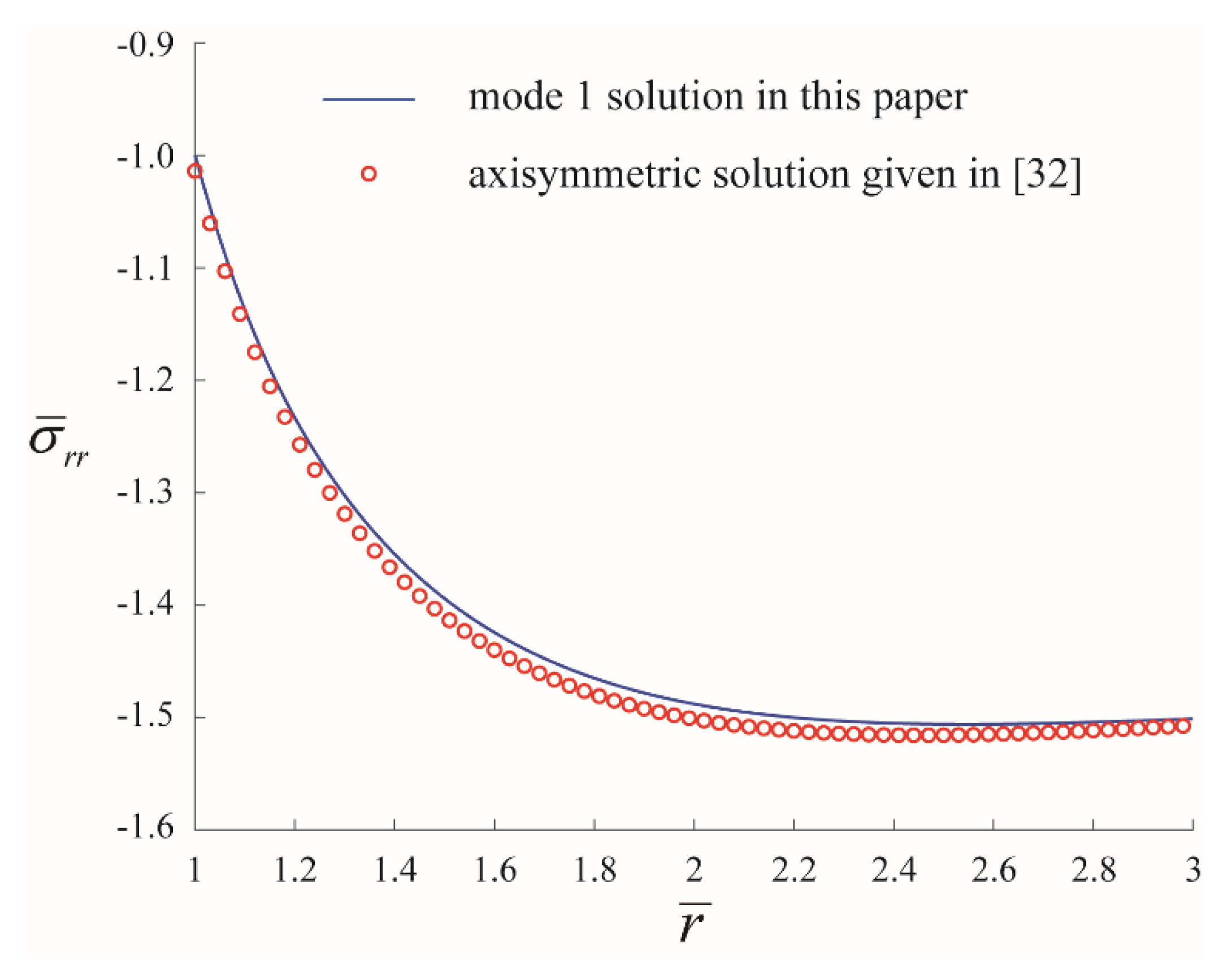
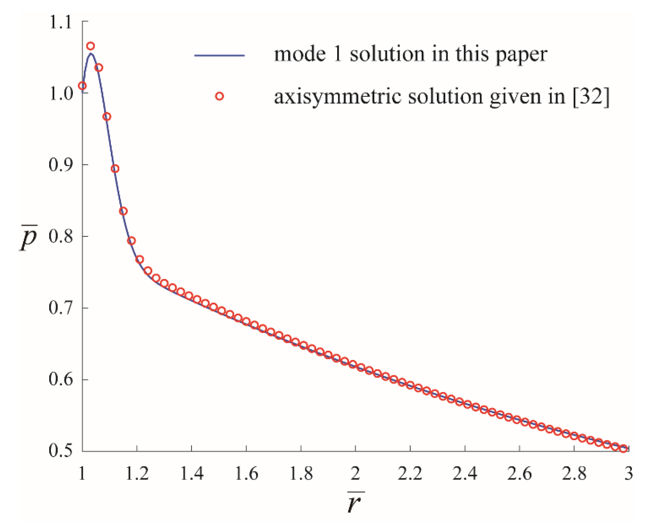
4.1. Model Verification

Since the existing models and poroelastodynamic solutions in the literature cannot be directly used for our problem, we first considered a simplified case where the bottom-hole pressure is constant and the two principal far-field stresses are the same, and thus, the problem becomes axisymmetric. Senjuntichai and Rajapakse [32] gave the axisymmetric solutions under constant fluid pressure that can be used in this simplified case. In our model, we considered the complex drilling conditions involving differential stress and periodic loads and used a different approach to solve the problem. The final solution is the superposition of an axisymmetric mode $(n=0)$ and an asymmetric mode $(n=2)$, and the two modes have the same form of the solution. To verify our solution, we compared the axisymmetric mode $(n=0)$ with the solution given by Senjuntichai and Rajapakse [32] using the input parameters defined in Table 1. The results are shown in Figure 4 and Figure 5 for the pressure and radial stress, respectively, which demonstrates that the axisymmetric mode solution obtained in this paper agrees well with the published solution [32] when the pressure is prescribed at the wellbore surface, although the solution strategy is different. This comparison shows the validity and the robustness of the model and solution.

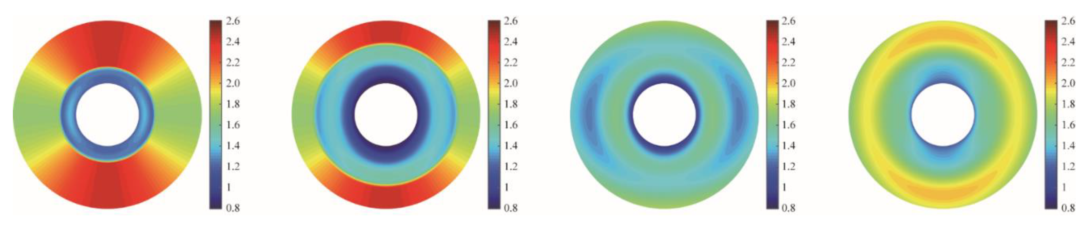
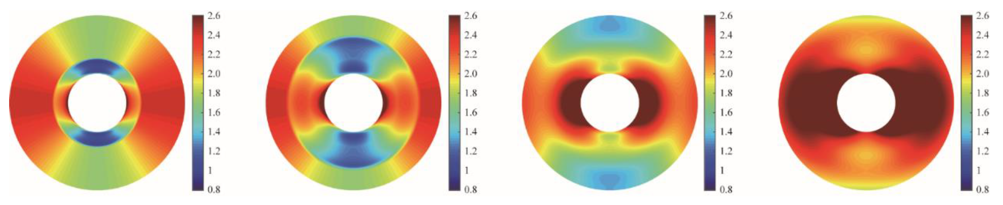
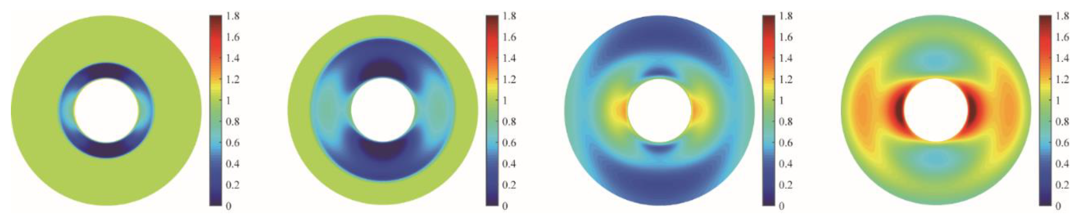
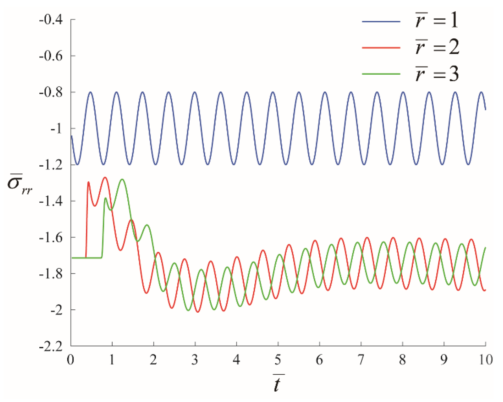
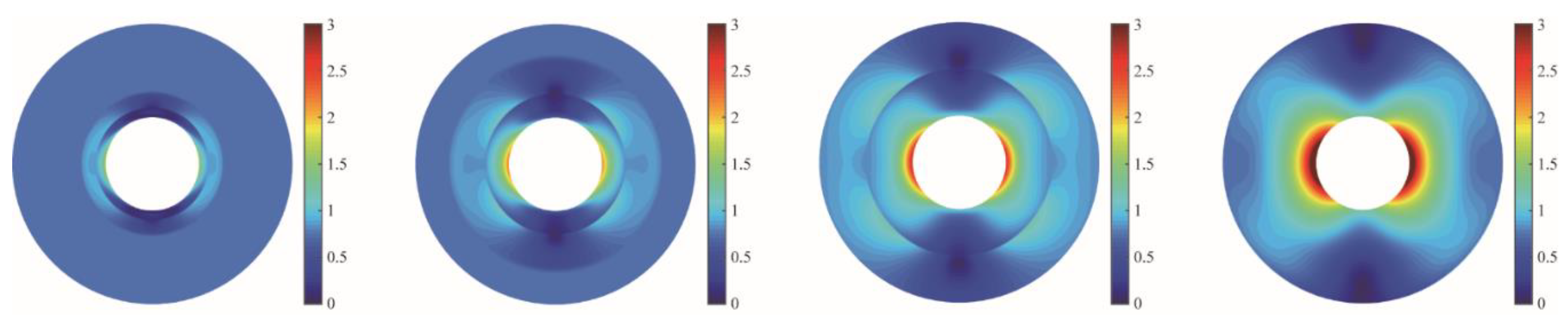
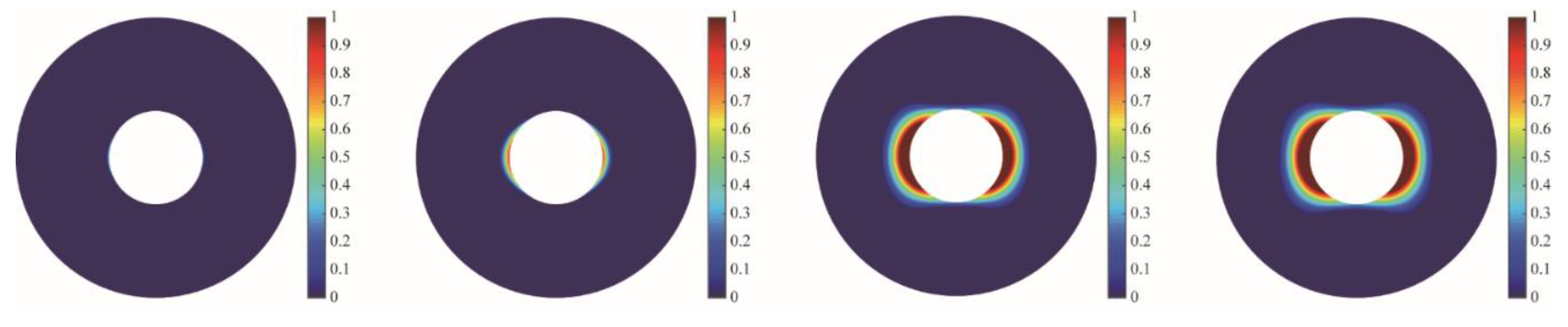
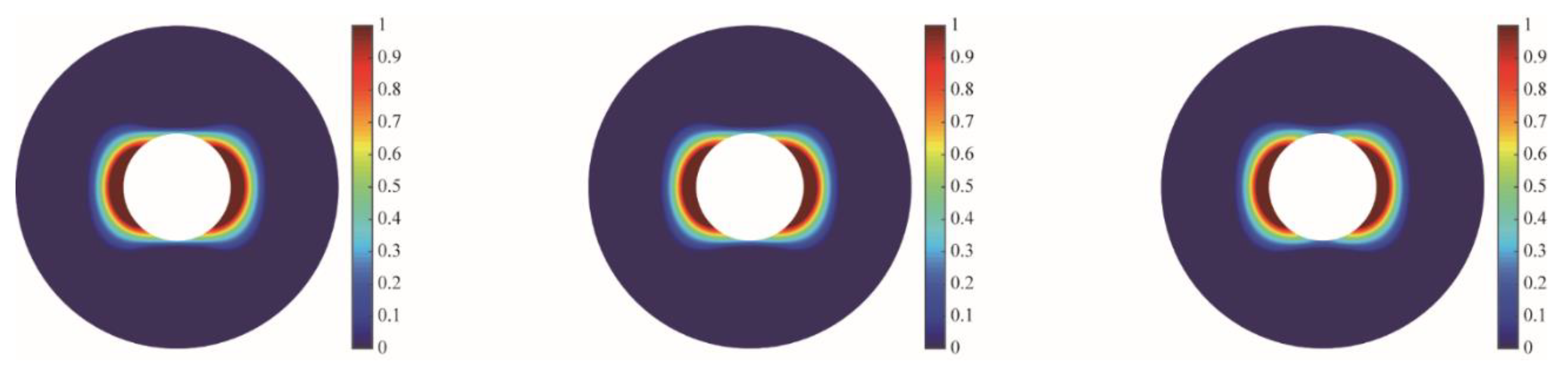
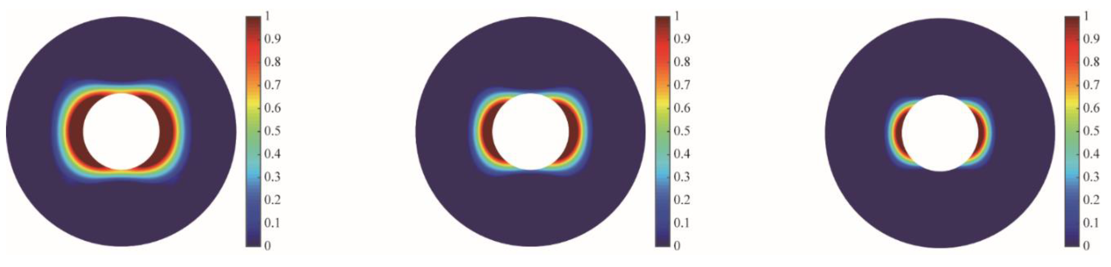
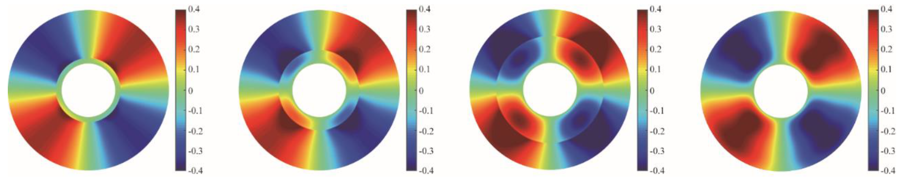
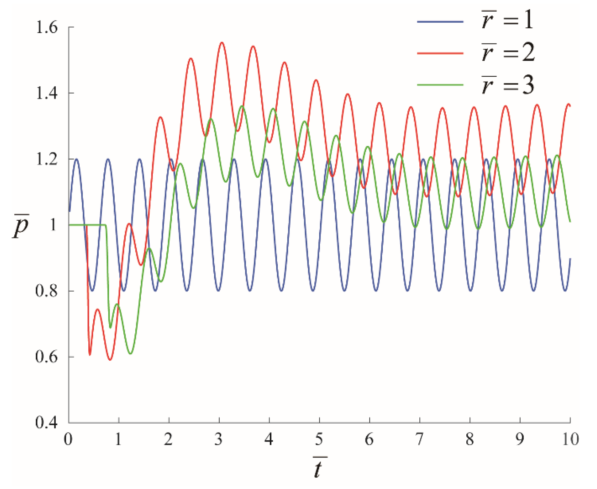
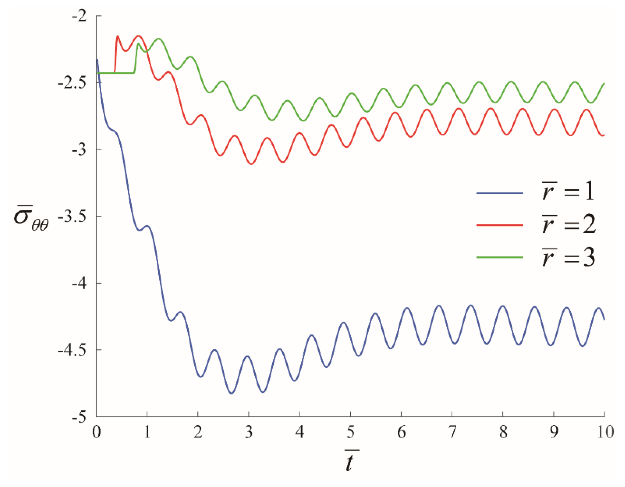
4.2. Dynamic Distributions of Stress Components and Pressure

We first examined the profiles of stress components with the two-dimensional isobaric plots for the solutions. Figure 6, Figure 7 and Figure 8 show the dynamic distribution of stress components in the vicinity of the wellbore. The values in all the figures in this paper are dimensionless. It can be seen from the results that the stress components are all characterized by wave-propagation properties during the drilling process, and the stress perturbation applied at the wellbore surface propagates into the formation. At an early time after drilling ($\overline{t}=0.2$ and $\overline{t}=0.5$ in Figure 6, Figure 7 and Figure 8), a disturbance zone is observed near the wellbore and expands as time increases. The stress components appear to fluctuate in the disturbance zone. The stress outside the disturbance zone keeps the original state and the disturbance boundary propagates into the formation. The propagation velocity of the disturbance boundary equals the propagation velocity of the stress wave. It can be clearly seen from the plots that the wave velocities of radial and hoop stress are larger than that of the shear stress. Figure 9 shows the dynamic pore pressure distribution in the vicinity of the wellbore, which also exhibits fluctuations in the disturbance zone. Due to the sudden release of stress at the wellbore surface, the pore pressure near the wellbore decreases significantly at the beginning of drilling, even to a negative value. Then, due to the existence of the differential stress, the pore pressure increases in the direction of the minimum principal stress and gradually reaches a much higher value compared to the initial pore pressure.

The maximum shear stress occurs in the direction of the minimum principal stress, and hence, shear failure at the wellbore surface initiates in the direction of the minimum principal stress [5]. In order to further analyze the dynamic evolution of stress and pore pressure in the formation, we selected three locations along the direction of minimum principal stress to analyze the time variation of the stress and pressure. The coordinates of the selected locations are $\left(\overline{r},\theta \right)=\left(1,0\right)$, $\left(2,0\right)$, $\left(3,0\right)$, respectively. Figure 10 shows the pressure fluctuation at the selected locations. The pressure at $\overline{r}=1$ is the given boundary condition that is a sinusoidal wave. Inside the wellbore ($\overline{r}=2$ and $\overline{r}=3$), the pore pressure decreases at the beginning and then increases to a peak, and finally approaches stable fluctuation. It is interesting to find the fluctuation amplitude decreases as distance increases. The pore pressure reaches its peak at a certain time and location, while the conventional poroelastic theory always fails to discover this phenomenon due to the lack of consideration of solid-fluid acceleration. Figure 11 shows the variation of radial stress with time at selected locations. The model in this paper assumes compression as negative, thus, the computed stresses are all negative. The radial stress at the wellbore surface equals the given pressure boundary condition. When the stress wave propagates to a certain location, the radial stress increases from the initial value at the beginning and then decreases, and finally approaches to stable fluctuation. Figure 12 shows the hoop stress fluctuation at the selected locations. Because the hoop stress is not given at the wellbore surface and the radial stress is suddenly released, the hoop compressive stress at the wellbore surface increases rapidly after drilling. The magnitudes of radial stress as well as hoop stress decrease as distance increases.

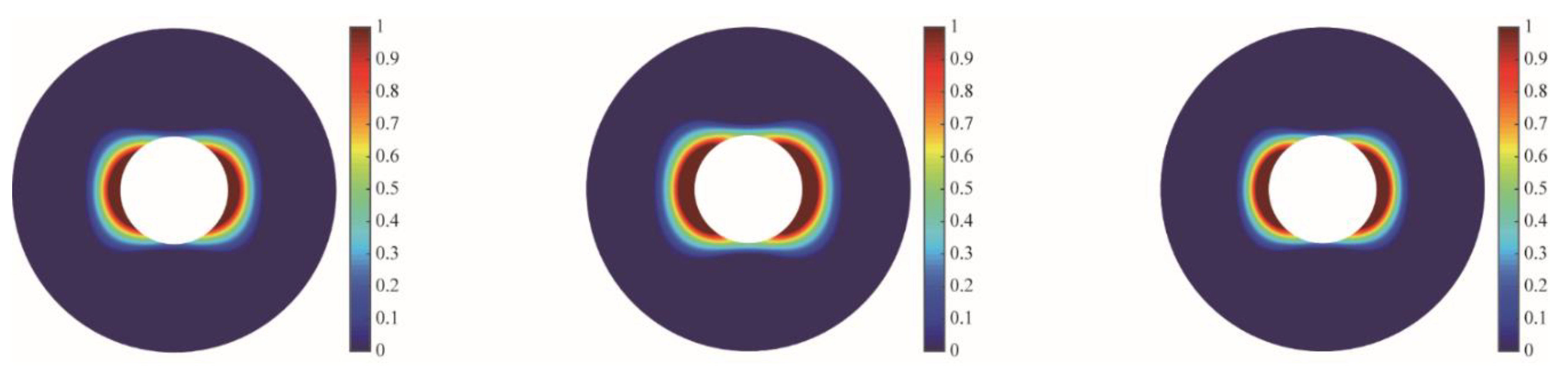
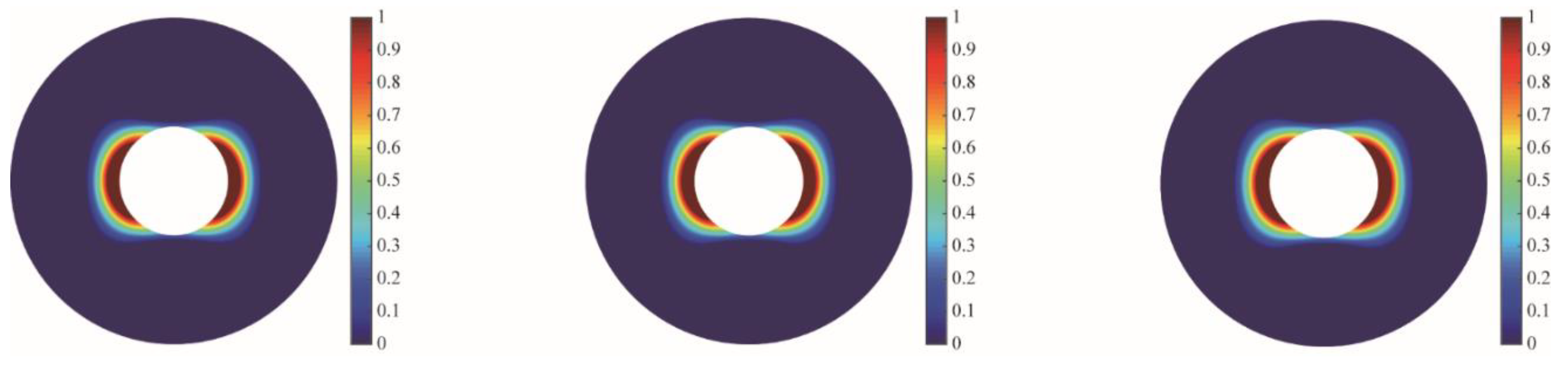
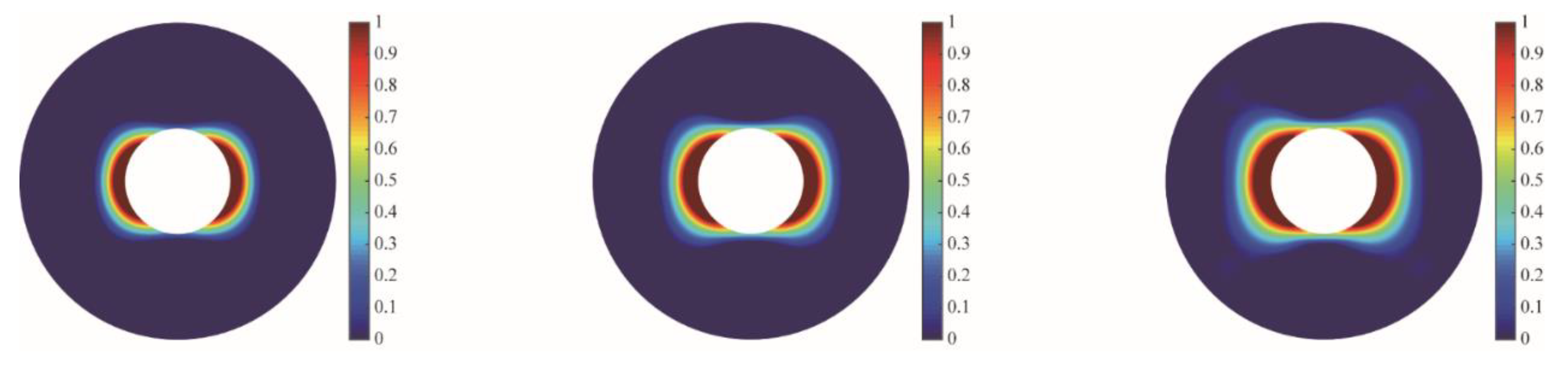
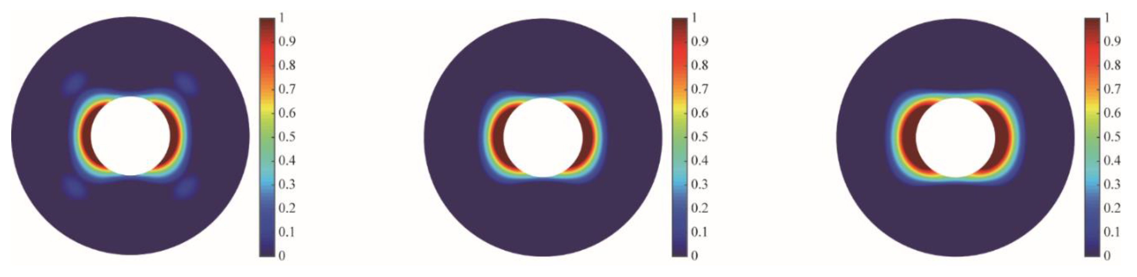
4.3. Failure Responses

We consider shear failure mode with the Mohr Coulomb criteria in this section to analyze the transient failure response. The failure criteria can be written as [28]:

$$F=\frac{\left|-\tan \phi \left({\sigma }_1+{\sigma }_3\right)+2C_t\right|}{\sqrt{{\tan }^2\phi +1}}-{\sigma }_3+{\sigma }_1\le 0$$

(56)

where $\phi$ is the internal friction angle and $C_t$ s the cohesion; ${\sigma }_1$ and ${\sigma }_3$ are the maximum and minimum principal stresses, respectively. We assume $\phi =20^{\circ }$ and $C_t=10 \mathrm{MPa}$. We first examine the dynamic profiles of the differential stress, i.e., ${\sigma }_1-{\sigma }_3$ at different times, and the results are shown in Figure 13. The differential stress at the wellbore surface is small at the beginning of drilling, and becomes larger in the direction of minimum principal stress as time increases, which results in a high-risk zone of shear failure. Figure 14 shows the variation of the differential stress with time at three selected locations in the direction of minimum principal stress and the coordinates are $\left(\overline{r},\theta \right)=\left(1,0\right)$, $\left(1.2,0\right)$, $\left(1.5,0\right)$. The differential stress also exhibits fluctuation characteristic at selected locations. However, different from the stress components, the amplitude of the differential stress almost keeps the same as distance increases. It is in accordance with expectation that the differential stress decreases with distance; thus, the shear failure is most likely to occur at the wellbore surface. Figure 15 shows the dynamic shear failure zone distribution in the vicinity of the wellbore. The values in the figures of shear failure zone distribution correspond to $F$ in Equation (56). When $F$ is greater than 0, dynamic shear failure occurs, and a greater $F$ value means more severe shear failure. At the beginning ($\overline{t}=0.2$), the wellbore is stable. As time increases, the stress wave propagates into the formation, and a symmetrical failure zone appears in the direction of the minimum principal stress, and the area of the failure zone gradually increases. In the following subsections, the influences of poroelastic parameters, in-situ stress and periodic load parameters on the shear failure responses are analyzed in a detailed parametric study.

4.3.1. Effect of Poroelastic Parameters

We investigate the shear failure response under various sets of poroelastic parameters, while keeping the rest at their baseline values: (i) the Lamé constant $\lambda$; (ii) the Biot coefficient $\alpha$; (iii) the Biot modulus $M$; (iv) the rock permeability $\kappa$. For a completely dry porous medium $M=0$, whereas for a material with incompressible constituents we have $M\to \infty$ and $\alpha \to 1$. The shear failure modes in response to different values of poroelastic parameters are plotted in Figure 16, Figure 17, Figure 18 and Figure 19, and each figure corresponds to variation in one of the four sets of parameters (i)–(iv). Among the four poroelastic parameters, the Lamé constant $\lambda$ has the slightest effect on the area of failure zone. A larger value of $\alpha$ or $M$ slightly enlarges the area of failure zone in the direction of the minimum principal stress. It is interesting to observe that a small value of $M$ (for example a gas reservoir) can cause a slight failure along the diagonal direction, which is isolated near the wellbore. A higher permeability $\kappa$ enables a higher speed of pressure diffusion so that it will shrink the failure area in the direction of the minimum principal stress and the wellbore becomes more stable.

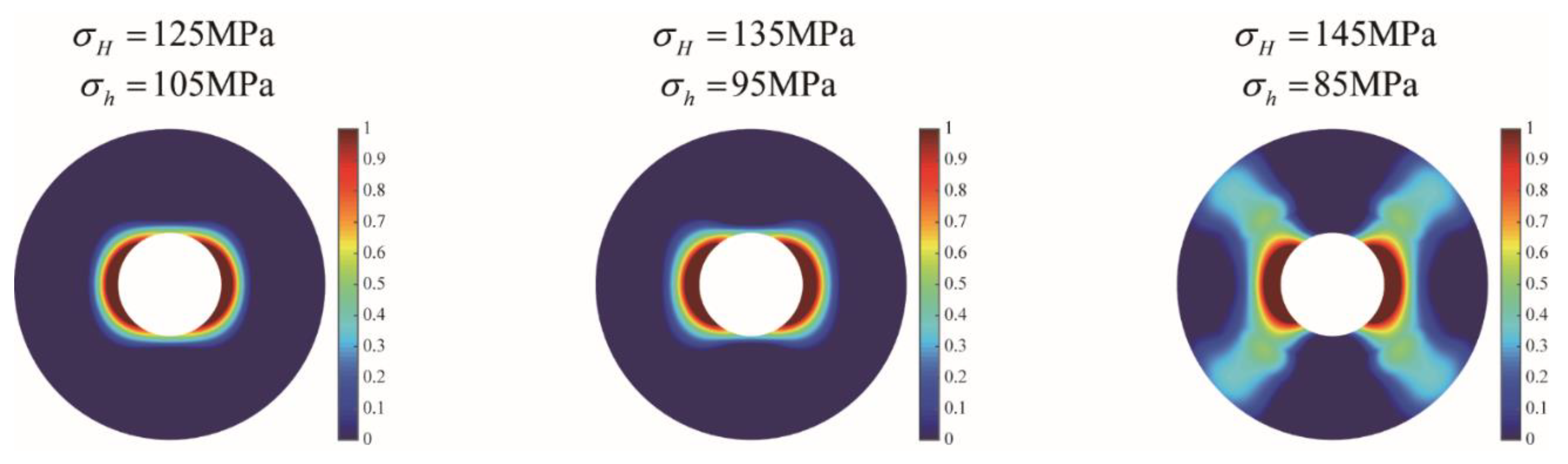
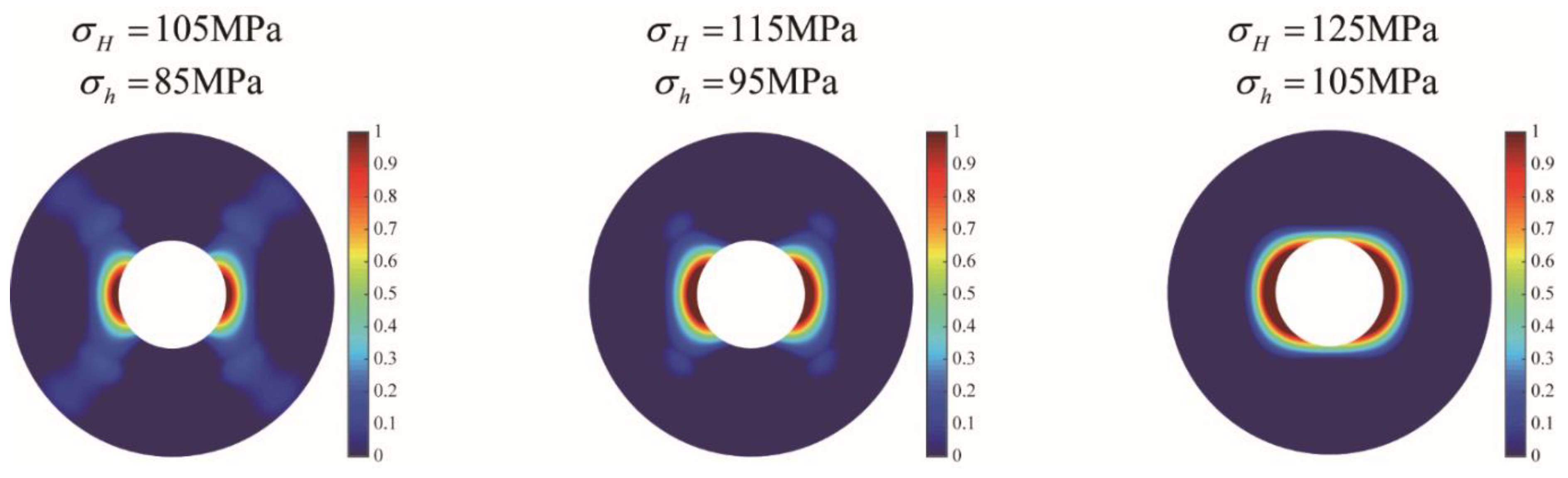
4.3.2. Effect of In-Situ Stress

In this subsection, we compute the shear failure responses under different in-situ stress states. Figure 20 shows the failure zone distribution in the vicinity of the wellbore with different deviatoric part of the stress while the mean part of the stress keeps the same. It can be seen from the plot that a larger differential stress results in a much more severe failure around the wellbore, especially in the diagonal direction. Figure 21 shows the failure zone distribution with different mean part of the stress while the deviatoric part of the stress keeps the same. It is interesting to find that a higher stress state with the same differential value results in a more severe failure response in the direction of the minimum principal stress; however, a smaller stress state can cause a slight failure along the diagonal direction, which is connected with the wellbore and greatly increases the area of the shear failure zone. Generally, a larger mean value of the original principal stress always indicates a deeper reservoir. We can conclude that a more severe wellbore instability occurs to a shallow reservoir compared to a deep reservoir, when the differential stress is the same.

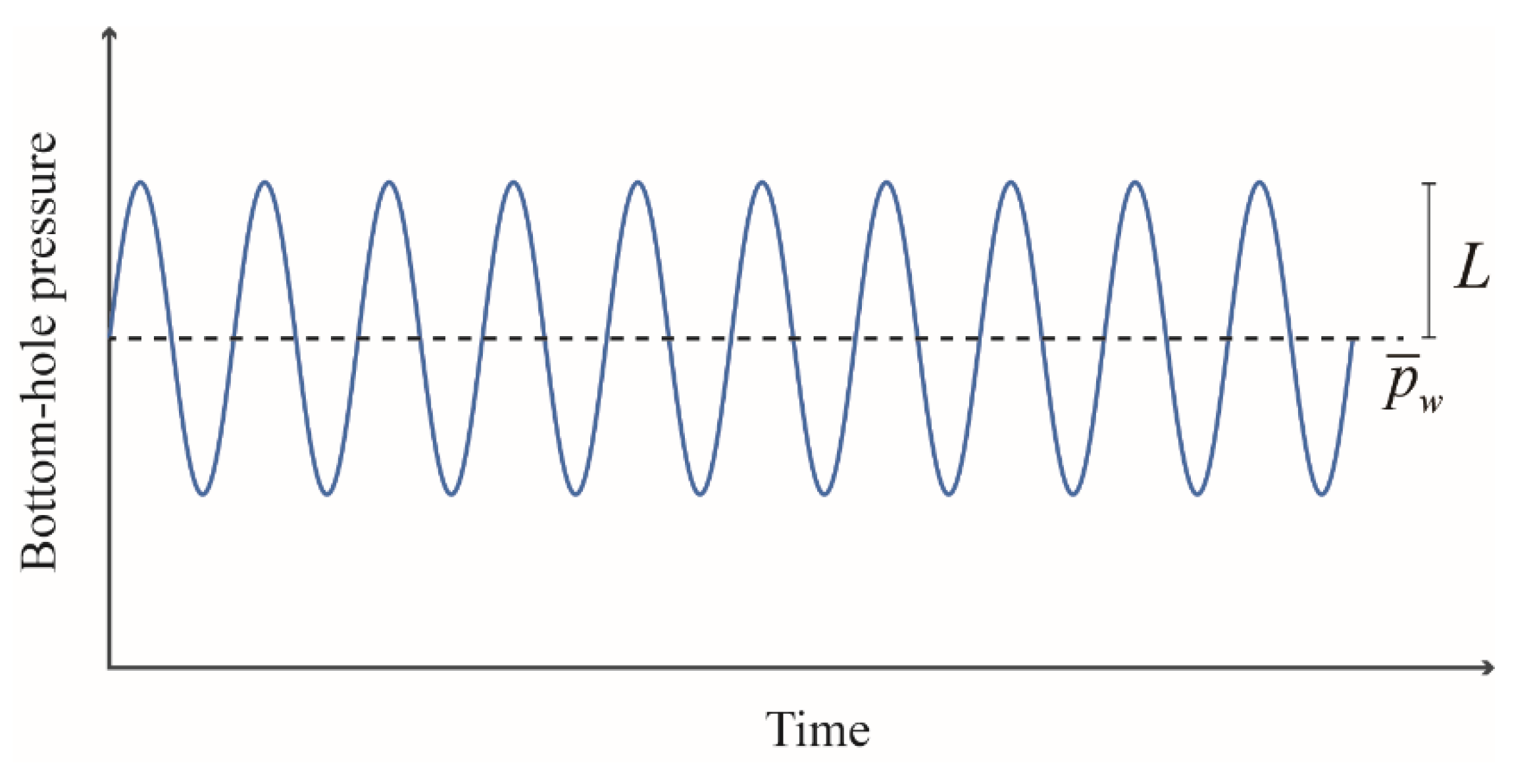
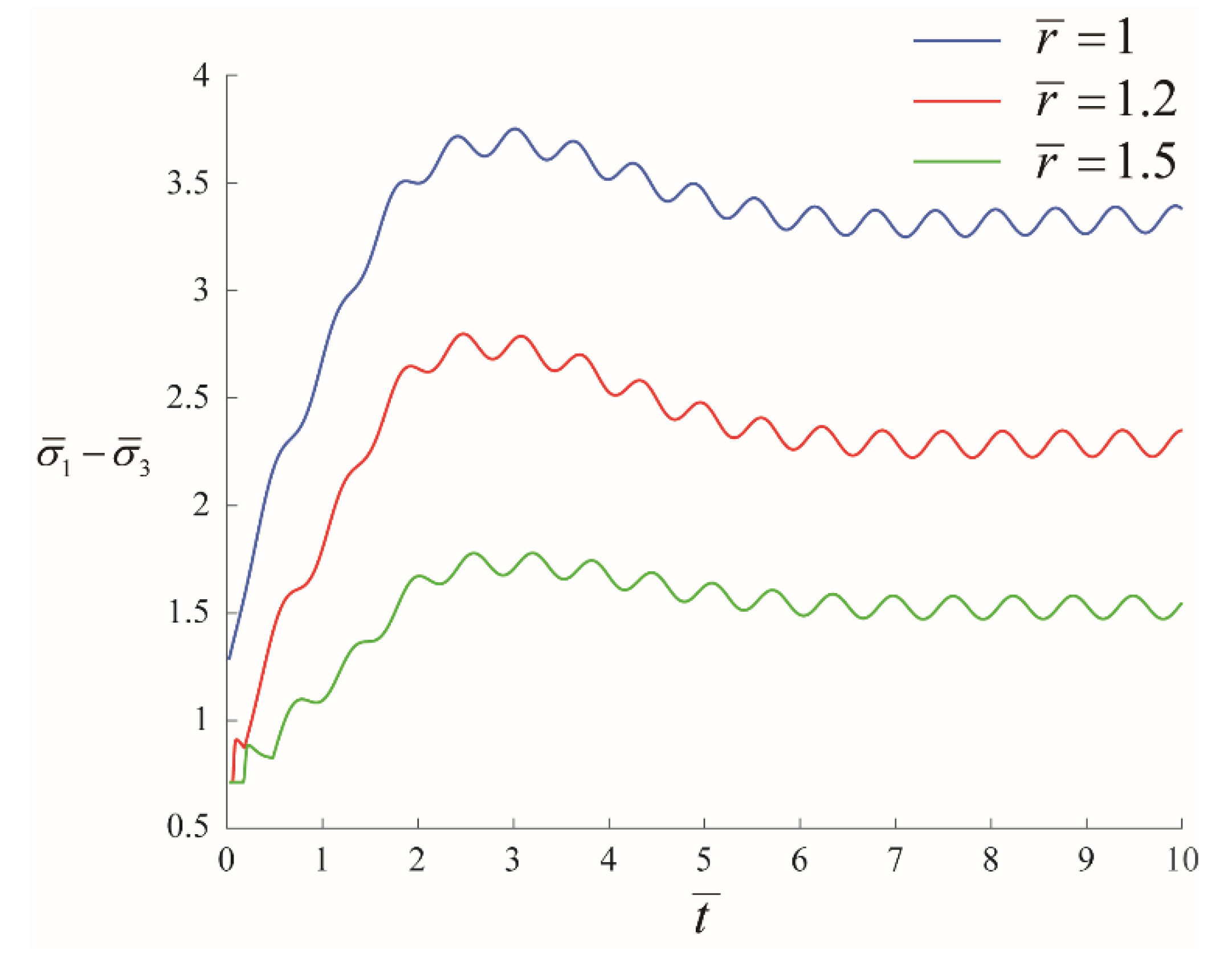
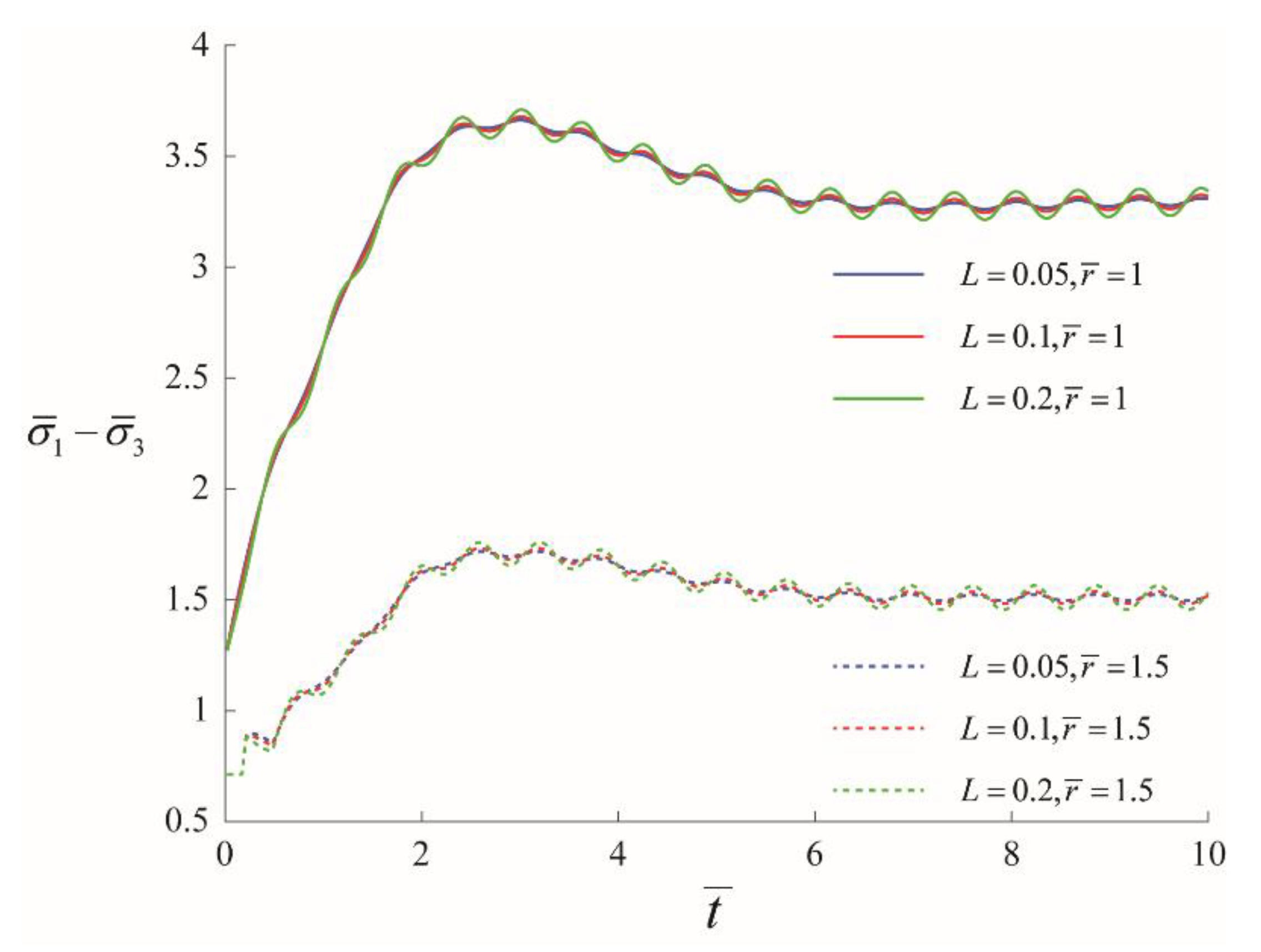
4.3.3. Effect of Periodic Loads

In this subsection, we analyze the effect of the parameter value of the given periodic load on the failure responses. We assume the bottom-hole pressure is periodically fluctuating, which can be caused by trips or bit vibration during drilling. The load is applied at the wellbore surface and can be mathematically described by a simple Sinusoidal function as shown in Equation (55). We considered three parameters: the mean value of the load ${\overline{p}}_w$, the angular frequency of the Sinusoidal load $\omega$ and the amplitude of the Sinusoidal load $L$. The load is non-dimensionalized by the initial pore pressure $p_0$. We first considered three cases: (i) ${\overline{p}}_w=0.9<1$, corresponding to an underbalanced drilling; (ii) ${\overline{p}}_w=1$, corresponding to a balanced drilling; (iii) ${\overline{p}}_w=1.1>1$, corresponding to an overbalanced drilling. Figure 22 shows the shear failure responses under the three conditions. Unsurprisingly, increasing the bottom-hole pressure helps maintain the wellbore stability. We then investigate the effect of the frequency of the periodic load on the failure response, and the results are shown in Figure 23. It is noteworthy that the failure is more severe at a certain value of the load frequency, and the area of the failure zone reaches a peak when $\omega =10$. The effect of amplitude of the Sinusoidal load is also examined, which is found to be negligible on the shear failure response, as shown in Figure 24. For further investigation, we calculate the differential stress at two selected locations in the direction of minimum principal stress, and the results are shown in Figure 25. The amplitude of the differential stress is found to be much smaller than the load amplitude, indicating that subtraction of the principal stress reduces the wave amplitude and decreases the risk of wellbore instability due to wave propagation.

Based on the results of the parametric study, we found that the in-situ stress, especially the differential stress, is the most critical parameter for wellbore stability. Moreover, the Biot coefficient $\alpha$, Biot modulus $M$, permeability $\kappa$, bottom-hole pressure $p_w$ and the frequency of the Sinusoidal load $\omega$ also impact the area of shear failure zone. Meanwhile, the Lamé constant $\lambda$ and the amplitude of the Sinusoidal load $2L$ have the slightest effect on the shear failure response. Thus, their effect can be ignored in practical analysis of wellbore stability.

5. Conclusions

This paper presents a poroelastodynamic model that is based on Biot’s theory to study transient stress distribution and failure response of a wellbore subjected to periodic loading during drilling. In response to the periodic load perturbation at the wellbore surface, pressure and stress waves are created and propagate into the formation. The wave phenomenon is characterized by introducing solid-fluid acceleration term into the coupling mass conservation equation. The solutions are obtained in the Laplace domain through a new method and inverted numerically to the real time domain using a reliable numerical scheme. The results show that a disturbance zone is created after drilling. Inside the disturbance zone, pressure and stress waves propagate; outside the disturbance zone, the pressure and stress keep the original state. The disturbance zone expands over time. When the stress waves propagate to a certain location, the pore pressure, radial and hoop stresses change rapidly at the beginning, and then reach a stable fluctuation. It was found that the wave velocities of radial stress, hoop stress and pressure are larger than that of the shear stress. It is noteworthy that pore pressure reaches its peak at a certain time and location, while the conventional poroelastic theory always fails to discover this phenomenon when a periodic load is applied on the wellbore due to the lack of consideration of solid-fluid acceleration.

Through the detailed parametric study on shear failure responses, we found that a smaller value of Biot coefficient $\alpha$ or Biot modulus $M$ can shrink the area of failure zone in the direction of the minimum principal stress and helps maintain wellbore stability. A higher permeability of a reservoir enables a higher speed of pressure diffusion so that it will also shrink the failure area and make the wellbore more stable. A larger differential stress of the original non-hydrostatic stress field results in a much more severe failure around the wellbore, especially in the diagonal direction. A larger mean value of the original non-hydrostatic stress field results in a more severe failure response in the direction of the minimum principal stress. However, a larger mean value of the original non-hydrostatic stress field helps to maintain stability along the diagonal direction. It is also noted that the wellbore instability is most severe at a certain value of the load frequency, which is dependent on the reservoir properties. It is suggested that the simulation should be performed prior to drilling to optimize the engineering parameters.

The model developed in this paper is 2D; however, 3D simulation is necessary for a directional well that is drilled in a deep reservoir. To solve 3D poroelastodynamics, Fourier transformation should be employed. One of the features in the deep reservoir is the extremely high temperature, which leads to the thermal dilation of the solid and fluid. Thus, the coupling of heat flux is an important future subject. In general, our model can be readily extended to 3D or thermal-poroelastodynamics.

References

1. Fjar, E.; Holt, R.M.; Raaen, A.M.; Risnes, R.; Horsrud, P. Petroleum Related Rock Mechanics; Elsevier: Amsterdam, The Netherlands, 2008. [Google Scholar]
2. Kirsch, C. Die theorie der elastizitat und die bedurfnisse der festigkeitslehre. Zeitschrift des Vereines Deutscher Ingenieure 1898, 42, 797–807. [Google Scholar]
3. Bradley, W.B. Failure of inclined boreholes. J. Energy Resour. Technol. 1979, 101, 232–239. [Google Scholar] [CrossRef]
4. Aadnoy, B.S.; Chenevert, M.E. Stability of highly inclined boreholes (includes associated papers 18596 and 18736). SPE Drill. Eng. 1987, 2, 364–374. [Google Scholar] [CrossRef]
5. Zoback, M.D. Reservoir Geomechanics; Cambridge University Press: Cambridge, UK, 2010. [Google Scholar]
6. Meng, M.; Zamanipour, Z.; Miska, S.; Yu, M.; Ozbayoglu, E.M. Dynamic stress distribution around the wellbore influenced by surge/swab pressure. J. Pet. Sci. Eng. 2019, 172, 1077–1091. [Google Scholar] [CrossRef]
7. Detournay, E.; Cheng, A.H.D. Poroelastic response of a borehole in a non-hydrostatic stress field. Int. J. Rock Mech. Min. Sci. Geomech. Abstr. 1988, 25, 171–182. [Google Scholar] [CrossRef]
8. Zamanipour, Z.; Miska, S.Z.; Hariharan, P.R. Effect of transient surge pressure on stress distribution around directional wellbores. In Proceedings of the IADC/SPE Drilling Conference and Exhibition, Fort Worth, TX, USA, 1–3 March 2016. [Google Scholar]
9. Zhang, F.; Kang, Y.; Wang, Z.; Miska, S.; Yu, M.; Zamanipour, Z. Transient coupling of swab/surge pressure and in-situ stress for wellbore-stability evaluation during tripping. SPE J. 2018, 23, 1019–1038. [Google Scholar] [CrossRef]
10. Meng, M.; Zamanipour, Z.; Miska, S.; Yu, M.; Ozbayoglu, E.M. Dynamic Wellbore Stability Analysis Under Tripping Operations. Rock Mech. Rock Eng. 2019, 1–21. [Google Scholar] [CrossRef]
11. Feng, Y.; Li, X.; Gray, K.E. An easy-to-implement numerical method for quantifying time-dependent mudcake effects on near-wellbore stresses. J. Pet. Sci. Eng. 2018, 164, 501–514. [Google Scholar] [CrossRef]
12. Chen, P.; Miska, S.Z.; Ren, R.; Yu, M.; Ozbayoglu, E.; Takach, N. Poroelastic modeling of cutting rock in pressurized condition. J. Pet. Sci. Eng. 2018, 169, 623–635. [Google Scholar] [CrossRef]
13. Biot, M.A. General theory of three-dimensional consolidation. J. Appl. Phys. 1941, 12, 155–164. [Google Scholar] [CrossRef]
14. Biot, M.A. Theory of propagation of elastic waves in a fluid-saturated porous solid, I: Low-frequency range. J. Acoust. Soc. Am. 1956, 28, 168–178. [Google Scholar] [CrossRef]
15. Biot, M.A. Theory of propagation of elastic waves in a fluid-saturated porous solid, II: Higher frequency range. J. Acoust. Soc. Am. 1956, 28, 179–191. [Google Scholar] [CrossRef]
16. Rasolofosaon, P.N.J. Importance of interface hydraulic condition on the generation of second bulk compressional wave in porous media. Appl. Phys. Lett. 1988, 52, 780–782. [Google Scholar] [CrossRef]
17. Kelder, O.; Smeulders, D.M.J. Propagation and damping of compressional waves in porous rocks: Theory and experiments. SEG Technical Program Expanded Abstracts 1995. Soc. Explor. Geophys. 1995, 675–678. [Google Scholar] [CrossRef]
18. Gurevich, B.; Kelder, O.; Smeulders, D.M.J. Validation of the slow compressional wave in porous media: Comparison of experiments and numerical simulations. Transp. Porous Media 1999, 36, 149–160. [Google Scholar] [CrossRef]
19. Schanz, M. Poroelastodynamics: Linear models, analytical solutions, and numerical methods. Appl. Mech. Rev. 2009, 62, 030803. [Google Scholar] [CrossRef]
20. Schanz, M.; Cheng, A.H.D. Transient wave propagation in a one-dimensional poroelastic column. Acta Mech. 2000, 145, 1–18. [Google Scholar] [CrossRef]
21. Xie, K.; Liu, G.; Shi, Z. Dynamic response of partially sealed circular tunnel in viscoelastic saturated soil. Soil Dyn. Earthq. Eng. 2004, 24, 1003–1011. [Google Scholar] [CrossRef]
22. Gao, M.; Wang, Y.; Gao, G.Y.; Yang, J. An analytical solution for the transient response of a cylindrical lined cavity in a poroelastic medium. Soil Dyn. Earthq. Eng. 2013, 46, 30–40. [Google Scholar] [CrossRef]
23. Liu, G.B.; Xie, K.H.; Yao, H.L. Scattering of elastic wave by a partially sealed cylindrical shell embedded in poroelastic medium. Int. J. Numer. Anal. Methods Geomech. 2005, 29, 1109–1126. [Google Scholar]
24. Hasheminejad, S.M.; Kazemirad, S. Dynamic response of an eccentrically lined circular tunnel in poroelastic soil under seismic excitation. Soil Dyn. Earthq. Eng. 2008, 28, 277–292. [Google Scholar] [CrossRef]
25. Xia, Y.; Jin, Y.; Chen, M.; Chen, K. Poroelastodynamic response of a borehole in a non-hydrostatic stress field. Int. J. Numer. Anal. Methods Geomech. 2017, 93, 82–93. [Google Scholar] [CrossRef]
26. Senjuntichai, T.; Keawsawasvong, S.; Plangmal, R. Three-dimensional dynamic response of multilayered poroelastic media. Mar. Georesour. Geotechnol. 2018, 37, 424–437. [Google Scholar] [CrossRef]
27. Keawsawasvong, S.; Senjuntichai, T. Poroelastodynamic fundamental solutions of transversely isotropic half-plane. Comput. Geotech. 2019, 106, 52–67. [Google Scholar] [CrossRef]
28. Xia, Y.; Jin, Y.; Wei, S.M.; Chen, M.; Zhang, Y.Y.; Lu, Y.H. Transient failure of a borehole excavated in a poroelastic continuum. Mech. Res. Commun. 2019. [Google Scholar] [CrossRef]
29. Mehrabian, A.; Abousleiman, Y.N. Generalized poroelastic wellbore problem. Int. J. Numer. Anal. Methods Geomech. 2013, 37, 2727–2754. [Google Scholar] [CrossRef]
30. Hasheminejad, S.M.; Hosseini, H. Dynamic stress concentration near a fluid-filled permeable borehole induced by general modal vibrations of an internal cylindrical radiator. Soil Dyn. Earthq. Eng. 2002, 22, 441–458. [Google Scholar] [CrossRef]
31. Hassanzadeh, H.; Pooladi-Darvish, M. Comparison of different numerical Laplace inversion methods for engineering applications. Appl. Math. Comput. 2007, 189, 1966–1981. [Google Scholar] [CrossRef]
32. Senjuntichai, T.; Rajapakse, R.K.N.D. Transient response of a circular cavity in a poroelastic medium. Int. J. Numer. Anal. Methods Geomech. 1993, 17, 357–383. [Google Scholar] [CrossRef]
Figure 1. Borehole in a non-hydrostatic stress field (from Xia et al. [25]), the load applied at the wellbore surface is periodic.
Energies 12 03486 g001
Figure 2. Example of a sinusoidal bottom-hole pressure.
Energies 12 03486 g002
Figure 3. Modeling methodology.
Energies 12 03486 g003
Figure 4. Comparison of pore pressure distribution using the simplified axisymmetric solution with constant bottom-hole pressure.
Energies 12 03486 g004
Figure 5. Comparison of radial stress distribution using the simplified axisymmetric solution with constant bottom-hole pressure.
Energies 12 03486 g005
Figure 6. Radial stress distribution in the vicinity of the wellbore at different times, from left to right: t ¯ = 0.2 , t ¯ = 0.5 , t ¯ = 1 , t ¯ = 2 .
Energies 12 03486 g006
Figure 7. Hoop stress distribution in the vicinity of the wellbore at different times, from left to right: t ¯ = 0.2 , t ¯ = 0.5 , t ¯ = 1 , t ¯ = 2 .
Energies 12 03486 g007
Figure 8. Shear stress distribution in the vicinity of the wellbore at different times, from left to right: t ¯ = 0.2 , t ¯ = 0.5 , t ¯ = 1 , t ¯ = 2 .
Energies 12 03486 g008
Figure 9. Pore pressure distribution in the vicinity of the wellbore at different times, from left to right: t ¯ = 0.2 , t ¯ = 0.5 , t ¯ = 1 , t ¯ = 2 .
Energies 12 03486 g009
Figure 10. Transient response of pore pressure at different locations.
Energies 12 03486 g010
Figure 11. Transient response of radial stress at different locations.
Energies 12 03486 g011
Figure 12. Transient response of hoop stress at different locations.
Energies 12 03486 g012
Figure 13. Differential stress distribution in the vicinity of the wellbore at different times, from left to right: t ¯ = 0.2 , t ¯ = 0.5 , t ¯ = 1 , t ¯ = 2 .
Energies 12 03486 g013
Figure 14. Transient response of differential stress at different locations.
Energies 12 03486 g014
Figure 15. Shear failure zone distribution in the vicinity of the wellbore at different times, from left to right: t ¯ = 0.2 , t ¯ = 0.5 , t ¯ = 2 , t ¯ = 10 .
Energies 12 03486 g015
Figure 16. Shear failure zone distribution in the vicinity of the wellbore at different values of λ , from left to right: λ = 2   GPa , λ = 5   GPa , λ = 20   GPa .
Energies 12 03486 g016
Figure 17. Shear failure zone distribution in the vicinity of the wellbore at different values of α , from left to right: α = 0.5 , α = 0.7 , α = 0.9 .
Energies 12 03486 g017
Figure 18. Shear failure zone distribution in the vicinity of the wellbore at different values of M , from left to right: M = 1   GPa , M = 10   GPa , M = 100   GPa .
Energies 12 03486 g018
Figure 19. Shear failure zone distribution in the vicinity of the wellbore at different values of κ , from left to right: κ = 1   mD , κ = 0.1   mD , κ = 0.01   mD .
Energies 12 03486 g019
Figure 20. Shear failure zone distribution in the vicinity of the wellbore at different in-situ stress states with different deviatoric parts of the stress.
Energies 12 03486 g020
Figure 21. Shear failure zone distribution in the vicinity of the wellbore at different in-situ stress states with different mean parts of the stress.
Energies 12 03486 g021
Figure 22. Shear failure zone distribution in the vicinity of the wellbore at different values of p ¯ w , from left to right: p ¯ w = 0.9 , p ¯ w = 1 , p ¯ w = 1.1 .
Energies 12 03486 g022
Figure 23. Shear failure zone distribution in the vicinity of the wellbore at different values of ω , from left to right: ω = 1 , ω = 10 , ω = 100 .
Energies 12 03486 g023
Figure 24. Shear failure zone distribution in the vicinity of the wellbore at different values of L , from left to right: L = 0.05 , L = 0.1 , L = 0.2 .
Energies 12 03486 g024
Figure 25. Response of differential stress at different times.
Energies 12 03486 g025