New Interface for Assessing Wellbore Stability at Critical Mud Pressures and Various Failure Criteria: Including Stress Trajectories and Deviatoric Stress Distributions


Abstract

1. Introduction
2. Preparation of Wellbore Stability Model
2.1. Construction of Three Synthetic Andersonian Cases
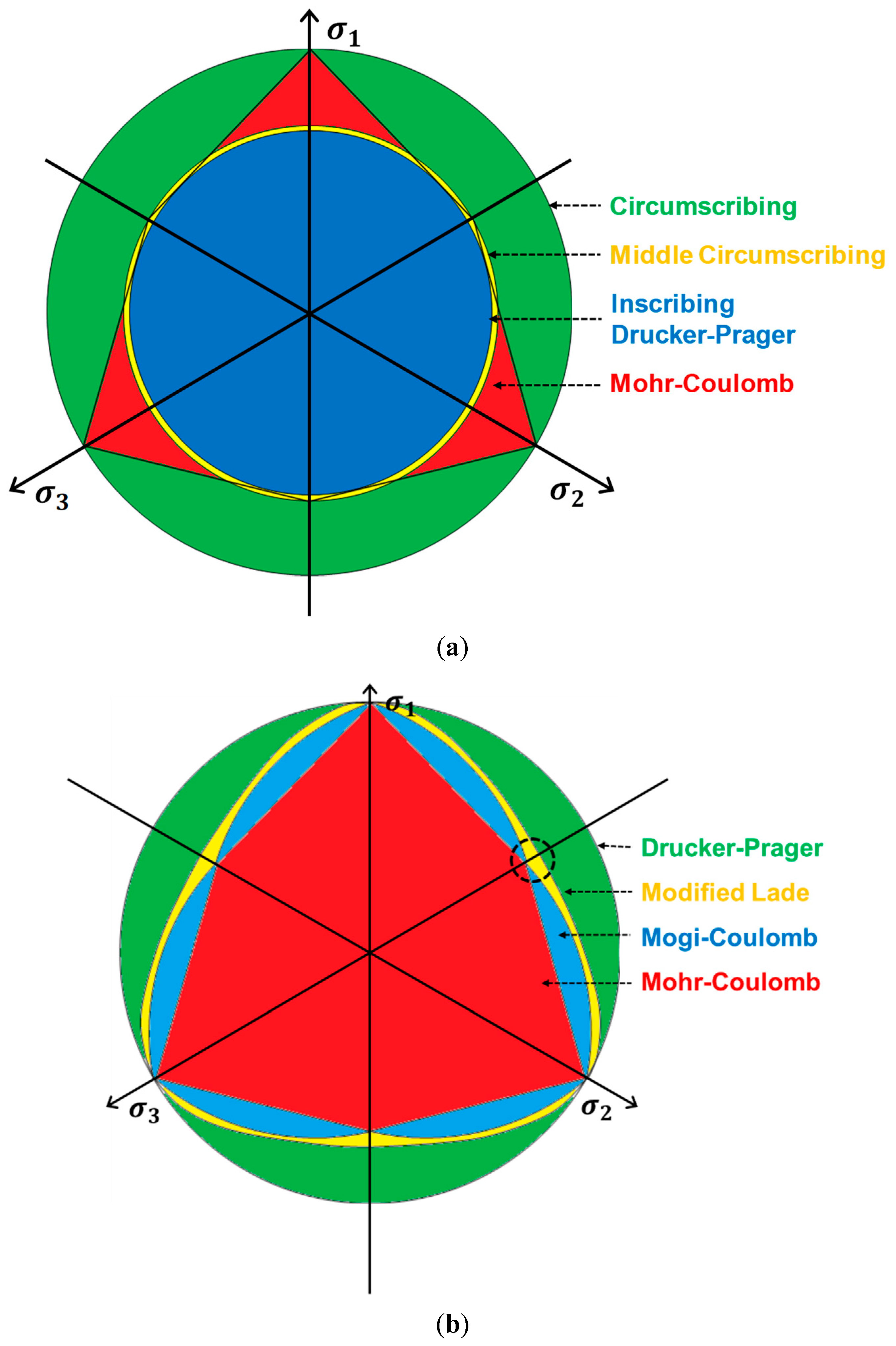
2.2. Comparison of Failure Criteria
3. Wellbore Stability Analysis Using Different Failure Criteria
3.1. Compressional Basin (Reverse Faulting) Case
3.2. Strike-Slip Basin Case
3.3. Extensional Basin (Normal Faulting) Case
4. Wellbore Stability Model Expanded with Principal Stress Trajectories and Deviatoric Stress Magnitude Contours
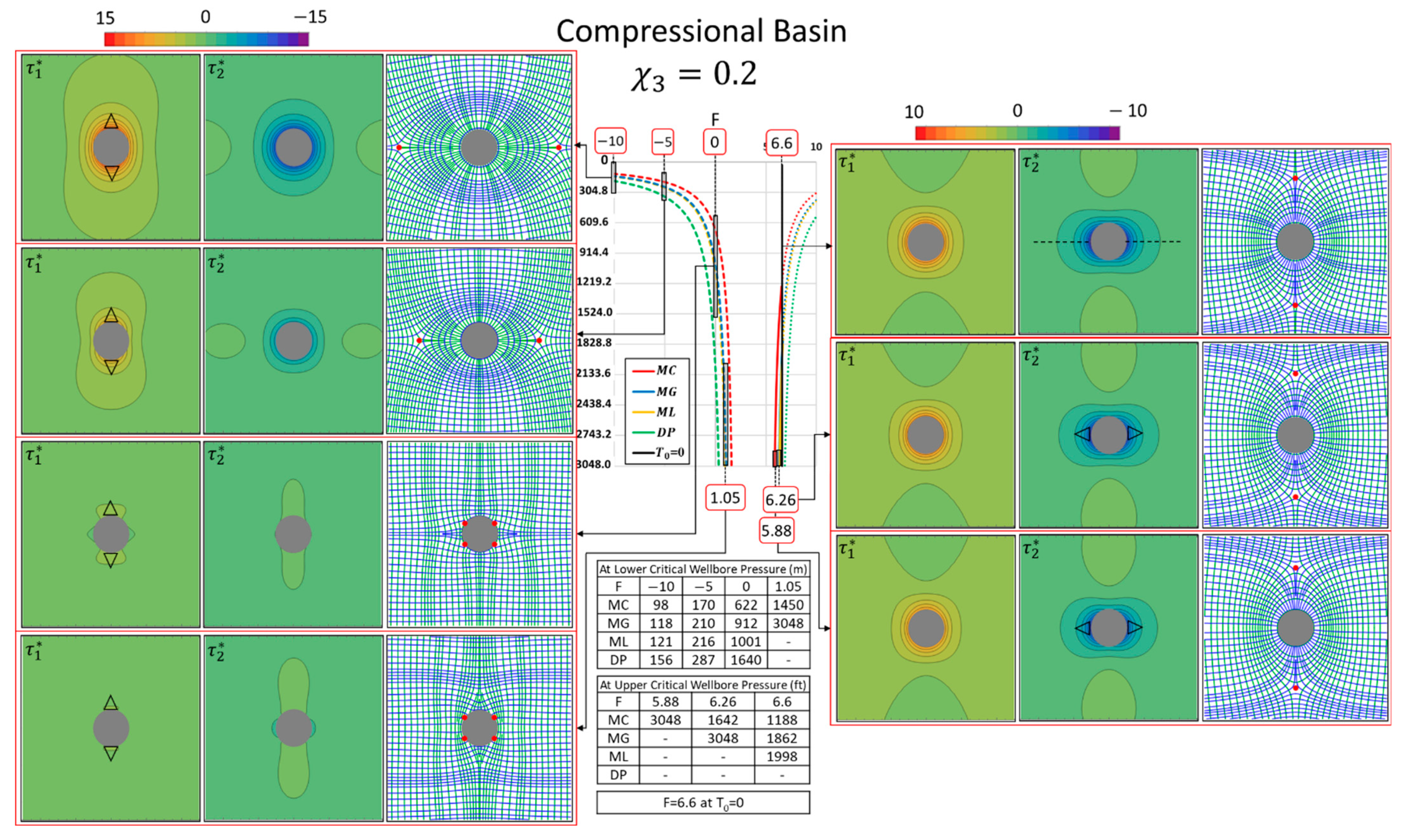
4.1. Compressional Basin Case
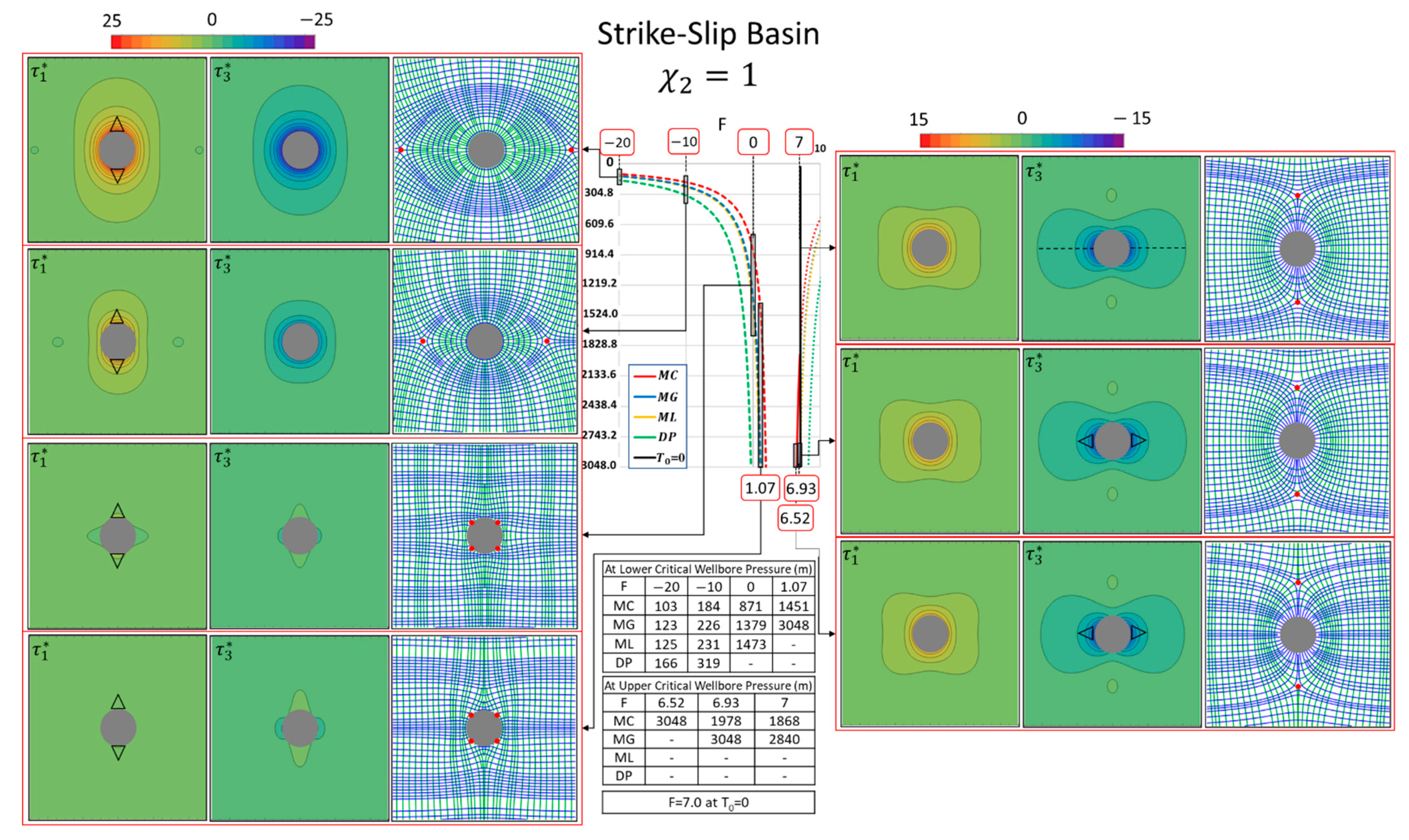
4.2. Strike-Slip Basin Case
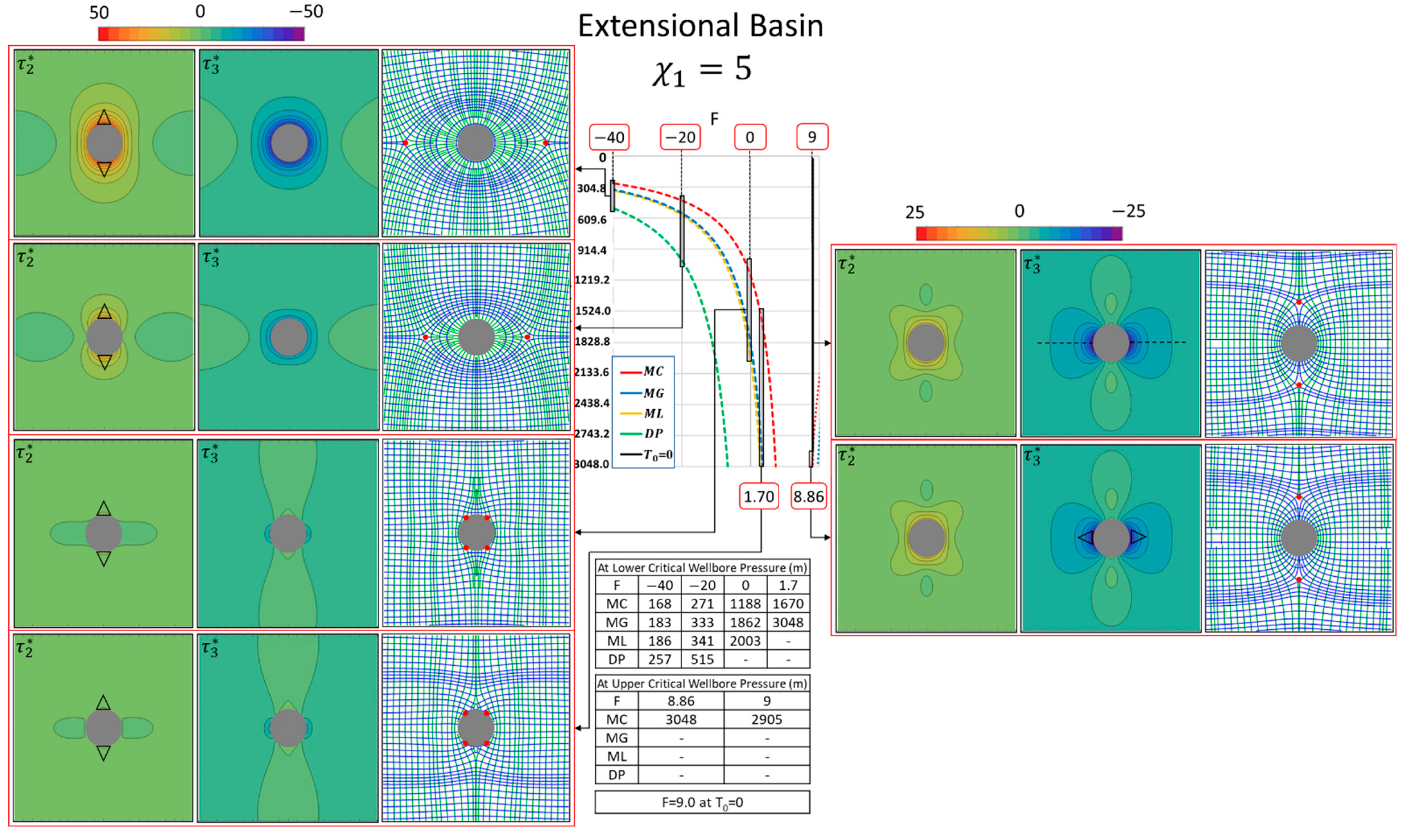
4.3. Extensional Basin Case
5. Discussion
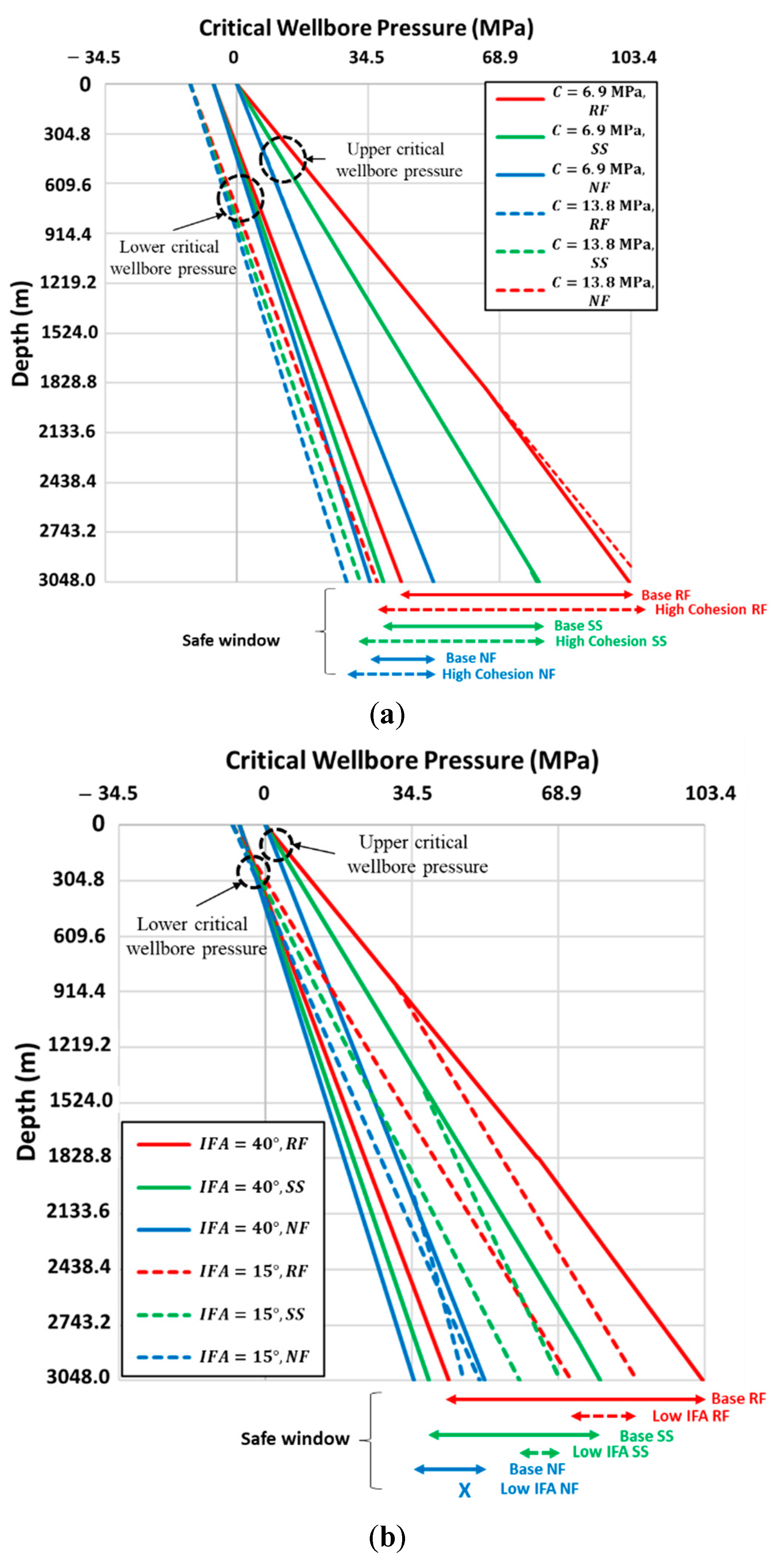
5.1. Sensitivity Analysis: Effect of Rock Strength Variations
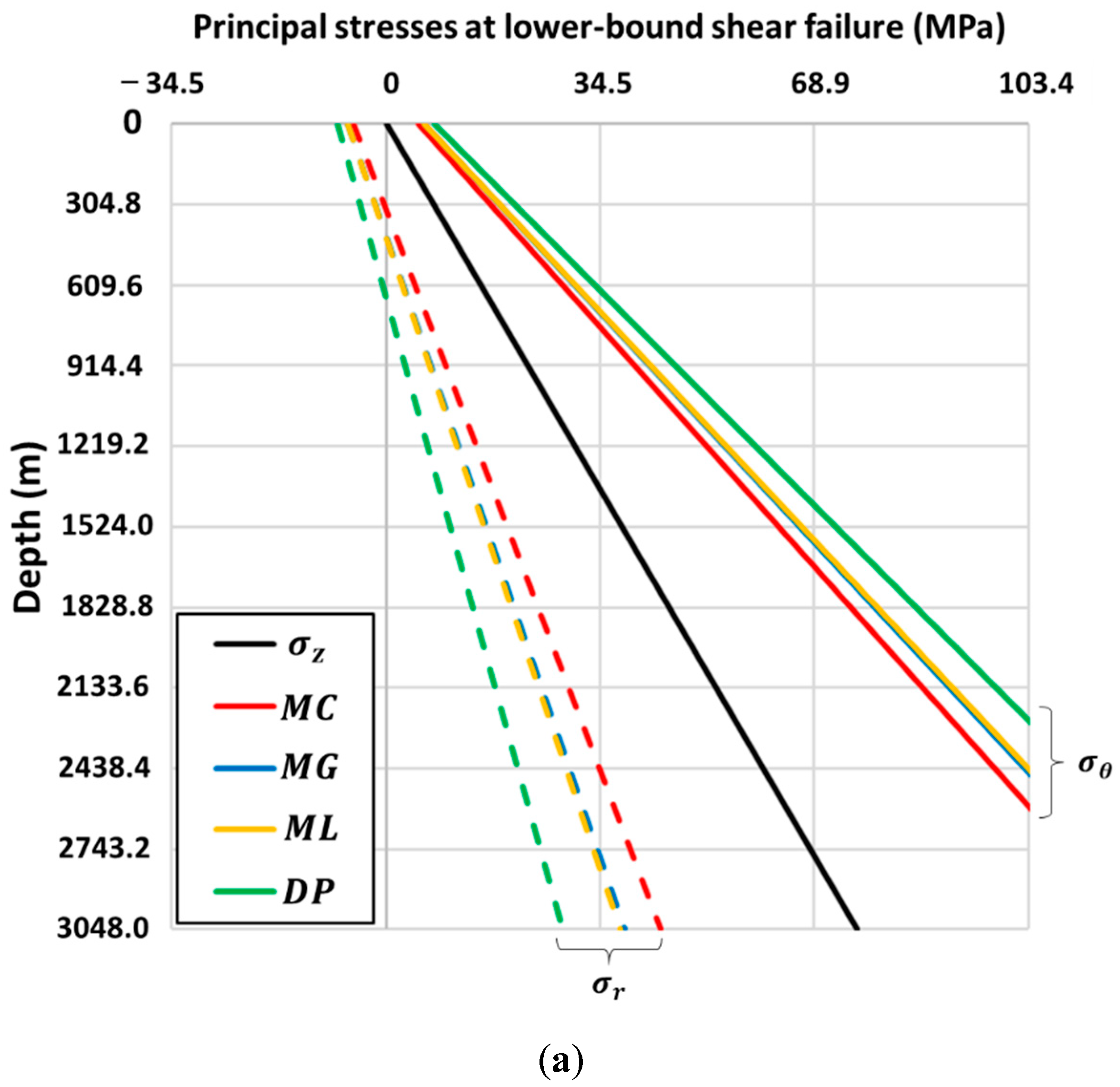
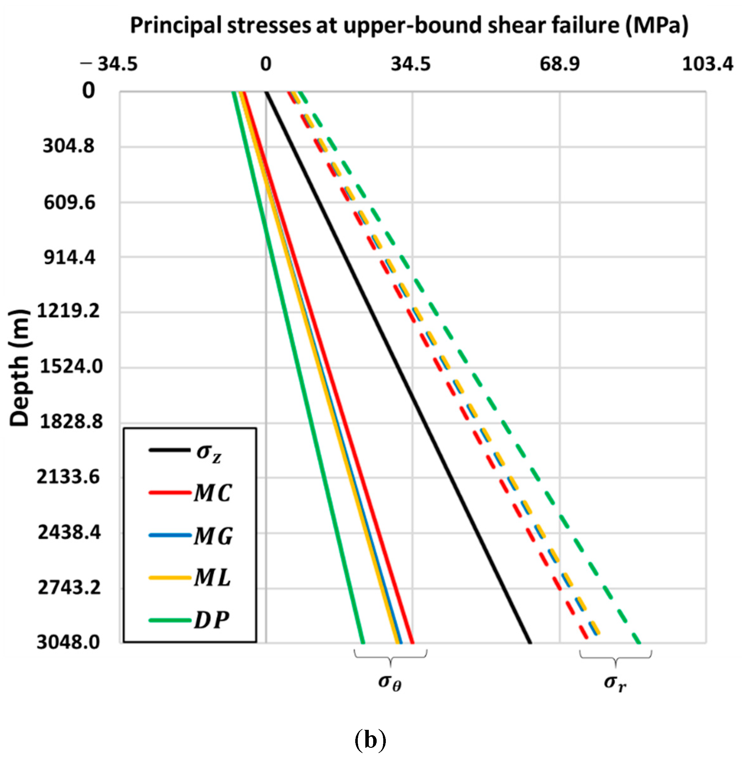
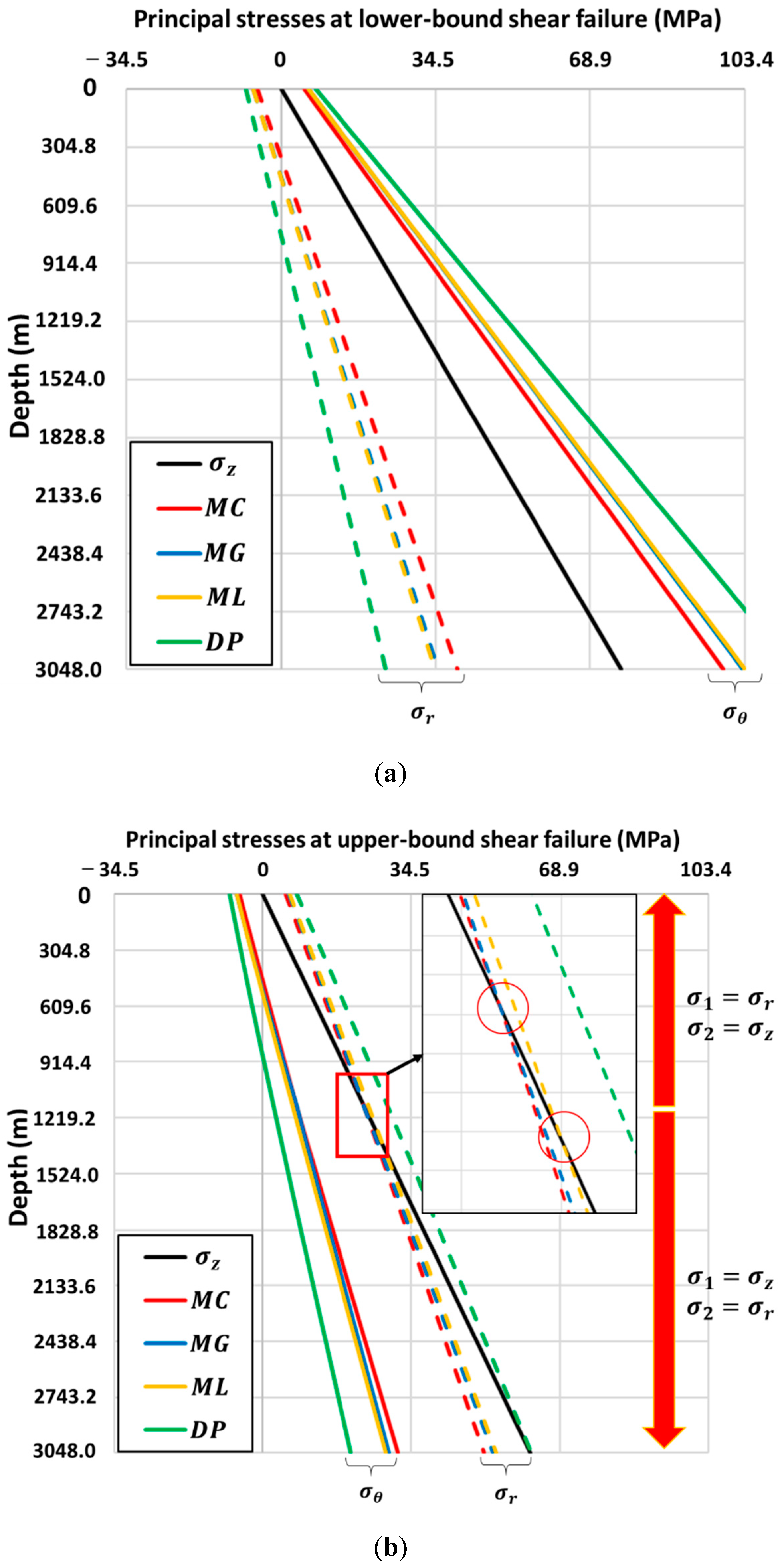
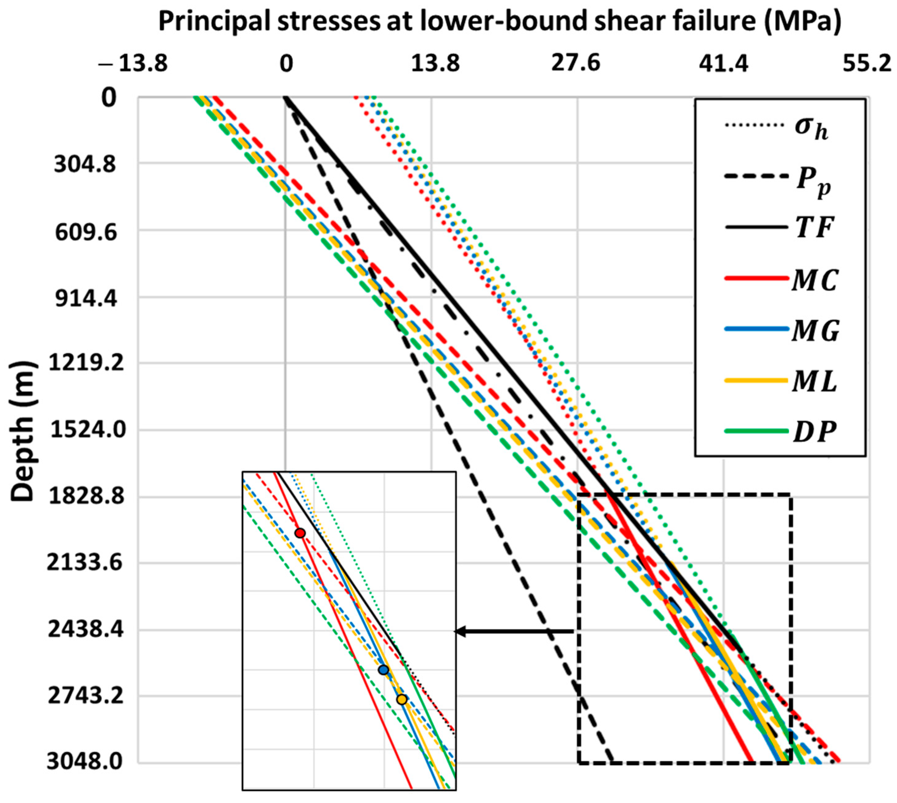
5.2. Effect of Principal Stresses at Failure Location
5.3. Importance of Stress Trajectories, Stress Cages, and Fracture Cages
- (1)
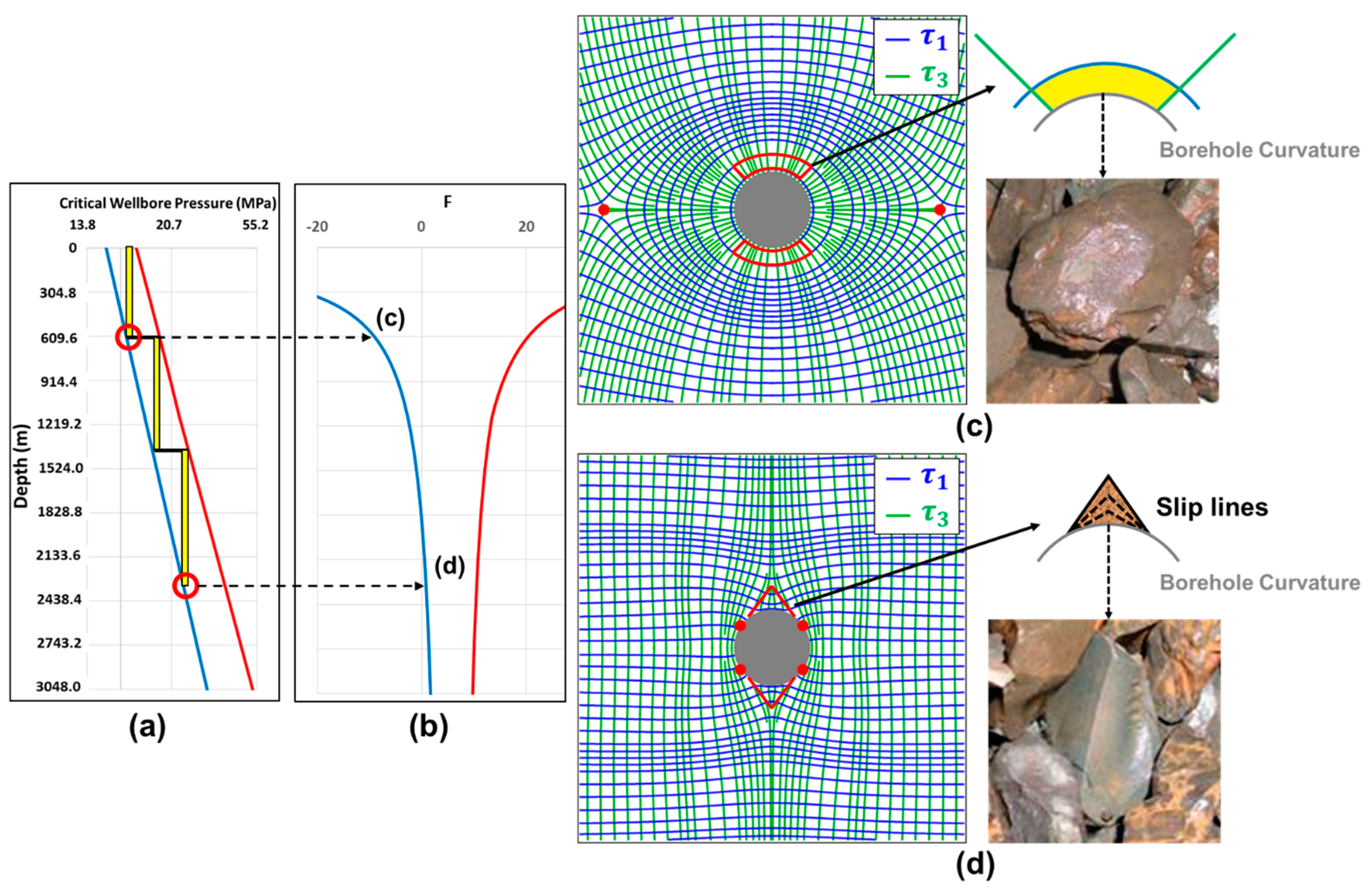
- When the radial deviatoric stress in an elliptical region near the wellbore is compressive (positive convention used here) and thus maximum, and the tangential stress is the minimum tensile stress, this is called a stress cage. The term ‘stress cage’ has been used to describe the rise in tangential stresses around a wellbore due to dilation and propping of early radial fractures [27,34,35]. According to our approach a positive Frac number is a prerequisite for the occurrence of a stress cage.
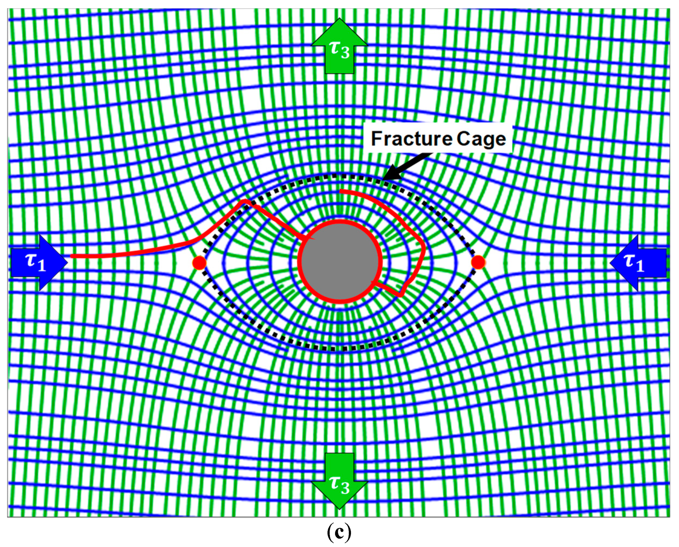
- (2)
- When the radial deviatoric stress in an elliptical region near the wellbore is tensile (negative) and thus minimum, and the tangential stress is the maximum compressive stress, this is called a fracture cage. The term was first introduced in Weijermars [30] as follows: “—Confined space around borehole where the principal deviatoric tension stress follows concentric rings so that any radial fracture emanating from the wellbore into the fracture cage space will remain trapped inside and rotate into the direction of the concentric tension rings. A negative Frac number is a prerequisite for the occurrence of a fracture cage.”
5.4. Underbalanced and Overbalanced Wellbore Pressures
5.5. Tensile Failure and Fracture Propagation
5.6. Fracture Caging and Depth
5.7. Further Work
6. Conclusions
- (1)
- At shallow depth, at the upper-bound of the safe drilling window, tensile failure is more likely to occur than shear failure. In the upper section of the well trajectory, tensile failure is triggered by lower wellbore pressures than shear failure. The traditional analysis of the safe drilling window shows that at the upper boundary, tensile failure prevails at shallower depths and shear failure prevails in deeper wells. the stress trajectories show the likely locations and propagation directions of the tensile failure and shear failure (the latter assuming transposition of stress trajectories with shear slip lines).
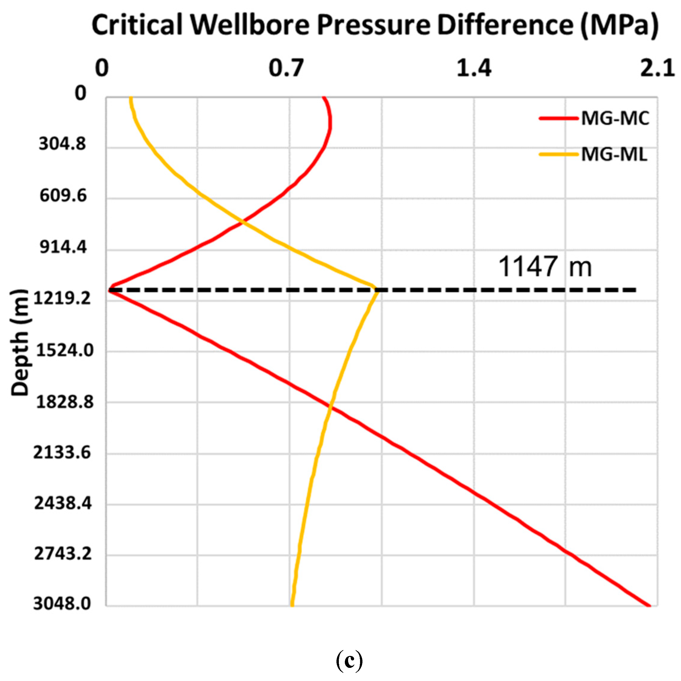
- (2)
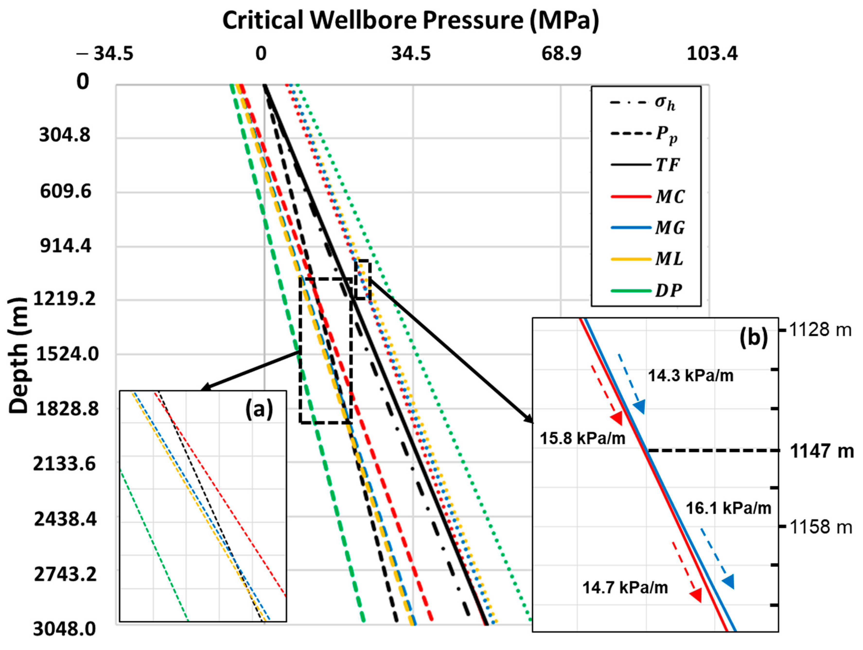
- The actual transition depth for either tensile of shear failure to prevail was evaluated for each of the three Andersonian cases and varies with the shear failure criterion used. All plausible cases have been evaluated in our study. The critical wellbore pressure gradients for both shear and tensile failure normally appear either linear or change gradually when the formation properties remain constant with depth. However, the shear failure gradient at the upper-bound of the safe window, in the extensional basin (normal faulting) case, showed a sudden change in the gradient occurs at a depth of 1147 m. According to the integrated analysis with the local principal stress states at the failure location, the change in the critical wellbore pressure gradients is caused by a reversal of the principal stress order. In all cases, our analysis shows that the locally induced principal stress condition needs to be taken into account for a more reliable wellbore stability analysis.
- (3)
- As previous studies pointed out [1], the pattern of deviatoric stress concentrations and stress trajectories near the wellbore solely depend on two dimensionless variables, the Frac number ( and the Bi-axial Stress scalar (. The range of plausible values was analyzed for three Andersonian cases (each with a fixed value). The chart is a new graphical interface that can provide valuable additional information for wellbore stability analysis, both prior to drilling and real-time during drilling operations to enhance monitoring of the well response. The examples presented in Figure 9, Figure 10 and Figure 11 show that the range of values narrows with increasing depth at the boundaries of the safe drilling window. The value at tensile failure depends on gradients of the in-situ stress and pore pressure, which are assumed constant in this study.
- (4)
- According to the magnitudes and trajectories of the maximum and minimum principal stresses, fracture caging effects are most significant for shallower wells and decreases with depth. In contrast, the stress cage effect at the upper-bound of the safe drilling window occurs at all depths in the well for each of the Andersonian cases considered here.
Supplementary Materials
Author Contributions
Acknowledgments
Conflicts of Interest
Nomenclature
| Frac number when the wellbore is aligned with (dimensionless) | |
| Mean stress (Pa) | |
| Net pressure, i.e., (Pa) | |
| Wellbore pressure (Pa) | |
| Pore pressure (Pa) | |
| Bi-axial stress scalar when the wellbore is aligned with (dimensionless) | |
| Vertical principal stress (Pa) | |
| Maximum horizontal principal stress (Pa) | |
| Minimum horizontal principal stress (Pa) | |
| Maximum principal total stress (Pa) | |
| Intermediate principal total stress (Pa) | |
| Minimum principal total stress (Pa) | |
| Total axial stress (Pa) | |
| Total radial stress (Pa) | |
| Total tangential stress (Pa) | |
| Maximum principal deviatoric stress (Pa) | |
| Intermediate principal deviatoric stress (Pa) | |
| Minimum principal deviatoric stress (Pa) | |
| Deviatoric radial stress (Pa) | |
| Deviatoric tangential stress (Pa) | |
| Deviatoric principal stress normalized by the maximum principal stress (Pa) | |
| Angle from maximum horizontal principal stress (radian) |
Appendix A. In-Situ Stress Data from Field Studies
Appendix B. Converting Non-Dimensional Stress Trajectory Scalars Using Dimensional Total Stress Inputs
Appendix B.1. Stress Trajectory Scalars Expressed in Deviatoric Stress
Appendix B.2. Conversion of Deviatoric Stresses to Total Stresses
Appendix B.3. Stress Trajectory Scalars Expressed in Total Stress: 2D Deviatoric (= Plane) Stress Cases
Appendix B.4. Intermediate Principal 3D Stress Parallel to Wellbore
Appendix B.5. Largest Principal 3D Stress Parallel to Wellbore
Appendix B.6. Minimum Principal 3D Stress Parallel to Wellbore

| Orientation Wellbore | Expressions to be Used | Value Range | |||
|---|---|---|---|---|---|
| Vertical | Horizontal | ||||
| // | // | ||||
| // | // | ||||
| // | // | ||||
Appendix B.7. Summary of Inputs and Non-Dimensionalization Algorithms to be used in our Methodology
Appendix C. Analysis of Stresses Around Wellbore
Appendix C.1. Deviatoric Stresses Around Wellbore
Appendix C.2. Stress Magnitude and Trajectory in Cartesian Coordinates
References
- Thomas, N.; Weijermars, R. Comprehensive atlas of stress trajectory patterns and stress magnitudes around cylindrical holes in rock bodies for geoscientific and geotechnical applications. Earth-Sci. Rev. 2018, 179, 303–371. [Google Scholar] [CrossRef]
- Weijermars, R.; Zhang, X.; Schultz-Ela, D. Geomechanics of fracture caging in wellbores. Geophys. J. Int. 2013, 193, 1119–1132. [Google Scholar] [CrossRef]
- Peng, S.; Zhang, J. Engineering Geology for Underground Rocks; Springer: Berlin/Heidelberg, Germany; New York, NY, USA, 2007. [Google Scholar]
- Woodland, D.C. Borehole instability in the Western Canadian overthrust belt. SPE Drill. Eng. 1990, 5, 27–33. [Google Scholar] [CrossRef]
- McLean, M.R.; Addis, M.A. Wellbore stability: The effect of strength criteria on mud weight recommendations. In SPE Annual Technical Conference and Exhibition; Society of Petroleum Engineers: New Orleans, LA, USA, 1990. [Google Scholar]
- Saberhosseini, S.E.; Ahangari, K.; Alidoust, S. Stability analysis of a horizontal oil well in a strike-slip fault regime. Aust. J. Earth Sci. 2013, 106, 137–143. [Google Scholar]
- Ramos, G.G.; Mouton, D.E.; Wilton, B.S. Integrating rock mechanics with drilling strategies in a tectonic belt, offshore Bali, Indonesia. In Proceedings of the SPE/ISRM Rock Mechanics in Petroleum Engineering, Trondheim, Norway, 8–10 July 1998; Society of Petroleum Engineers: Richardson, TX, USA, 1998. [Google Scholar]
- Onaisi, A.; Locane, J.; Razimbaud, A. Stress related wellbore instability problems in deep wells in ABK field. In Proceedings of the Abu Dhabi International Petroleum Exhibition and Conference, Abu Dhabi, UAE, 13–15 October 2000; Society of Petroleum Engineers: Richardson, TX, USA, 2000. [Google Scholar]
- Awal, M.R.; Khan, M.S.; Mohiuddin, M.A.; Abdulraheem, A.; Azeemuddin, M. A new approach to borehole trajectory optimisation for increased hole stability. In Proceedings of the SPE Middle East Oil Show, Manama, Bahrain, 17–20 March 2001; Society of Petroleum Engineers: Richardson, TX, USA, 2001. [Google Scholar]
- Willson, S.M.; Last, N.C.; Zoback, M.D.; Moos, D. Drilling in South America: A wellbore stability approach for complex geologic conditions. In Proceedings of the Latin American and Caribbean Petroleum Engineering Conference, Caracas, Venezuela, 27–29 April 1994; Society of Petroleum Engineers: Richardson, TX, USA, 1999. [Google Scholar]
- Last, N.C.; McLean, M.R. Assessing the impact of trajectory on wells drilled in an overthrust region. J. Pet. Technol. 1996, 48, 620–626. [Google Scholar] [CrossRef]
- Al-Ajmi, A.M.; Zimmerman, R.W. Stability analysis of vertical boreholes using the Mogi–Coulomb failure criterion. Int. J. Rock Mech. Min. Sci. 2006, 43, 1200–1211. [Google Scholar] [CrossRef]
- Ewy, R.T. Wellbore-stability predictions by use of a modified Lade criterion. SPE Drill. Complet. 1999, 14, 85–91. [Google Scholar] [CrossRef]
- Gholami, R.; Moradzadeh, A.; Rasouli, V.; Hanachi, J. Practical application of failure criteria in determining safe mud weight windows in drilling operations. J. Rock Mech. Geotech. Eng. 2014, 6, 13–25. [Google Scholar] [CrossRef]
- Maleki, S.; Gholami, R.; Rasouli, V.; Moradzadeh, A.; Riabi, R.G.; Sadaghzadeh, F. Comparison of different failure criteria in prediction of safe mud weigh window in drilling practice. Earth-Sci. Rev. 2014, 136, 36–58. [Google Scholar] [CrossRef]
- Meyer, J.P.; Labuz, J.F. Linear failure criteria with three principal stresses. Int. J. Rock Mech. Min. Sci. 2013, 60, 180–187. [Google Scholar] [CrossRef]
- Makhnenko, R.Y.; Harvieux, J.; Labuz, J.F. Paul-Mohr-Coulomb failure surface of rock in the brittle regime. Geophys. Res. Lett. 2015, 42, 6975–6981. [Google Scholar] [CrossRef]
- Al-Ajmi, A.M.; Zimmerman, R.W. A new well path optimization model for increased mechanical borehole stability. J. Pet. Sci. Eng. 2009, 69, 53–62. [Google Scholar] [CrossRef]
- Zhang, L.; Cao, P.; Radha, K.C. Evaluation of rock strength criteria for wellbore stability analysis. Int. J. Rock Mech. Min. Sci. 2010, 47, 1304–1316. [Google Scholar] [CrossRef]
- Fontoura, S. Lade and Modified Lade 3D Rock Strength Criteria. Rock Mech. Rock Eng. 2012, 45, 1001–1006. [Google Scholar] [CrossRef]
- Ma, T.; Chen, P.; Yang, C.; Zhao, J. Wellbore stability analysis and well path optimization based on the breakout width model and Mogi–Coulomb criterion. J. Pet. Sci. Eng. 2015, 135, 678–701. [Google Scholar] [CrossRef]
- Mansourizadeh, M.; Jamshidian, M.; Bazargan, P.; Mohammadzadeh, O. Wellbore stability analysis and breakout pressure prediction in vertical and deviated boreholes using failure criteria—A case study. J. Pet. Sci. Eng. 2016, 145, 482–492. [Google Scholar] [CrossRef]
- Das, B.; Chatterjee, R. Wellbore stability analysis and prediction of minimum mud weight for few wells in Krishna-Godavari Basin, India. Int. J. Rock Mech. Min. Sci. 2017, 93, 30–37. [Google Scholar] [CrossRef]
- Abbasi, S.; Singh, R.K.; Singh, K.H.; Singh, T.N. Selection of failure criteria for estimation of safe mud weights in a tight gas sand reservoir. Int. J. Rock Mech. Min. Sci. 2018, 107, 261–270. [Google Scholar] [CrossRef]
- Weijermars, R. Analytical stress functions applied to hydraulic fracturing: Scaling the interaction of tectonic stress and unbalanced borehole pressures. In Proceedings of the 45th U.S. Rock Mechanics/Geomechanics Symposium, San Francisco, CA, USA, 26–29 June 2011; American Rock Mechanics Association: Alexandria, VA, USA, 2011. [Google Scholar]
- Thomas, N. Visualizing Wellbore Instability and Planes of Failure in Boreholes by Application of Principal Stress Trajectory Analysis. Master’s Thesis, Texas A&M University, College Station, TX, USA, 2017. [Google Scholar]
- Alberty, M.W.; McLean, M.R. A Physical Model for Stress Cages. In Proceedings of the SPE Annual Technical Conference and Exhibition, Houston, TX, USA, 26–29 September 2004; Society of Petroleum Engineers: Richardson, TX, USA, 2004. [Google Scholar]
- Chang, C.; Zoback, M.D.; Khaksar, A. Empirical relations between rock strength and physical properties in sedimentary rocks. J. Pet. Sci. Eng. 2006, 51, 223–237. [Google Scholar] [CrossRef]
- McLean, M.R.; Addis, M.A. Wellbore stability analysis: A review of current methods of analysis and their field application. In Proceedings of the SPE/IADC Drilling Conference, Houston, TX, USA, 27 February–2 March 1990; Society of Petroleum Engineers: Richardson, TX, USA, 1990. [Google Scholar]
- Weijermars, R. Mapping stress trajectories and width of the stress-perturbation zone near a cylindrical wellbore. Int. J. Rock Mech. Min. Sci. 2013, 64, 148–159. [Google Scholar] [CrossRef]
- Pašić, B.; Gaurina-Međimurec, N.; Matanović, D. Wellbore instability: Causes and consequences. Rud. Geološko Naft. Zb. 2007, 19, 87–98. [Google Scholar]
- Bowes, C.; Procter, R. Drillers Stuck Pipe Handbook; Schlumberger: Ballater, UK, 1997. [Google Scholar]
- Weijermars, R. Stress cages and fracture cages in stress trajectory models of wellbores: Implications for pressure management during drilling and hydraulic fracturing. J. Nat. Gas Sci. Eng. 2016, 36, 986–1003. [Google Scholar] [CrossRef]
- Wang, H.; Soliman, M.Y.; Towler, B.F. Investigation of Factors for Strengthening a Wellbore by Propping Fractures. In Proceedings of the IADC/SPE Drilling Conference, Orlando, FL, USA, 4–6 March 2008; Society of Petroleum Engineers: Richardson, TX, USA, 2008; p. 15. [Google Scholar]
- Tovar, J.; Bhat, S. Characterization of Stress Caging Effect for Resolving Wellbore Integrity Problems in Fractured Formations—Experimental Results. VII INGEPET 2011 (EXPL-2-JT-02). 2011. Available online: https://www.researchgate.net/publication/281902738_CHARACTERIZATION_OF_THE_STRESS_CAGING_EFFECT_FOR_RESOLVING_WELLBORE_INTEGRITY_PROBLEMS_IN_FRACTURED_FORMATIONS_-_EXPERIMENTAL_RESULTS (accessed on 30 June 2019).
- Zhang, X.; Jeffrey, R.G.; Bunger, A.P. Hydraulic Fracture Growth From a Non-Circular Wellbore. In Proceedings of the 45th U.S. Rock Mechanics/Geomechanics Symposium, San Francisco, CA, USA, 26–29 June 2011; American Rock Mechanics Association: Alexandria, VA, USA, 2011; p. 9. [Google Scholar]
- Li, Y.; Weijermars, R. Wellbore stability analysis in transverse isotropic shales with anisotropic failure criteria. J. Pet. Sci. Eng. 2019, 176, 982–993. [Google Scholar] [CrossRef]
- Weijermars, R.; Wang, J.; Nelson, R. Elastic anisotropy in shale formations and its effect on near-borehole stress fields and failure modes. Earth-Sci. Rev. 2019, in press. [Google Scholar] [CrossRef]
- Wang, J.; Weijermars, R. Expansion of Horizontal Wellbore Stability Model for Elastically Anisotropic Shale Formations With Anisotropic Failure Criteria: Permian Basin Case Study. In Proceedings of the 53rd U.S. Rock Mechanics/Geomechanics Symposium, New York, NY, USA, 23–26 June 2019; American Rock Mechanics Association: Alexandria, VA, USA, 2019. [Google Scholar]
- Klee, G.; Rummel, F.; Williams, A. Hydraulic fracturing stress measurements in Hong Kong. Int. J. Rock Mech. Min. Sci. 1999, 36, 731–741. [Google Scholar] [CrossRef]
- Kirsch, G. Die theorie der elastizität und die bedürfnisse der festigkeitslehre. Z. Ver. Dtsch. Ing. 1898, 42, 797–807. [Google Scholar]
- Zoback, M.D.; Barton, C.A.; Brudy, M.; Castillo, D.A.; Finkbeiner, T.; Grollimund, B.R.; Moos, D.B.; Peska, P.; Ward, C.D.; Wiprut, D.J. Determination of stress orientation and magnitude in deep wells. Int. J. Rock Mech. Min. Sci. 2003, 40, 1049–1076. [Google Scholar] [CrossRef]


| Location | Western Canada | Cyrus Reservoir, UK | Mansouri Field, Iran | Pagerungan Island, Indonesia | ABK field, Abu-Dhabi | Offshore Wells, Arabian Gulf | Cusiana Field, Columbia | Cusiana Field, Columbia |
|---|---|---|---|---|---|---|---|---|
| Source | [4] | [5] | [6] | [7] | [8] | [9] | [10] | [11] |
| Andersonian Type | Strike-slip | Extensional | Strike-slip | Strike-slip | Compressional | Extensional | Strike-slip | Strike-slip |
| Depth (m) | >3048 | 2600 | 2313 | 1463–1890 | 2958 | 2073 | 4572 | 3048 |
| gradient (kPa/m) | 24.9 ± 0.7 | 22.6 | 25.3 | 22.6 | 22.6 | 24.9 | 24.4 | 24.9 |
| gradient (kPa/m) | 28.0 | 17.0 | 27.6 | 27.6 | 34.4 | 22.6 | 30.8 | 31.7 |
| gradient (kPa/m) | 19.2 ± 1.4 | 17.0 | 14.3 | 19.7 | 24.4 | 20.4 | 17.0 | 15.8 |
| gradient (kPa/m) | 9.7 | 10.2 | 9.3 | 10.2 | 10.2 | 10.4 | 9.5 | 10.0 |
| (MPa) | - | - | 27.8 | 47.7 | 5.5 | 21.3 | 70.0 | - |
| Cohesion (MPa) | - | 5.9 | 5.4 | 12.4 | - | 6.0 | 19.8 | - |
| Tensile Strength (MPa) | - | - | 2.0 | - | - | - | - | - |
| Internal Friction Angle (°) | - | 43.8 | - | 35.0 | 50.2 | 31.3 | 31.0 | - |
| Poisson’s Ratio | - | 0.18 | 0.20 | 0.30 | - | - |
| Andersonian Type | Compressional | Strike-Slip | Extensional |
|---|---|---|---|
| gradient (kPa/m) | 22.6 | 22.6 | 22.6 |
| gradient (kPa/m) | 29.4 | 24.9 | 20.4 |
| gradient (kPa/m) | 24.9 | 20.4 | 15.8 |
| 0.20 | 1.00 | 5.00 | |
| gradient (kPa/m) | 10.2 | ||
| Cohesion (MPa) | 6.9 | ||
| Internal Friction Angle (°) | 40.00 | ||
| Unconfined Compressive Strength (MPa) | 29.6 | ||
| Poisson’s ratio | 0.25 | ||
| Andersonian Case | Spatially Fixed Subscripts | ||
|---|---|---|---|
| Compressional Basin | |||
| Extensional Basin | |||
| Strike Slip Basin | |||
| Principal Total Stress Subscripts (all cases) | |||
| Principal Deviatoric Stress Subscripts (all cases) | |||
| Andersonian Type | Compressional (m) | Strike-Slip (m) | Extensional (m) |
|---|---|---|---|
| Mohr–Coulomb | 688 | 872 | 1188 |
| Mogi–Coulomb | 1035 | 1379 | 1862 |
| Modified Lade | 1128 | 1470 | 2002 |
| Drucker–Prager | 2109 | - | - |
© 2019 by the authors. Licensee MDPI, Basel, Switzerland. This article is an open access article distributed under the terms and conditions of the Creative Commons Attribution (CC BY) license (http://creativecommons.org/licenses/by/4.0/).
Share and Cite
Wang, J.; Weijermars, R. New Interface for Assessing Wellbore Stability at Critical Mud Pressures and Various Failure Criteria: Including Stress Trajectories and Deviatoric Stress Distributions. Energies 2019, 12, 4019. https://doi.org/10.3390/en12204019
Wang J, Weijermars R. New Interface for Assessing Wellbore Stability at Critical Mud Pressures and Various Failure Criteria: Including Stress Trajectories and Deviatoric Stress Distributions. Energies. 2019; 12(20):4019. https://doi.org/10.3390/en12204019
Chicago/Turabian StyleWang, Jihoon, and Ruud Weijermars. 2019. "New Interface for Assessing Wellbore Stability at Critical Mud Pressures and Various Failure Criteria: Including Stress Trajectories and Deviatoric Stress Distributions" Energies 12, no. 20: 4019. https://doi.org/10.3390/en12204019
APA StyleWang, J., & Weijermars, R. (2019). New Interface for Assessing Wellbore Stability at Critical Mud Pressures and Various Failure Criteria: Including Stress Trajectories and Deviatoric Stress Distributions. Energies, 12(20), 4019. https://doi.org/10.3390/en12204019