Article

The Effect of Collector Shading and Masking on Optimized PV Field Designs

School of Electrical Engineering, Tel Aviv University, Tel Aviv 69978, Israel
*
Author to whom correspondence should be addressed.
Energies 2019, 12(18), 3471; https://doi.org/10.3390/en12183471
Submission received: 30 July 2019 / Revised: 4 September 2019 / Accepted: 6 September 2019 / Published: 9 September 2019
(This article belongs to the Special Issue PV Systems: from Small- to Large-Scale)

Abstract

:
Photovoltaic (PV) solar fields are deployed with multiple rows. The second and subsequent rows are subject to shading and masking by the rows in front. The direct beam incident radiation on the second row is affected by shading and the diffuse incident radiation is affected by masking, expressed by sky view factor. Hence, all rows, besides the first one, receive lower incident radiation. The design of PV fields must take into account the decrease in the incident radiation caused by these two effects. The paper investigates by simulation the annual incident diffuse, direct beam and global radiation on the first and on the second row for optimized PV fields at two sites: Tel Aviv, Israel, with low diffuse component, and Lindenberg–Germany monitoring station, with a high diffuse component. The study emphasizes the importance of the diffuse incident radiation on the energy loss of the PV field. The percentage annual global energy loss due to shading and masking on the second row amounts to 1.49% in Tel Aviv and 0.46% in Lindenberg. Isotropic and anisotropic diffuse models were considered. The calculated diffuse incident energy for the isotropic model is lower than the values for anisotropic model by about 8% in Tel Aviv and 3.75% in Lindenberg.

1. Introduction

Photovoltaic (PV) collectors are usually deployed in a number of rows facing south (in the northern hemisphere) on horizontal or on inclined planes. The second and subsequent collector rows are subject to shading and masking (expressed by the sky view factor) by the rows in front. Shading affects the direct beam radiation [1,2] and masking affects the diffuse incident radiation on the rows [3]. A design of PV fields must take into account the decrease in the incident radiation caused by these two effects and hence causing losses in the electrical energy generation. Shading of different kinds on PV modules is considered an adversary to PV systems and mitigating means were devised to reduce its effect, such as increasing the collectors’ row-to-row distance and including bypass diodes in the PV modules. Not much attention has been paid in the past to the masking phenomenon and its effect on the power loss of PV systems. In fact, the amount of masking on the collector varies along the collector width causing uneven incident diffuse radiation on the PV modules. The detrimental effect associated with masking has been addressed in a recent work which established the view-factor as an emerging topic of technical significance [3]. The article deals with the effect of uneven diffuse incident radiation on the PV cells within the module caused by the effect of the local view factor along the module’s surface. The uneven diffuse radiation inflicts current mismatch between the strips of the module, manifesting by step formation on the I–V characteristic and affecting the output power of the module. The present study investigates the annual incident diffuse, direct beam and global radiation on the first and on the second row for optimized PV fields. An optimal design of a PV field may be formulated mathematically as a constrained optimization problem comprising of an objective function and a set of constraints usually multivariable and nonlinear in both the objective and constraint functions [4,5]. Based on this mathematical concept, optimal PV systems were formulated and studied in [6,7,8]. These articles consider row shading and masking in the optimal designs and employ the isotropic diffuse radiation model. Articles dealing with optimal designs of PV systems for different objective functions and different optimization algorithms are mentioned in [7]. The present study widened the optimal design of PV fields not dealt with in References [6,7] by including designs on inclined fields in Tel Aviv, Israel (latitude 32° N) with low diffuse radiation component and in Lindenberg, Germany (latitude 52.2° N) with high diffuse radiation component, for both horizontal and inclined fields. In addition, the effect of isotropic and anisotropic diffuse radiation models on the design is compared in the study. The study emphasizes the importance of the incident diffuse radiation (associated with the sky view factor) on the energy loss of the PV field. The energy loss due to shading and masking may be translated into de-rated power of the PV module and therefore has significant technical consequences for PV field designs.

2. Materials and Methods

2.1. Diffuse Radiation Models

The diffuse radiation from the whole sky-dome is highly variable and therefore a large number of diffuse radiation models have been proposed. For comparing the effect of the diffuse radiation on the PV system design, the present study employed the isotropic model by Liu and Jordan [9], and the anisotropic (“all sky”) model by Klucher [10]. The solar spectrum of the direct beam radiation and the sky diffuse radiation are different, therefore affect the generated output power of PV cells differently. For the sake of simplicity, the spectrum variation during the day for the direct beam and diffuse radiation is not considered in the present study.

2.2. Isotropic Diffuse Model

The global solar irradiance G incident on a PV module, neglecting the reflected irradiances, consisted of the direct beam irradiance G b and the diffuse irradiance G d . The diffuse irradiance consisted of the diffuse irradiance G d h on a horizontal plane and the sky view factor F:
G = G b + G d = G b + F G d h .
Analytical expressions for the sky view factor for PV fields in multiple rows were developed in [6,7]. The sky view factor for a single row or for the first row in a multiple row field of stationary collectors on horizontal grounds was given by [9]:
F = ( 1 + cos β ) / 2
and the sky view factor for a row on an inclined plane was given by:
F = [ 1 + cos ( β ε ) ] / 2 ,
where β is the inclination angle of the row to a horizontal plane and ε is the inclination angle of the plane, see Figure 1 and Figure 2.
The length of the row is much larger than its width, therefore the calculation of view factors, for the second and subsequent rows, may be based on the “cross-string rule” [11,12]. In the present study the “cross-string rule” was used since it is simple to apply.
The view factor is a numerical value expressed by the geometry of the row and the distance between the rows, Figure 1 and Figure 2. Based on the “cross-string rule”, the sky view factor of the second and subsequent rows on a horizontal plane is given by:
F = 2 H + D + 2 H cos β [ D 2 + ( 2 H sin β ) 2 ] 1 / 2 4 H ,
and on an inclined plane ε is given by:
F = 2 H + [ ( D + 2 H cos β ) 2 + B 2 ] 1 / 2 [ D 2 + ( 2 H sin β B ) 2 ] 1 / 2 4 H
where (see Figure 2)
B = ( D + 2 H cos β ) tan ε .
A general expression for the sky view factor developed in [3] pertains to any number N of PV cell rows in a module. Therefore, this expression may also apply to rows in a PV field containing N modules placed one above the other along the row width. For simplicity, the present study assumes N = 2 for all the studied cases.

2.3. Anisotropic Diffuse Model

The Klucher model for diffuse radiation (“all sky” anisotropic model) is given by:
G d = F G d h ( 1 + F K cos 2 θ sin 3 θ Z ) ( 1 + F K sin 3 β 2 ) ,
where
F K = 1 G d h G g h = G g h G d h G g h .
G g h is the global radiation on a horizontal surface, θ is the angle between the beam irradiance on the surface and the normal to that surface and θ Z is the solar zenith angle.

2.4. Formulation of the Optimal Design of a PV Field

Photovoltaic fields are usually designed optimally meeting some economic or energy objectives, such as obtaining maximum incident energy from a given field, minimum cost per unit energy, etc. The optimal design of a solar field may be formulated mathematically as a constrained optimization problem comprising of an objective function and a set of constraints [6]. The problem variables include field and collector parameters: field length L; field width W; distance between collector rows D; collector width 2H; inclination angle β ; number of collector rows K, and geometric limits of these parameters. The constraints were bounding conditions imposed on the design parameters. In the present study, the maximum incident energy on the PV field was the objective function considering shading and masking. The methodology for calculating the incident energies (beam, diffuse and global) was presented in Reference [6].

2.4.1. Maximum Annual Incident Energy-Horizontal Field

Defining the objective function as maximum annual incident energy on the PV field of given dimensions L max × W max ( L max —field length, W max —field width), the optimization problem is formulated as follows:
Maximize energy E: C ( X ¯ ) with respect to vector parameters X ¯ = ( D , β , K ) ,
Subject to (see Figure 1):
2 H × K × cos β + ( K 1 ) × D W max K 2 ,    0 ° β 90 ° .
The distance D between the collector rows depended on the inclination angle β and on the collector width 2H, and was determined by the shadow length cast by the first row on the ground for sun elevation angle on 21 December at solar noon (in the northern hemisphere):
D ( 2 H , β ) = 2 H sin β tan [ sin 1 ( cos ( ϕ δ 0 ) ] ,
where ϕ is the site’s latitude and δ 0 = 23.45 ° is earth’s declination angle at winter solstice.
The distance D affected the shading and masking and hence affected the incident radiation on the PV modules. It is therefore customary to select the distance D (Equation (10) as a basis for comparing different PV fields (see the discussion section). The view factors are given in Equation (2) for the first row and in Equation (4) for the second and subsequent rows.

2.4.2. Maximum Annual Incident Energy-Inclined Field

Defining the objective function as maximum annual incident energy on the PV field deployed on an inclined field ε of give dimensions L max × W max , the optimization problem was formulated as follows:
Maximize energy E: C ( X ¯ ) with respect to vector parameters X ¯ = ( D , β , K ) ,
Subject to (see Figure 2):
2 H × K × cos β + ( K 1 ) × D W max K 2 ,    ε ° β 90 ° .
The view factors are given in Equation (3) for the first collector row and in Equation (5) for the second and subsequent rows.
The distance D between the collector rows was determined by:
D ( 2 H , β ) = 2 H sin β B tan [ sin 1 ( cos ( ϕ δ 0 ) ] ,
where B for an inclined plane is given in Equation (6).

3. Results

3.1. Optimization Results: Horizontal Field–Isotropic Model—Tel Aviv

The objective is to calculate the annual incident diffuse, direct beam and global energy on the first and on the second row for an optimized PV field, and to study the sensitivities of these energies to row distance and to the inclination angle. The optimal design pertains to Tel Aviv—latitude 32° N, 10 min solar radiation data), with relatively low percentage diffuse radiation. The PV module and field dimensions are, respectively: H = 0.941/m, L = 100/m, W = 100/m and are a design basis for all following cases.
The energies of the optimal design for Tel Aviv are summarized in Table 1. The optimal inclination angle is β = 16.55 ° , the field contains K = 38 rows, and the distance between the rows is D = 0.85 m. The view factors of the first, Equation (2) and second row, Equation (4) are F 1 = 0.978 and F 2 = 0.934 , respectively. The annual incident energy of the whole PV field (38 rows) is denoted by E y , the annual diffuse incident energy on the first collector row is E d 1 , and on the second row is E d 2 ; the annual beam incident energy on first collector row is E b 1 ; and on the second row is E b 2 ; the annual global incident energy on the first collector row is E G 1 ; and on the second row is E G 2 . The results for the subsequent rows are the same as for the second row. The field width W is fully utilized (K is rounded off to a whole number).
Based on the results in Table 1, the following conclusions reveal that:
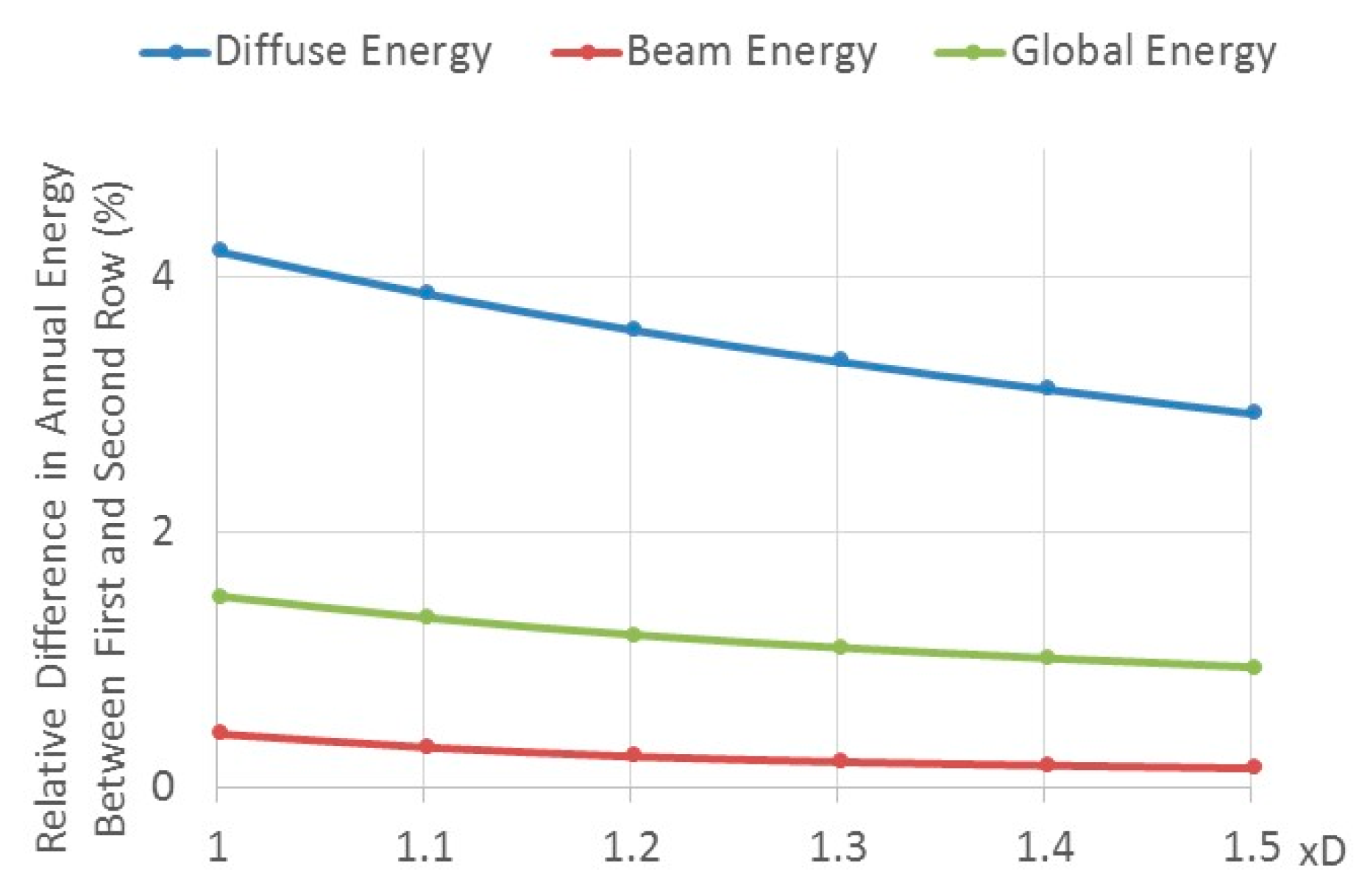
  • The percentage annual energy loss due to shading (beam) on the second row (cast by the collector in front) amounts to 0.42%.
  • The percentage annual energy loss due to masking (diffuse) on the second row (caused by the collector in front) amounts to 4.2%.
  • The percentage annual global energy loss due to shading and masking on the second row (caused by the collector in front) amounts to 1.49%.
  • The incident diffuse radiation on the second and subsequent collector rows dominates the energy loss of the whole PV field.
Of interest may be the sensitivities of the above results to variation in the distance between the rows D. Figure 3 shows the relative difference in the annual incident energy (diffuse, beam and global) between the first and second row for distances between 1.0 (0.85/m) to 1.5 times D (1.275/m), for β = 16.55 ° , K = 38 (optimal results). Increasing the row distance has little effect on the global incident energy of the PV field. On the other hand, for a given field width W, the number of rows will decrease and hence affecting adversely the PV field generated energy.
The sensitivity of the inclination angle β to the energy (diffuse, beam and global) is depicted in Figure 4 for Tel Aviv. The relative difference of annual incident energy between the first and second row increases as the inclination angle increases. Larger inclination angles increase the mutual shading (beam) between the rows, and decrease the sky view factor, causing larger masking (diffuse) between the rows.

3.2. Optimization Results: Horizontal Field–Anisotropic Model—Tel Aviv

The isotropic diffuse model by Liu–Jordan underestimates the amount of diffuse radiation falling on inclined planes compared to anisotropic diffuse model by Klucher [10] as we will see also in the present study. The energy of the optimal design results applying the Klucher diffuse model is summarized in Table 2.
The optimal inclination angle is β = 14.33 ° ; the field contains K = 38 rows; the distance between the rows is D = 0.83 / m . The anisotropic diffuse model results in 112,432/kWh (Table 2) as compared to 102,975/kWh (Table 1) for the isotropic model for the first row, and 107,178/kWh (anisotropic model) compared to 98,646/kWh (isotropic model) for the second row, an increase of about 8%. The optimization results using the anisotropic diffuse model are different respectively, obtaining, for example, 1.91% more annual global incident energy E y of the whole PV field.

3.3. Optimization Results: Inclined Field–Isotropic Model—Tel Aviv

The optimal results for the PV system for field inclination angles ε = 0°, 5° and 10° are summarized in Table 3. Table 3 shows that the annual incident global field energy, the row inclination angle β , and the number of rows K increase with the increase of the field inclination angle ε . The field width W is utilized in full (K is rounded off to a whole number). The second row receives less incident energies (beam, diffuse and global) than the first row; the amounts may be derived from Table 3.

3.4. Optimization Results: Horizontal Field–Isotropic Model—Lindenberg

The objective is to calculate the annual incident energy on the first and on the second row for an optimized PV field, and to study the sensitivity of the energy to row distance and inclination angle. The optimal design pertains to Lindenberg, Germany, with a high percentage of diffuse radiation, latitude 52.2° N (Meteorologisches Observatorium Lindenberg, Richard-Aßmann-Observatorium, PANGAEA, Monitoring station no. 12, BSRN-https://dataportals.pangaea.de/bsrn/?q=LR1300, Ten minutes of solar radiation data, year 2006). The energy of the optimal design for Lindenberg is summarized in Table 4. The optimal inclination angle is β = 6.68 ° , the field contains K = 37 rows, and the distance between the rows is D = 0.86 /m. The view factors of the first, Equation (2) and second row are F 1 = 0.995 and F 2 = 0.984 , respectively. Based on the results in Table 4, the following conclusions reveal that: the percentage annual energy loss due to shading and masking amounts to 0.18% and 0.73%, respectively, and percentage of global energy loss is 0.46% between the first and the second row.
The sensitivities of the above results to variation in distance between the rows are shown in Figure 5. The figure shows the relative difference in the annual incident energy (diffuse, beam and global) between the first and second row for distances between 1.0 (0.86/m) to 1.5 times D (1.29/m), for β = 6.68 ° , K = 37 (optimal results). Increasing the row distance has little effect on the global incident energy of the PV field.
The sensitivity of the inclination angle β to the energy (diffuse, beam and global) is depicted in Figure 6 for Lindenberg. The relative difference of the annual incident energy between the first and second row increases as the inclination angle increases. Larger inclination angles increase the mutual shading (beam) between the rows, and decrease the sky view factor, causing larger masking (diffuse) between the rows.

3.5. Optimization Results: Horizontal Field–Anisotropic Model—Lindenberg

The energy of the optimal design results applying Klucher diffuse model are summarized in Table 5. The optimal inclination angle is β = 6.68 ° , the field contains K = 37 rows, and the distance between the rows is D = 0.86 /m remained all the same as for the isotropic model; however, the incident solar radiation is different. The anisotropic diffuse model results in 109,492/kWh (Table 5) as compared to 105,349/kWh (Table 4) for the isotropic model for the first collector row, and 108,594/kWh (anisotropic model) as compared to 104,575/kWh (isotropic model) for the second row, an increase of about 3.7%. The optimization results using the anisotropic diffuse model are different respectively, obtaining, for example, 1.87% more annual global incident energy E y of the whole PV field.

3.6. Optimization Results: Inclined Field–Isotropic Model—Lindenberg

The optimal results of the PV field for field inclination angles ε = 0°, 5° and 10° are summarized in Table 6. Table 6 shows that the annual incident global field energy, the collector inclination angles β , and the number of collector rows increase with the increase of the field inclination angle ε . The field width W is utilized in full (K is rounded off to a whole number). The second row receives less incident energy (beam, diffuse and global) than the first row.
Comparing the two PV fields in Tel Aviv and in Lindenberg for horizontal fields, the results reveal that as the diffuse component of the solar radiation in Lindenberg is much higher compared to Tel Aviv, the optimization of the field design leads to low optimal inclination angle of the rows; in Lindenberg, β = 6.68 ° compared to Tel Aviv β = 16.55 ° , and resulting in about 50% in plane diffuse energy in Lindenberg as opposed to 29% in Tel Aviv.

4. Discussion

The study demonstrates that the incident energy on the second and subsequent collector rows in a PV field are lower than on the first collector row. The lower incident energy stems from possible row shading and, more importantly, by masking the second and the subsequent rows by the rows in front. Not much attention has been paid in the past to the masking phenomenon and its effect on the power loss of PV systems. The detrimental effect associated with masking has been addressed in a recent work [3]. The article deals with the effect of uneven diffuse incident radiation on the PV cells within the module caused by the effect of the local view factor along the module’s surface. The present study investigates the effect of masking on the entire row and hence on the entire PV field. Both shading and masking affects adversely the generated energy by the PV field. The energy loss may be translated into the de-rated power of the PV modules and therefore has significant technical consequences on the design of PV fields. To determine the energy loss caused by shading and masking, one needs to use a reference PV field to obtain meaningful results. An optimized PV field design is used as a reference in the present study.
The row-to row distance D is an important parameter of the PV field design. The distance may be determined by maintenance requirement, by the amount of allowed shading percentage or by the customary rule Equation (10). Roof and ground mounted PV plants adopt usually different rows—to row distance depending on the available plant area. Figure 3 and Figure 5 show that spreading more the PV rows may affect the direct beam incident radiation less and the diffuse incident radiation much more (the relative difference of the annual energy between the first and the second row). Therefore, spreading the rows may depend on the percentage of the diffuse radiation at the site. The designer must therefore consider the gain in generated energy against the increased cost of the cabling length, voltage and power drops. The distance according to Equation (10) is determined by the shadow length on the ground (until the bottom of the second row) cast by the first row for sun elevation angle α on 21 December at solar noon. The sun elevation angle is given by sin α = sin ϕ sin δ + cos ϕ cos δ cos ω . At noon, ω = 0 , therefore, on 21 December, the elevation angle becomes sin α = sin ϕ sin δ 0 + cos ϕ cos δ 0 = cos ( ϕ δ 0 ) and the distance is given by: D = H sin β / tan α = H sin β / tan ( sin 1 ( cos ϕ δ 0 ) .

5. Conclusions

The incident radiation, on the second and subsequent rows, is lower than on the first row in a multiple row deployment of PV fields for two reasons: the first row may cast shadows and also obscure part of the sky to the second row. The extent of the reduced incident energy on the second row is investigated in the present study at two sites: in Tel Aviv, with a low percentage of diffuse radiation and, in Lindenberg, with a high percentage of diffuse radiation. In both cases, the study pertains to optimal design of PV fields on horizontal and on inclined fields of given dimensions, where the objective function is the maximum incident energy on the PV field. As a large PV field consists of many rows, the reduced incident radiation on all rows, besides on the first one, will dictate the design of the PV field. The study shows that the energy loss is more sensitive to the inclination angle than to row-to-row distance. The loss of energy is larger at locations of low latitudes and low percentage of diffuse radiation (1.49%) than at locations of high latitudes and high percentage of diffuse radiation (0.46%). The optimization of field designs at locations with higher percentage diffuse radiation leads to lower row inclination angles, thus resulting in reduced shading and masking. This study also emphasizes the importance of the incident diffuse radiation (associated with the sky view factor) on the field energy loss. Isotropic Liu and Jordan and anisotropic Klucher diffuse models were considered in the study for horizontal deployment of the collectors. The calculated diffuse incident energy for the isotropic model is lower than the values for anisotropic model by about 8% in Tel Aviv and 3.75% in Lindenberg.

Author Contributions

A.A. for the Software programming and calculations and graphical presentation. J.A. for the Investigation, Methodology and Original draft preparation.

Funding

This research received no external funding.

Conflicts of Interest

The authors declare no conflict of interest.

References

  1. Patel, J.; Agarwal, V. MATLAB-Based Modeling to Study the Effect of Partial Shading on PV Array Characteristics. IEEE Trans. Energy Convers. 2008, 23, 302–310. [Google Scholar] [CrossRef]
  2. Diaz-Dorado, E.; Suarez-Garcia, A.; Carrillo, C.; Cidras, J. Influence of the Shadows in Photovoltaic Systems with different configurations of bypass diodes. In Proceedings of the International Symposium on Power Electronics, Electrical Drives, Automation and Motion, SPEEDAM 2010, Pisa, Italy, 14–16 June 2010. [Google Scholar]
  3. Peled, A.; Appelbaum, J. The view-factor effect shaping of I–V chatacteristics. Prog. Photovolt. 2018, 26, 273–280. [Google Scholar] [CrossRef]
  4. Coleman, T.F.; Branch, M.A.; Grace, A. Optimization Toolbox for Use with Matlab; The MathWorks, Inc.: Natick, MA, USA, 1999. [Google Scholar]
  5. Bhatti, M. Asghar, Practical Optimization Methods; Springer: Berlin, Germany, 2000. [Google Scholar]
  6. Appelbaum, J.; Weinstock, D. Optimal Solar Field Design of Stationary Collectors. J. Sol. Energy Eng. 2004, 126, 363–371. [Google Scholar]
  7. Aronescu, A.; Appelbaum, J. Design optimization of photovoltaic solar fields-insight and methodology. Renew. Sustain. Energy Rev. 2017, 76, 882–893. [Google Scholar] [CrossRef]
  8. Bourennani, F.; Rizvi, R.; Rahnamayan, S. Optimization of photovoltaic array using the differential evolution algorithm. In Proceedings of the 10th International Conference on Clean Energy (ICCE-2010), Famagusta, Northern Cyprus, 15–17 September 2010. [Google Scholar]
  9. Liu, B.Y.H.; Jordan, R.C. The long-term average performance of flat-plate solar energy collectors. Sol. Energy 1963, 7, 53–74. [Google Scholar] [CrossRef]
  10. Klucher, T.M. Evaluation of models to predict insolation on tilted surfaces. Sol. Energy 1979, 23, 111–114. [Google Scholar] [CrossRef]
  11. Hottel, H.C.; Sarofin, A.F. Radiative Transfer; McGraw-Hill: New York, NY, USA, 1967; pp. 31–39. [Google Scholar]
  12. Srinivasan, J.; (Radiation Heat Transfer Professor J.). Srinivasan Centre for Atmospheric and Oceanic Sciences Indian Institute of Science, Bangalore Lecture-6 Triangular-Enclosure; Srinivasan Centre for Atmospheric and Oceanic Sciences Indian Institute of Science: Bangalore, India, 2013. [Google Scholar]
Figure 1. Horizontal multiple-rows PV field.
Energies 12 03471 g001
Figure 2. Inclined multiple-rows PV field, side view.
Energies 12 03471 g002
Figure 3. Relative difference of annual incident energy (beam, diffuse and global) between the first and second row as function of the distance D–horizontal deployment–isotropic model—Tel Aviv.
Energies 12 03471 g003
Figure 4. Relative difference of annual incident energy (diffuse, beam and global) between the first and second row as a function of the inclination angle β –horizontal deployment–isotropic model—Tel Aviv.
Energies 12 03471 g004
Figure 5. Relative difference of annual incident energy (diffuse, beam and global) between the first and second row as a function of the distance D–isotropic model—Lindenberg.
Energies 12 03471 g005
Figure 6. Relative difference of annual incident energy (diffuse, beam and global) between the first and second row–horizontal deployment–isotropic model—Lindenberg.
Energies 12 03471 g006
Table 1. Optimal results: horizontal field–isotropic model—Tel Aviv.
E d 1 / ( k W h ) E b 1 / ( k W h ) E G 1 / ( k W h ) E d 2 / ( k W h ) E b 2 / ( k W h ) E G 2 / ( k W h ) E y / ( k W h )
102,975260,285363,26098,646259,190357,83713,603,213
Table 2. Optimal results: horizontal field–anisotropic model—Tel Aviv.
E d 1 / ( k W h ) E b 1 / ( k W h ) E G 1 / ( k W h ) E d 2 / ( k W h ) E b 2 / ( k W h ) E G 2 / ( k W h ) E y / ( k W h )
112,432258,289370,721107,187257,617364,80413,868,453
Table 3. Optimal results–Inclined field–isotropic model—Tel Aviv.
E d 1 / ( k W h ) E b 1 / ( k W h ) E G 1 / ( k W h ) E d 2 / ( k W h ) E b 2 / ( k W h ) E G 2 / ( k W h ) F i e l d e n e r g y / ( k W h ) ε ( o ) β ( o ) D / ( m ) K
102,975260,285363,26098,646259,190357,83713,603,213016.550.8538
102,305257,610359,91596,228256,163352,39114,103,168523.950.8040
102,522256,465358,98796,595256,465353,06014,482,0831028.200.8041
Table 4. Optimal results: horizontal field–isotropic model—Lindenberg.
E d 1 / ( k W h ) E b 1 / ( k W h ) E G 1 / ( k W h ) E d 2 / ( k W h ) E b 2 / ( k W h ) E G 2 / ( k W h ) E y / ( k W h )
105,349107,103212,452104,575106,906211,4817,825,754
Table 5. Optimal results: horizontal field–anisotropic model—Lindenberg.
E d 1 / ( k W h ) E b 1 / ( k W h ) E G 1 / ( k W h ) E d 2 / ( k W h ) E b 2 / ( k W h ) E G 2 / ( k W h ) E y / ( k W h )
109,492107,107216,599108,594106,910215,5047,974,748
Table 6. Optimal results: Inclined field–isotropic model—Lindenberg.
E d 1 / ( k W h ) E b 1 / ( k W h ) E G 1 / ( k W h ) E d 2 / ( k W h ) E b 2 / ( k W h ) E G 2 / ( k W h ) F i e l d e n e r g y / ( k W h ) ε ( o ) β ( o ) D / ( m ) K
105,349107,103212,452104,575106,906211,4817,825,75406.680.8637
105,112114,648219,760103,764114,457218,2218,293,949513.610.8238
104,787120,665225,451102,675120,477223,1528,705,2371020.710.8239

