Abstract
To extract partial discharge (PD) signals from white noise efficiently, this paper proposes a denoising method for PD signals, named adaptive short-time singular value decomposition (ASTSVD). First, a sliding window was moved along the time axis of a PD signal to cut a whole signal into segments with overlaps. The singular value decomposition (SVD) method was then applied to each segment to obtain its singular value sequence. The minimum description length (MDL) criterion was used to determine the number of effective singular values automatically. Then, the selected singular values of each signal segment were used to reconstruct the noise-free signal segment, from which the denoised PD signal was obtained. To evaluate ASTSVD, we applied ASTSVD and two other methods on simulated, laboratory-measured, and field-detected noisy PD signals, respectively. Compared to the other two methods, the denoised PD signals of ASTSVD contain less residual noise and exhibit smaller waveform distortion.
1. Introduction
Partial discharge (PD) detection has been widely employed to insulation condition monitoring of high-voltage equipment on-site. However, the denoising of PD signals is always difficult because the PD signal is weak, and noise is severe under operating conditions [1]. Noise in PD detection can be mainly divided into three kinds—white noise, periodic narrowband interference, and pulse interference. White noise is a common source of interference in PD signal detection and difficult to suppress. Therefore, the suppression of white noise is important for extracting PD pulses. Therefore, it is worthwhile to investigate effective methods for white noise suppression.
To eliminate white noise in PD signals, many denoising methods have been developed, including discrete wavelet transform (DWT), empirical mode decomposition (EMD) and singular value decomposition (SVD). Because DWT can provide diversified wavelet bases to suit most of waveforms and has good performance in both time domain and frequency domain [2], it has been widely used in the denoising of PD signals [3,4]. However, the vital problems in DWT remain unsolved, including selecting optimal mother wavelets, determining levels of decomposition and thresholding. Ma et al. [3] determined the optimum wavelet by maximizing the cross correlation between the signal of interest and the wavelet. Cunha et al. [5] proposed a method for selecting the number of wavelet decomposition levels based on the energy spectral density (ESD) of a reference pulse. Hussein et al. [6] used a technique named histogram-based threshold estimation (HBTE) in DWT to achieve adaptive thresholding. All those methods have advantages and are able to provide efficient results. On the other hand, to provide a fully automatic decomposition technique, especially for non-stationary and nonlinear signals, EMD has been proposed [7]. EMD can achieve an automatic decomposition without selecting mother wavelets and decomposition levels in advance [8]. Nevertheless, EMD still has some other deficiencies, such as mode mixing and end effect [9,10]. Chan et al. [11] proposed a hybrid method called ensemble EMD (EEMD) to overcome mode mixing and avoid end effect in EMD. Moreover, Jin et al. [12] used a novel method called novel adaptive EEMD (NAEEMD) to decrease the complexity and computational time of EEMD when white noise was superimposed multiple times in the original signal. To prevent these deficiencies in EMD, methods based on SVD have been proposed [13,14].
SVD is a non-parametric method [15,16] which has been used in many fields, such as image processing [17,18,19], seismic signal denoising [20,21], fault diagnosis for machine [22,23], biological signal analysis [24,25], and so on. There are two important processes in SVD. One of them is embedding the signal into a L × K matrix. Therefore, one of the key problems concerned in SVD is determining the window length L. According to previous study, L should be between N/20 [26] and N/2 [27], where N was the total amount of signal points. Elsner and Tsonis [28] remarked that choosing L = N/4 is a common practice. The other important process in SVD is determining the number of effective singular values r, which will be used to reconstruct a noise-free signal. In the past, r was determined manually, causing an unsatisfying denoising effect. Then, automatic selecting techniques for effective singular values were developed. Alharbi et al. [29] used the maximum value of the skewness coefficient to select eigenvalues. Zhou et al. [30] extracted the singular value difference spectrum to select singular values. Although many attempts have been taken, there is no consensus on selecting the best window length and the best number of effective singular values.
Besides determining proper window lengths and proper number of effective singular values, we can also perform SVD segmentally to obtain better denoising results. In the past, researchers performed SVD on a whole signal, making it difficult to obtain satisfactory denoising results. Then, in order to improve the denoising effect and reducing the requirements of computation and memory, SVD was performed on segmented signals. In the image processing field, block-based SVD was developed [31,32]. In other fields, performing SVD segmentally was also proved to be effective in processing large data [33,34].
SVD was first used in denoising of PD signals by Abdel-Galil et al. [13]. However, conventional SVD cannot work well in some cases due to human intervention in selecting the number of effective singular values r. Consequently, Ashtiani et al. [26] proposed adaptive SVD (ASVD) to determine r by finding out the first nonzero floor function of the standard deviation for each singular value subset. By now, researchers still focus on processing a whole PD signal for once. The problem is that if SVD is applied to a whole PD signal in a single and computation-intensive step, the denoised result usually has residual noise and exhibits waveform distortion because of losing signal details. Moreover, the computational time of SVD is considerable when processing the whole PD signal with a large set of data.
To solve the problems above, a denoising method of PD signals named adaptive short-time singular value decomposition (ASTSVD) is proposed in this paper. We perform SVD on segmented signals instead of a whole PD signal. The segmented signals called snapshots are captured by a sliding window moving along the time axis of the PD signal. Moreover, we also proposed using the minimum description length (MDL) criterion to determine the number of effective singular values. To verify the effect of ASTSVD, we applied it on simulated, laboratory-measured, and field-detected PD signals. The denoised results of ASTSVD were compared with the results of ASVD and a DWT-based denoising method.
2. Generation of Partial Discharge Signals
In this section, five PD signals including simulated, laboratory-measured, and field-detected signals were generated to be used as original signals in denoising experiments.
The simulated PD signals can be modeled by pulse-shaped signals. A double exponential decay model and a double exponential oscillation decay model were used to simulate PD signals. These two mathematical models are
where A is the magnitude coefficient, assumed to be 3 mV; τ is the attenuation coefficient, assumed to be 0.5 μs; fc is the oscillation frequency of 2 MHz. The sampling rate is 50 MS/s. s1 and s2 are shown respectively in Figure 1a.
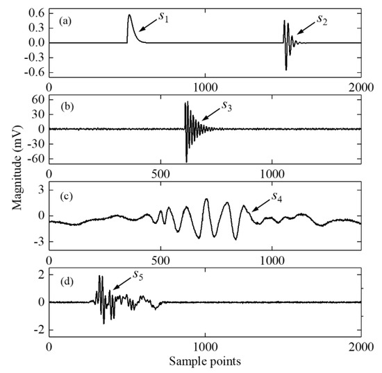
Figure 1.
Different PD signals: (a) simulated PD signals s1 (exponential decay type) and s2 (exponential oscillation type); (b) laboratory-measured PD signal s3 on a 35 kV XLPE cable joint; (c) field-detected PD signal s4 on a 10 kV XLPE cable; (d) field-detected PD signal s5 on a HV cable system.
The laboratory-measured PD signal was captured from an artificial incision defect on the insulation layer of a 35 kV XLPE cable joint. Specifically, the incision defect was made by cutting into the insulation layer along the longitudinal direction with a sharp knife. The starting point of the incision defect was at the cutoff point of the outer semiconducting layer in the cable joint. The length, width, and depth of the insulation incision defect were 100, 0.2, and 1 mm, respectively. The schematic of the experimental setup is shown in Figure 2. The voltage applied on the cable was raised gradually to 26 kV until the partial discharge is stable. Then, we recorded the PD signal. PD signals were transferred by a high-frequency current transformer (HFCT), with bandwidth and maximum sensitivity at 2.5–216 MHz and 5.83 V/A, respectively. To filter out low-frequency interference, a bandpass filter was connected between the HFCT and the digital oscilloscope. The bandwidth of the bandpass filter was 1.2–80 MHz, and the bandwidth of the sampling oscilloscope was up to 1 GHz. Moreover, the maximum sampling rate of the oscilloscope was 5 GS/s. Figure 1b shows the real PD signal s3 generated in the insulation incision defect. The sampling rate of s3 was 50 MS/s.
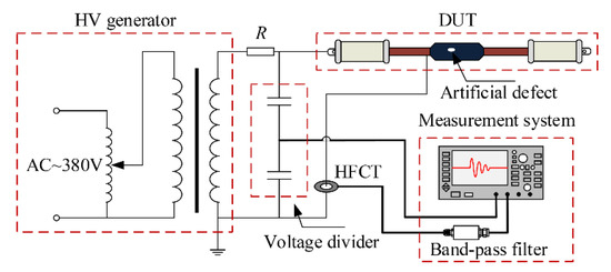
Figure 2.
Experimental setup of PD detection in the laboratory.
The field-detected PD signals s4 and s5 are shown in Figure 1c,d. s4 was measured on a 10 kV XLPE cable system with a sampling rate of 500 MS/s, and s5 was measured on a HV cable system with a sampling rate of 100 MS/s.
3. Proposed ASTSVD Method
In this section, basic principles of ASTSVD will be introduced first, including adaptive singular value selection, short-time singular value decomposition, and sliding window length selection. Then the denoising procedure is proposed, and the computational efficiency of the ASTSVD is discussed in detail.
3.1. Principle of Adaptive Singular Value Selection
In SVD-based denoising methods, after applying SVD to a signal (which is embedded in a L × K Hankel matrix before), a singular value sequence [σ1, σ2, …, σm]T (σ1 ≥ σ2 ≥ … ≥ σm = σmin (L, K)) can be acquired. Then, a method is needed to select effective singular values which will be used to reconstruct the denoised signal. Because effective singular values usually have larger values than the singular values coming from noise, and the singular value sequence is arranged in descending order, we only need to determine the number of lager singular values at the front of the sequence. For example, if we determine the number of effective singular values r = 9, singular values σ1, σ2, …, σ9 are chosen. In this paper, the minimum description length criterion (MDL) [35,36,37] is used to automatically determine r. Based on information theoretic arguments, the MDL criterion was proposed by Rissanen [38] for model selection and was used by Wax [35] for detecting the number of signals in a multichannel time-series. Rissanen’s proposal was to select the model which could minimize MDL [38]. MDL is defined as
where X is a set of observations, X = {x(1), x(2), …, x(N)}; Θ is the parameter vector of models; f(X|Θ) is a family of models (a family of probability density of Θ); is the maximum likelihood estimate of the parameter vector Θ; k is an index which can determine the number of parameters in Θ (0 ≤ k < m). In Equation (3), the first term is the log-likelihood of the maximum likelihood estimator of the parameters of the model. The second term is a bias correction term for making MDL an unbiased estimate of the mean Kulback–Liebler distance between the model density f(X|Θ) and the estimated density f(X|).
After obtaining the maximum-likelihood estimate of Θ according to Anderson [39], Wax [35] substituted the maximum likelihood estimate in the log-likelihood function of Θ and obtained log f(X|). Besides, Wax also inferred that the number of free adjusted parameters in Θ were k (2m − k + 1), where m is the total number of singular values.
According to the above-mentioned statements, the first term and the second term of Equation (3) can be obtained. Then MDL is given as
where N is the total number of signal points; σi is the singular values of the signal. Determining the number of effective singular values in this paper shares the same principle with detecting the number of signals by Wax. The number of effective singular values r is determined as the value of k ∈ {0, 1, …, m − 1}, which makes MDL minimized.
To further show how to select singular values using the MDL criterion, the MDL of simulated PD signal s1 embedded in AWGN with SNR = 30 dB was calculated. The result is shown in Figure 3. As shown in Figure 3, with the index k increasing, MDL of s1 decreased first and then increased. Therefore, there is a minimum value of MDL. r is equal to the value of k which is corresponding to the minimum value of MDL. Overestimation may happen to some other methods when they estimate the number of singular values of noise. Therefore, we also calculated the MDL of noise. The result is also shown in Figure 3. For noise, MDL is minimized when k = 0. This means that no singular value will be selected when ASTSVD is performed on noise. This experiment shows the high applicability of the MDL criterion in singular value selection.
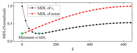
Figure 3.
MDL of PD signal s1 embedded in AWGN with SNR = 30 dB and MDL of a signal containing only noise.
Moreover, in order to show the effect of using MDL in singular value selection, we set another experiment as follows. We generated five sinusoidal signals with different frequency (1, 3.3, 5, 8.1, and 10 MHz, respectively) and the same amplitudes and phases (10 mV and 0°). Then, we mixed the sinusoidal signals together to obtain a mixed signal which contained five signal components with different frequency. ASVD [26] and MDL were used to identify r of the mixed signal, which ought to be 10. The results of singular value selection under different SNR is shown in Figure 4. The reference line consists of the correct value of r under different SNR. From Figure 4, Both ASVD and MDL performed well under high SNR. However, MDL kept relatively better performance under low SNR while ASVD overestimated the number of effective singular values. When SNR was extremely low, MDL determined r as zero.
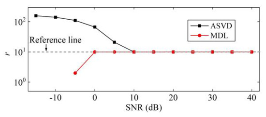
Figure 4.
Number of selected singular values of the mixed signal under different SNR.
3.2. Principle of Short-Time Singular Value Decomposition
Because of the complexity of a PD signal, even though a proper value of r is determined, features of the original PD signal still cannot be perfectly preserved. As a result, the denoised results usually exhibit waveform distortion and contain some residual noise.
To show the less satisfactory denoising result obtained by directly applying SVD to a whole PD signal, the simulated PD signal s2 was embedded in additive white Gaussian noise (AWGN) with SNR = 0 dB and denoised by SVD. The SNR is defined as Equation (6). It is worth mentioning that the number of effective singular values was chosen manually to acquire best denoised results. The normalized singular value spectrum of noisy s2 is shown in Figure 5 (30 larger singular values were selected) and the denoising result is shown in Figure 6. As shown in Figure 6, even though a proper number of effective singular values was selected, the denoised signal by SVD still contained some residual noise and exhibited waveform distortion.
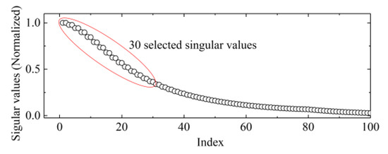
Figure 5.
Singular value spectrum of PD signal s2 embedded in AWGN (additive white Gaussian noise) with SNR = 0 dB.
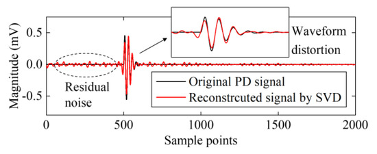
Figure 6.
SVD denoising of PD signal s2 embedded in AWGN (additive white Gaussian noise) with SNR = 0 dB.
To address this issue, we moved a sliding window point by point along the time axis of a PD signal and captured signal segments within the sliding window. The whole PD signal was divided into segments which were called signal snapshots. It is much better to perform SVD on snapshots instead of the whole signal, because it can preserve signal details better. The short-time SVD can cause less residual noise and has a better denoising effect.
3.3. Principle of Sliding Window Length Selection
The only parameter that needs to be preselected in the ASTSVD method is the sliding window length. To compare the denoising effect of ASTSVD with different sliding window lengths, two parameters, including the mean square error (MSE) [40,41] and normalized correlation coefficient (NCC) [42,43] were used to evaluate the performance of the ASTSVD. MSE and NCC are defined as
where x1 and x2 denote the original and denoised PD signals, respectively. NCC can reveal the similarity of x1 and x2, which belongs to (−1, 1). Effective denoising methods should have lower MSE and higher NCC.
ASTSVD with different sliding window lengths was applied to simulated PD signals s1 and s2 embedded in AWGN with SNR = 0 dB. Figure 7 shows the MSE and NCC of denoised results.
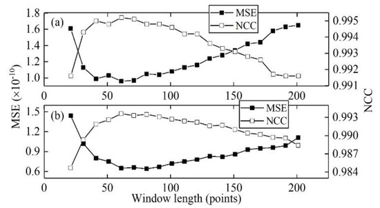
Figure 7.
MSE and NCC under different sliding window lengths: (a) The results for PD signal s1; (b) The results for PD signal s2.
The results for MSE and NCC show that ASTSVD can obtain good denoised results over a wide range of sliding window lengths. According to the results, an empirical principle of sliding window length selection in ASTSVD was summarized as follows:
Determine sliding window lengths around half of the PD’s pulse width to obtain a better denoising effect.
According to the principle above, we need to know the width of a PD pulse to determine the sliding window length. First, if we are aware of the sampling rate and general width of a PD pulse in cables (around 1 μs), we can estimate the number of sample points within the PD pulse through dividing the width of the PD pulse by the sampling rate. Then, the sliding window length can be estimated roughly according to the above-mentioned principle. Besides, time domain energy of a signal [44] and instantaneous curvature of a signal’s waveform [45] can also be used to identify boundaries of a PD pulse. In addition, ASTSVD can also locate the start points and the end points of a PD pulse by identifying the number of effective singular values r. The procedure is as follows: we move a sliding window point by point along the time axis of the PD signal. Then, we select the number of effective singular values r of each signal segment (i.e., snapshot) captured by the sliding window. Each value of r is assigned to the midpoint of the sliding window. Finally, we can obtain a singular value distribution spectrum which shows the boundaries of the PD pulse clearly. The procedure for identifying the boundary of a PD pulse by ASTSVD is shown in Figure 8. A singular value distribution spectrum is shown in Figure 9. As we know the boundaries of a PD pulse, we know its pulse width. Then, we can determine sliding window length according to the above-mentioned principle.
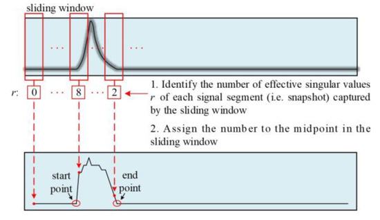
Figure 8.
The procedure for identifying the boundary of a PD pulse by ASTSVD.
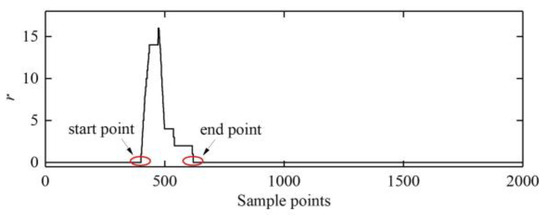
Figure 9.
A singular value distribution spectrum.
3.4. Denoising Procedure of the Proposed ASTSVD Method
The detailed denoising procedure of the proposed ASTSVD method is as follows:
- Apply a sliding window with length Tw to a noise-corrupted PD signal y = (y1, y2, y3, …, yi, …, yN). The sliding window length is an odd number in this paper.
- Use the sliding window to capture a signal snapshot yi within the sliding window. yi = (yi, yi+1, yi+2, …, yi+n-1, …, yi+Tw-1)
- Embed the snapshot yi into a L × K Hankel matrix Yi, which is defined aswhere K = Tw – L + 1; L = Tw/3 in this paper (L should be between Tw/20 [26] and Tw/2 [27]).
- Apply SVD to the Hankel matrix Yi. Then, Yi is decomposed into three matrices, aswhere U is a L × L orthogonal matrix; Σ is a diagonal matrix, Σ = diag(σ1, σ2, …, σm), m = min (L, K) and the sequence (σ1, σ2, …, σm) is sorted in descending order; V is a K × K orthogonal matrix.
- Calculate the MDL of Σ with Equation (4) and obtain the number of effective singular values r according to Equation (5).
- Reconstruct a new matrix Yi’ as
- Reconstruct a new signal snapshot yi’ by averaging the diagonal elements in the matrix Yi’:
- Move the sliding window to the next sample point (i = i +1) and repeat Step 2 to Step 8. Stop moving sliding window until i = N − (Tw − 1). Then, all new snapshots yi’ are obtained.
- Average the overlaps of snapshots yi and combine the averaged overlaps together to form a new denoised PD signal y’ (for example, in Figure 10, combine a’, b’, c’, … to form denoised signal y’).
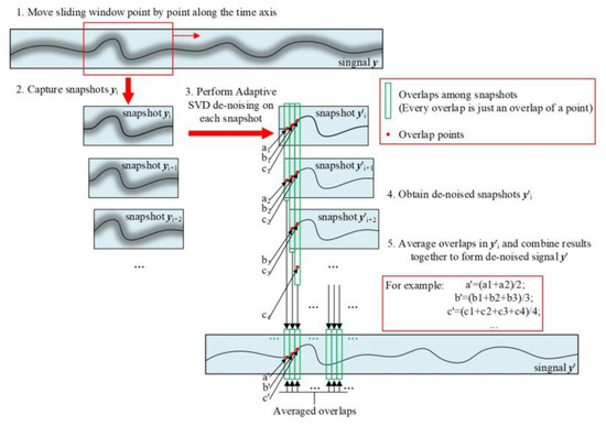 Figure 10. Steps about capturing snapshots and averaging overlaps of snapshots.
In ASTSVD, the steps about capturing snapshots and averaging overlaps of snapshots are exhibited in Figure 10. Because the sliding window moves point by point, every overlap is just an overlap of a point. Consequently, the averaged overlaps only contain one point and the denoised PD signal is formed point by point. The procedure of ASTSVD is summarized in Figure 11. In ASTSVD, it is notable that signals are processed segmentally through applying a sliding window to the PD signal. Consequently, when we deal with a PD signal with large data, the computational efficiency of ASTSVD is much higher than that of the methods which performs SVD on the whole PD signal, such as ASVD [26]. This will be further verified in the next part.
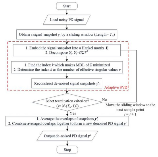
Figure 11.
The flow diagram of ASTSVD.
3.5. Computational Time Comparision of Two SVD-Based Methods
When processing PD signals with a large amount of data, ASVD [26] requires a great deal of memory and much computational time, limiting its applicability. However, by applying a sliding window, ASTSVD can reduce both the memory requirements and the computational requirements. To compare the computational time of ASVD and ASTSVD, simulated PD signals s1 of different sizes embedded in AWGN with SNR = 0 dB were denoised using ASVD and ASTSVD. The data amount of the PD signals ranged from 2000 to 10,000 sample points. Figure 12 shows that the computational time of ASVD and ASTSVD varies with the size of PD signals. ASTSVD consumes much less computation time than ASVD when processing large amounts of data. Even when the sliding window lengths increase, the computational time of ASTSVD is still much less than that of ASVD.
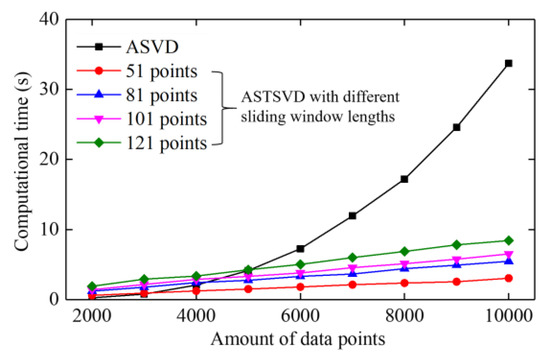
Figure 12.
Computational time of ASVD and ASTSVD versus the data amount of PD signals.
4. Denoising Effect of ASTSVD
To verify the actual effect and confirm the superiority of ASTSVD, three methods (a DWT-based method, ASVD, and ASTSVD) were applied to different PD signals (including simulated, laboratory-measured, and field-detected PD signals with low SNR and simulated PD signals with high SNR).
4.1. Simulated PD Signals
First, the denoising effect of ASTSVD was investigated on simulated PD signals. The two simulated PD signals s1 and s2 were embedded in additive white Gaussian noise (AWGN) with SNR = 0 dB. Subsequently, the denoising procedures were performed for the DWT-based denoising method (db8 wavelet, 6 level decomposition, hard thresholding) [4], ASVD [26], and ASTSVD (Tw = 101). The denoised results are respectively shown in Figure 13 and Figure 14.
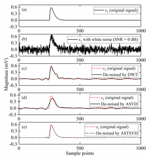
Figure 13.
Denoised results for s1: (a) The original PD signal; (b) The signal embedded in AWGN with SNR = 0 dB; (c–e) Denoised signals by the DWT-based method, ASVD, and ASTSVD.
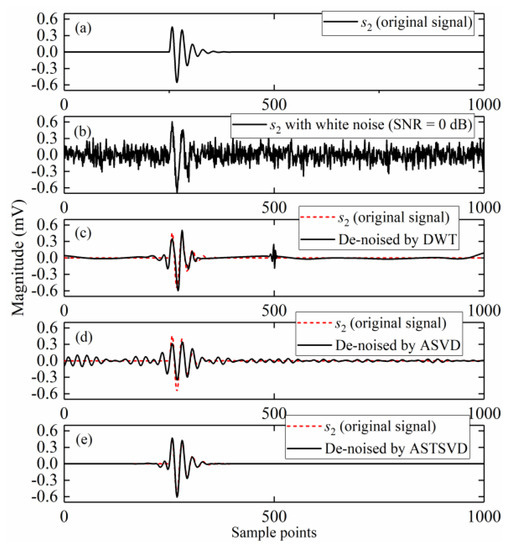
Figure 14.
Denoised results for s2: (a) The original PD signal; (b) The signal embedded in AWGN with SNR = 0 dB; (c–e) Denoised signals by the DWT-based method, ASVD, and ASTSVD.
As shown in Figure 13 and Figure 14, compared with the results of the DWT-based method and ASVD, the ASTSVD denoising results are more approximate to the original PD signals. Because s2 is oscillated, some oscillation occurred in the ASVD result, as depicted in Figure 14d. Table 1 demonstrates the MSE, NCC, and SNR of the two PD signals which were denoised by using different denoising methods (related calculations were repeated 100 times, and the results were averaged). As shown, ASTSVD is much better than the other two methods.

Table 1.
MSE, NCC, and SNR of denoised PD signals s1 and s2.
4.2. Laboratory-Measured PD Signal
To verify the effect of ASTSVD on practical PD signals, the laboratory-measured PD signals was denoised. Then, wavelet shrinkage with db8 wavelet and soft thresholding was applied to it to obtain the original PD signal of s3 [4]. Figure 15 shows the original PD signal of s3 and its corresponding noisy PD signal embedded in AWGN with SNR = 0 dB, together with denoised results from the three denoising methods (the DWT-based method, ASVD, and ASTSVD). db8 wavelet, 6 levels of decomposition, and hard thresholding were used in the DWT-based method. The length of the sliding window Tw was 101 points in ASTSVD according to the principle mentioned in Section 3.3.
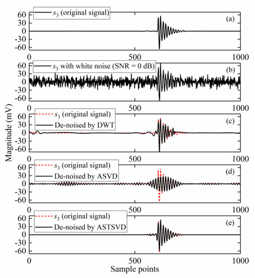
Figure 15.
Denoised results for s3: (a) The original PD signal; (b) The signal embedded in AWGN with SNR = 0 dB; (c–e) Denoised signals by the DWT-based method, ASVD, and ASTSVD.
As shown in Figure 15, ASTSVD performs relatively better in the denoising of s3 whereas ASVD loses many basic features of the original signal and generates some oscillations in the denoised signal. ASTSVD is also optimal according to MSE, NCC, and SNR, as shown in Table 2.
Table 2.
MSE, NCC, and SNR of denoised PD signals s3.
4.3. Field-Detected PD Signals
Compared with PD signals measured in the laboratory, field-detected PD signals often have irregular pulse waveforms. Hence, using field-detected PD signals to verify the denoising effect of ASTSVD is necessary. As mentioned in Section 2, s4 and s5 are field-detected PD signals with different waveforms. Wavelet shrinkage with db8 wavelet and soft thresholding was used to obtain the original PD signals of s4 and s5 [4]. Afterward, real noise collected in the field was added to the original signals of s4 and s5 with SNR = 0 dB. Three denoising methods were applied to the noisy PD signals. db8 wavelet, six levels of decomposition, and hard thresholding were used in the DWT-based method. The lengths of the sliding windows we used in ASTSVD were 101 points and 121 points for s4 and s5, respectively.
The denoised results of s4 and s5 are shown in Figure 16 and Figure 17, respectively. Table 3 shows the evaluation results based on MSE, NCC, and SNR. Although, the denoised results of s4 by using the DWT-based method and ASTSVD seem close in Figure 16, the MSE, NCC, and SNR results of ASTSVD are still better than the results of the DWT-based method.
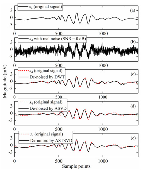
Figure 16.
Denoised results for s4: (a) The original PD signal; (b) The signal embedded in AWGN with SNR = 0 dB; (c–e) Denoised signals by the DWT-based method, ASVD, and ASTSVD.
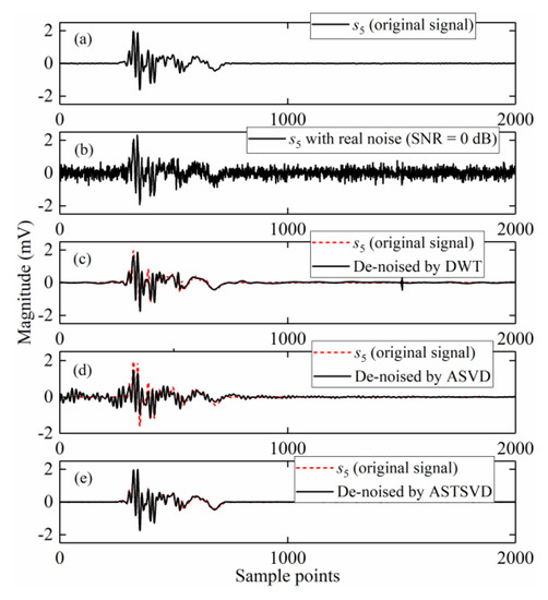
Figure 17.
Denoised results for s5: (a) The original PD signal; (b) The signal embedded in AWGN with SNR = 0 dB; (c–e) Denoised signals by the DWT-based method, ASVD, and ASTSVD.
Table 3.
MSE, NCC, and SNR of denoised PD signals s4 and s5.
4.4. Performance of ASTSVD Under High SNR
When some denoising methods are applied to a PD signals with high SNR, waveform distortion of the PD pulse may occur in the denoised results. To show the performance of ASTSVD under high SNR, simulated PD signal s1 embedded in AWGN with SNR = 30 dB was filtered by ASTSVD and ASVD.
Figure 18 shows the denoised PD signals by ASTSVD and ASVD. The denoised results indicate that ASVD may cause waveform distortion and generated some oscillations, even though a proper value of r was selected automatically (21 singular values were selected by ASVD in this experiment). However, the ASTSVD with a sliding window (Tw = 101) reconstructed the original PD signal without waveform distortion even under high SNR.
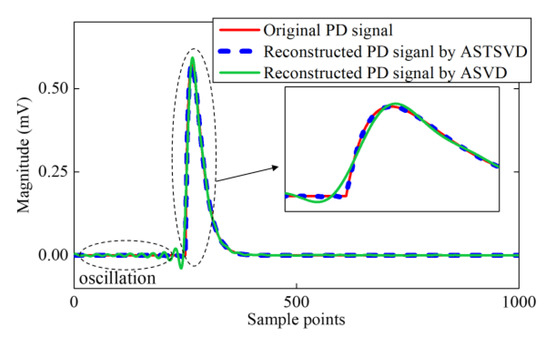
Figure 18.
Results for PD signal s1 reconstruction by ASTSVD and ASVD under high SNR.
5. Conclusions
This paper proposed a denoising method of PD signals called ASTSVD based on singular value decomposition. To achieve better denoising effect and higher computational efficiency, a sliding window is applied to the PD signal under processing. Length of the sliding window is suggested to be about half of the PD’s pulse width. While the sliding window moves along the time axis of the PD signal, snapshots of the PD signal are captured. Adaptive SVD is applied to each snapshot respectively instead of being applied to a whole PD signals for once, resulting in less residual noise and waveform distortion in the denoised signal. Besides, the minimum description length (MDL) criterion is proved to be effective in effective singular value selection. The denoised results showed the better performance of ASTSVD compared to the performance of ASVD and a DWT-based denoising method.
However, for ASTSVD, there are still some limitations. Determination of the optimal sliding window length is still unsolved. Besides, the computational time of ASTSVD is still longer than that of DWT-based methods. In addition, ASTSVD is only used in the denoising of white noise in this paper. Other applications of ASTSVD need to be developed, such as denoising of period narrowband interference. ASTSVD may also be used in image processing and seismic signal denoising in the future.
Author Contributions
Conceptualization, K.Z. and M.X.; Data curation, Y.H.; Formal analysis, M.L.; Funding acquisition, K.Z.; Investigation, Y.L.; Methodology, M.L.; Project administration, K.Z.; Resources, Y.H.; Software, M.X.; Supervision, K.Z.; Validation, M.L., Y.L., and Y.H.; Visualization, M.L.; Writing—original draft, M.L.; Writing—review and editing, M.L. and Y.L.
Funding
This research was funded by the National Natural Science Foundation of China, grant number 51477106 and 51877142 and the Fundamental Research Funds for Central Universities, grant number YJ201882.
Conflicts of Interest
The authors declare no conflict of interest.
References
- Tian, Y.; Lewin, P.L.; Davies, A.E. Coparison of on-line partial discharge detection methods for HV cable joints. IEEE Trans. Dielectr. Electr. Insul. 2002, 9, 604–615. [Google Scholar] [CrossRef]
- Chan, K.-P.; Fu, W.-C. Efficient time series matching by wavelet. In Proceedings of the 15th International Conference on Data Engineering, Sydney, NSW, Australia, 23–26 March 1999. [Google Scholar]
- Ma, X.; Zhou, C.; Kemp, I.J. Automated wavelet selection and thresholding for PD detection. IEEE Electr. Insul. Mag. 2002, 18, 37–45. [Google Scholar] [CrossRef]
- Li, J.; Jiang, T.; Grzybowski, S.; Cheng, C. Scale dependent wavelet selection for denoising of partial discharge detection. IEEE Trans. Dielectr. Electr. Insul. 2010, 17, 1705–1714. [Google Scholar] [CrossRef]
- Cunha, C.; Carvalho, A.; Petraglia, M.; Limaa, A. A new wavelet selection method for partial discharge denoising. Electr. Pow. Syst. Res. 2015, 125, 184–195. [Google Scholar] [CrossRef]
- Hussein, R.; Shaban, K.; El-Hag, A. Wavelet transform with histogram-based threshold estimation for online partial discharge signal denoising. IEEE Trans. Instrum. Meas. 2015, 64, 3601–3614. [Google Scholar] [CrossRef]
- Huang, N.; Shen, Z.; Long, S.; Wu, M.; Shih, H.; Zheng, Q.; Yen, N.; Tung, C.; Liu, H. The empirical mode decomposition and the Hilbert spectrum for nonlinear and non-stationary time series analysis. Proc. R. Soc. A– Math. Phy. Eng. Sci. 1998, 454, 903–995. [Google Scholar] [CrossRef]
- Tang, Y.; Tai, C.; Su, C.; Chen, C.; Chen, J. A correlated empirical mode decomposition method for partial discharge signal denoising. Meas. Sci. Technol. 2010, 21, 1–11. [Google Scholar] [CrossRef]
- Pan, L.; Liu, K.; Jiang, J.; Ma, C.; Tian, M.; Liu, T. A denoising algorithm based on EEMD in Raman-based distributed temperature sensor. IEEE Sens. J. 2017, 17, 134–138. [Google Scholar] [CrossRef]
- Lin, C.; Wang, J.; Cheng, Z. Fast ensemble empirical mode decomposition for speech-like signal analysis using shaped noise addition. In Proceedings of the IEEE International Conference on Interaction Sciences (ICIS), Busan, Korea, 16–18 August 2011. [Google Scholar]
- Chan, J.; Ma, H.; Saha, T.; Ekanayake, C. Self-adaptive partial discharge signal denoising based on ensemble empirical mode decomposition and automatic morphological thresholding. IEEE Trans. Dielectr. Electr. Insul. 2014, 21, 294–303. [Google Scholar] [CrossRef]
- Jin, T.; Li, Q.; Mohamed, M. A novel adaptive EEMD method for switchgear partial discharge signal denoising. IEEE Access 2019, 7, 58139–58147. [Google Scholar] [CrossRef]
- Abdel-Galil, T.; El-Hag, A.; Gaouda, A.; Salama, M.; Bartnikas, R. Denoising of partial discharge signal using eigen-decomposition technique. IEEE Trans. Dielectr. Electr. Insul. 2008, 15, 1657–1662. [Google Scholar] [CrossRef]
- Hu, L.; Ma, H.; Zhang, H.; Zhao, W. Improved singular value decomposition-based denoising algorithm in digital receiver front-end. IET Commun. 2017, 11, 2049–2057. [Google Scholar] [CrossRef]
- Viljoen, H.; Nel, D.G. Common singular spectrum analysis of several time series. J. Stat. Plan. Inference 2010, 140, 260–267. [Google Scholar] [CrossRef]
- Ghanati, R.; Hafizi, M.K.; Mahmoudvand, R.; Fallahsafari, M. Filtering and parameter estimation of surface-NMR data using singular spectrum analysis. J. Appl. Geophys. 2016, 130, 118–130. [Google Scholar] [CrossRef]
- Wang, S.; Meng, X.; Yin, Y.; Wang, Y.; Yang, X.; Zhang, X.; Peng, X.; He, W.; Dong, G.; Chen, H. Optical image watermarking based on singular value decomposition ghost imaging and lifting wavelet transform. Opt. Laser. Eng. 2019, 114, 76–82. [Google Scholar] [CrossRef]
- Yao, L.; Yuan, C.; Qiang, J.; Feng, S.; Nie, S. Asymmetric color image encryption based on singular value decomposition. Opt. Laser. Eng. 2017, 89, 80–87. [Google Scholar] [CrossRef]
- Zhang, X.; Peng, J.; Xu, M.; Yang, W.; Zhang, Z.; Guo, H.; Chen, W.; Feng, Q.; Wu, X.; Feng, Y. Denoise diffusion-weighted images using higher-order singular value decomposition. NeuroImage 2017, 156, 128–145. [Google Scholar] [CrossRef]
- Rekapalli, R.; Tiwari, R.K.; Sen, M.K.; Vedanti, N. 3D seismic data denoising and reconstruction using multichannel time slice singular spectrum analysis. J. Appl. Geophys. 2017, 140, 145–153. [Google Scholar] [CrossRef]
- Iqbal, N.; Zerguine, A.; Kaka, S.L.; Al-Shuhail, A. Automated SVD filtering of time-frequency distribution for enhancing the SNR of microseismic/microquake events. J. Geophys. Eng. 2016, 13, 964–973. [Google Scholar] [CrossRef]
- Yi, C.; Lv, Y.; Dang, Z.; Xiao, H.; Yu, X. Quaternion singular spectrum analysis using convex optimization and its application to fault diagnosis of rolling bearing. Measurement 2017, 103, 321–332. [Google Scholar] [CrossRef]
- Li, H.; Liu, T.; Wu, X.; Chen, Q. Research on bearing fault feature extraction based on singular value decomposition and optimized frequency band entropy. Mech. Syst. Signal Proc. 2019, 118, 477–502. [Google Scholar] [CrossRef]
- Hassani, H.; Ghodsi, Z. A glance at the applications of singular spectrum analysis in gene expression data. Biomol. Detect. Quantif. 2015, 4, 17–21. [Google Scholar] [CrossRef] [PubMed]
- Yang, B.; Dong, Y.; Yu, C.; Hou, Z. Singular spectrum analysis window length selection in processing capacitive captured biopotential signals. IEEE Sens. J. 2016, 6, 7183–7193. [Google Scholar] [CrossRef]
- Ashtiani, M.B.; Shahrtash, S.M. Partial discharge denoising employing adaptive singular value decomposition. IEEE Trans. Dielect. Electr. Insul. 2014, 21, 775–782. [Google Scholar] [CrossRef]
- Wang, R.; Ma, H.; Liu, G.; Zuo, D. Selection of window length for singular spectrum analysis. J. Frankl. Inst. 2015, 352, 1541–1560. [Google Scholar] [CrossRef]
- Elsner, J.B.; Tsonis, A.A. Singular Spectrum Analysis: A New Tool in Time Series Analysis; Plenum: New York, NY, USA, 1996. [Google Scholar]
- Alharbi, N.; Hassani, H. A new approach for selecting the number of the eigenvalues in singular spectrum analysis. J. Frankl. Inst. 2016, 353, 1–16. [Google Scholar] [CrossRef]
- Zhou, Y.; Zhu, Z. A hybrid method for noise suppression using variational mode decomposition and singular spectrum analysis. J. Appl. Geophys. 2019, 161, 105–115. [Google Scholar] [CrossRef]
- Konstantinides, K.; Natarajan, B.; Yovanof, G.S. Noise estimation and filtering using block-based singular value decomposition. IEEE Trans. Image Process 1997, 6, 479–483. [Google Scholar] [CrossRef]
- Shih, Y.-T.; Chien, C.-S.; Chuang, C.-Y. An adaptive parameterized block-based singular value decomposition for image denoising and compression. Appl. Math. Comput. 2012, 218, 10370–10385. [Google Scholar]
- Leles, M.C.R.; Sansão, J.P.H.; Mozelli, L.A.; Guimarães, H.N. Improving reconstruction of time-series based in singular spectrum analysis: A segmentation approach. Digit. Signal Process. 2018, 77, 63–76. [Google Scholar] [CrossRef]
- Yiou, P.; Sornette, D.; Ghil, M. Data-adaptive wavelets and multi-scale singular-spectrum analysis. Phisica D 2000, 142, 254–290. [Google Scholar] [CrossRef]
- Wax, M.; Kailath, T. Detection of signals by information theoretic criteria. IEEE Trans. Signal Process. 1985, 6, 387–392. [Google Scholar] [CrossRef]
- Zarowski, C.J. The MDL criterion for rank determination via effective singular values. IEEE Trans. Signal Process. 1998, 46, 1741–1744. [Google Scholar] [CrossRef]
- Yang, X.; Li, S.; Hu, X.; Zeng, T. Improved MDL method for estimation of source number at subarray level. Electron. Lett. 2016, 52, 85–86. [Google Scholar] [CrossRef]
- Rissanen, J. Modeling by shortest data description. Automatica 1978, 14, 465–471. [Google Scholar] [CrossRef]
- Anderson, T.W. Asymptotic theory for principal component analysis. Ann. J. Math. Stat. 1963, 34, 122–148. [Google Scholar] [CrossRef]
- Jain, S.; Bajaj, V.; Kumar, A. Effective denoising of ECG by optimized adaptive thresholding on noisy mode. IET Sci. Meas. Technol. 2018, 12, 640–644. [Google Scholar] [CrossRef]
- Le Montagner, Y.; Angelini, E.D.; Olivo-Marin, J. An unbiased Risk estimator for image denoising in the presence of mixed Poisson–Gaussian noise. IEEE Trans. Image Process. 2014, 23, 1255–1268. [Google Scholar] [CrossRef]
- Zhang, X.; Zhou, J.; Li, N.; Wang, Y. Suppression of UHF partial discharge signals buried in white-noise interference based on block thresholding spatial correlation combinative denoising method. IET Gener. Transm. Dis. 2012, 6, 353–362. [Google Scholar] [CrossRef]
- Zhou, M.; Xia, H.; Zhong, H.; Zhang, J.; Gao, F. A noise reduction method for photoacoustic imaging in vivo based on EMD and conditional mutual information. IEEE Photon. J. 2019, 11, 1–10. [Google Scholar] [CrossRef]
- Gerber, A.; Studer, R.M.; de Figueiredo, R.J.P.; Moschytz, G.S. A new framework and computer program for quantitative EMG signal analysis. IEEE Trans. Biomed. Eng. 1984, BME-31, 857–863. [Google Scholar] [CrossRef] [PubMed]
- Jager, F.; Koren, I.; Gyergyek, L. Multiresolution representation and analysis of ECG waveforms. In Proceedings of the Computers in Cardiology, Chicago, IL, USA, 23–26 September 1990. [Google Scholar]
© 2019 by the authors. Licensee MDPI, Basel, Switzerland. This article is an open access article distributed under the terms and conditions of the Creative Commons Attribution (CC BY) license (http://creativecommons.org/licenses/by/4.0/).