Comparative Analysis of Identification Methods for Mechanical Dynamics of Large-Scale Wind Turbine


Abstract
:1. Introduction
- Structural identifiability analysis of the two-mass model under general closed-loop control conditions across the whole wind speed range is presented and is useful to judge feasibility of parameter identification in the closed-loop.
- Influence of identified data to identification performance is discussed based on mutual information analysis of identified variables and is helpful to select great identified datasets.
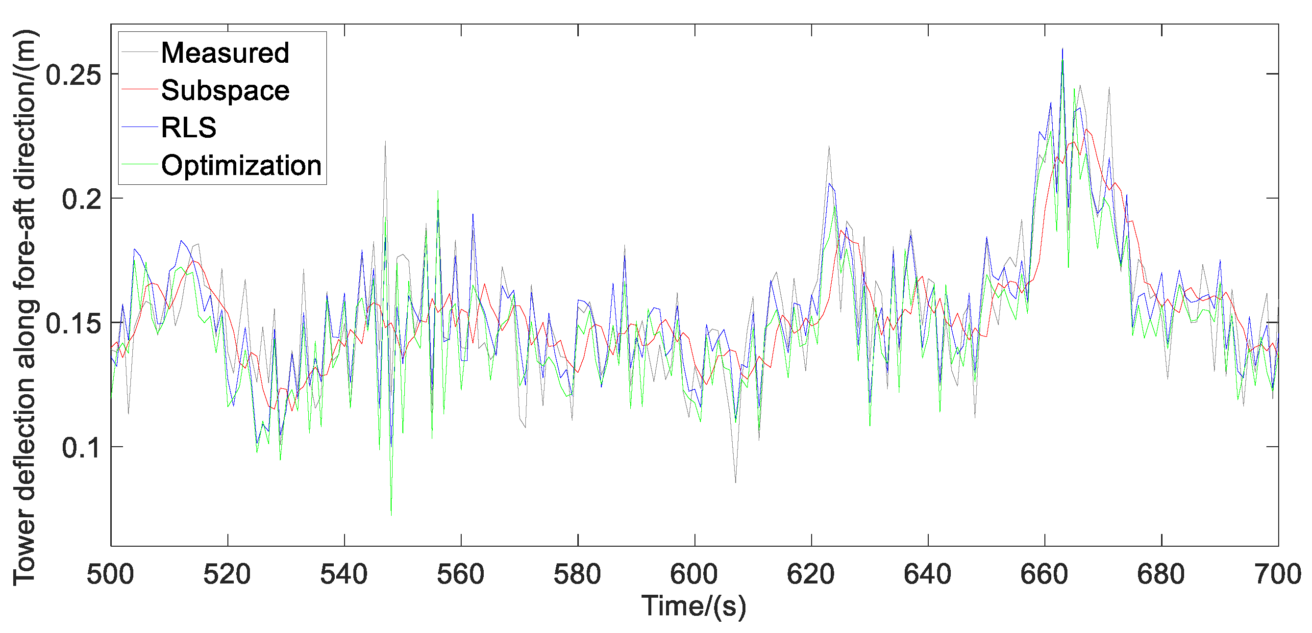
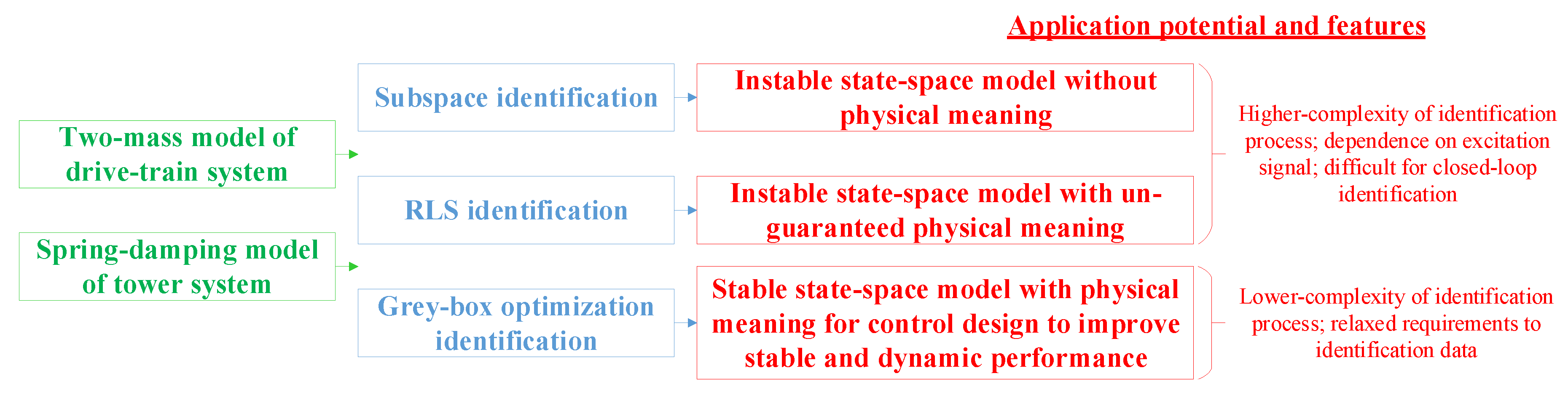
- Grey-box identifications for mechanical dynamics of a wind turbine, including the two-mass model of drive-train and the two-order damping model of tower-top, are studied where subspace identification, RLS and optimal identification are compared under wind scenarios with different turbulence intensities.
- Identification performances and features of different methods are analyzed from views of control design, providing guiding opinions for further improvement.
2. Basic Knowledge of The Modern VSVP Wind Turbine
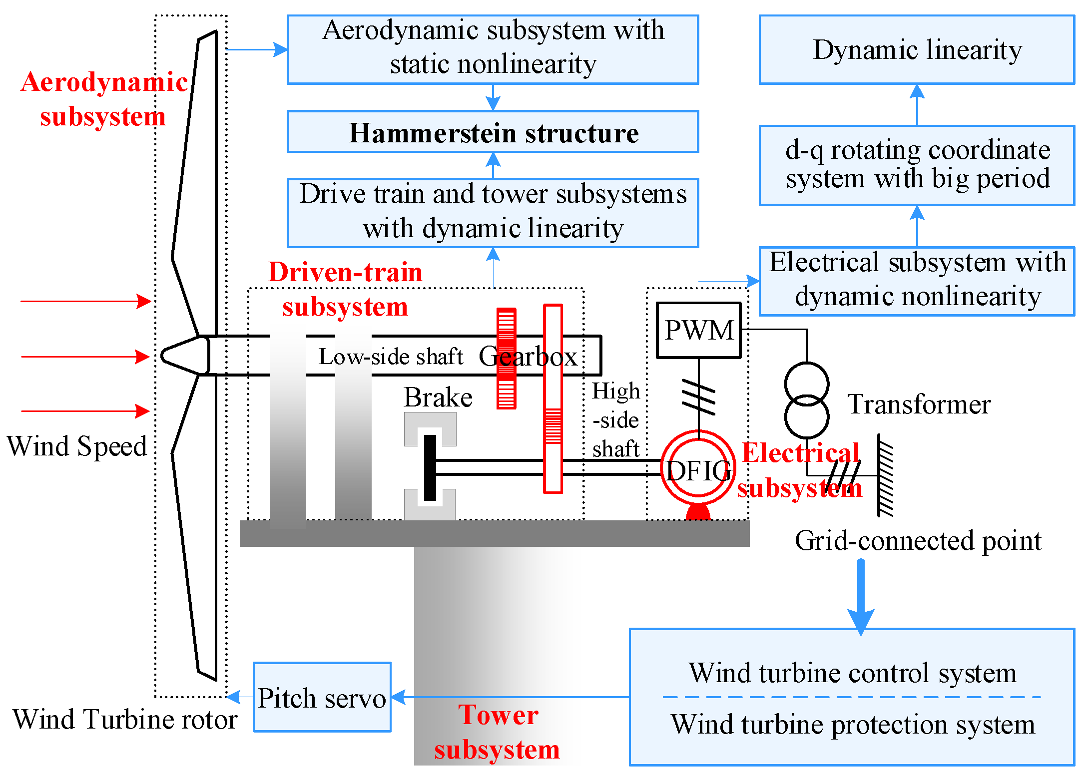
2.1. Rationality of Hammerstein Structure
2.2. Selected Subsystem Models
2.2.1. Aerodynamic Subsystem
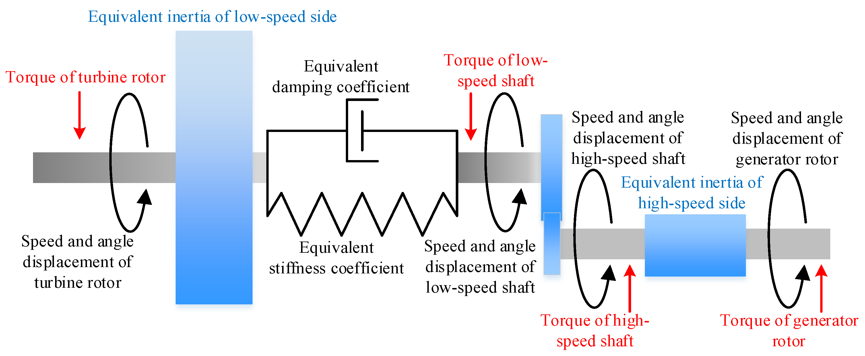
2.2.2. Drive-Train Subsystem
2.2.3. Tower Subsystem
3. Identifiability Analysis under Closed-Loop Condition
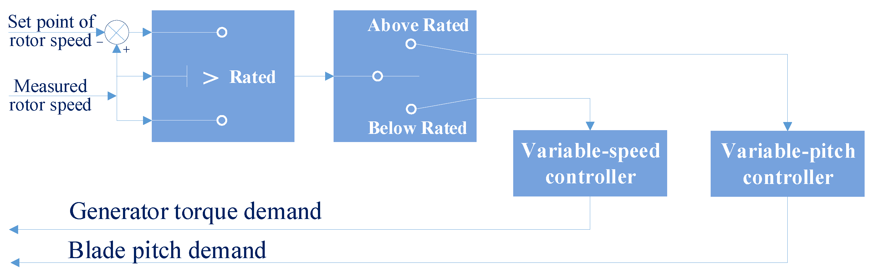
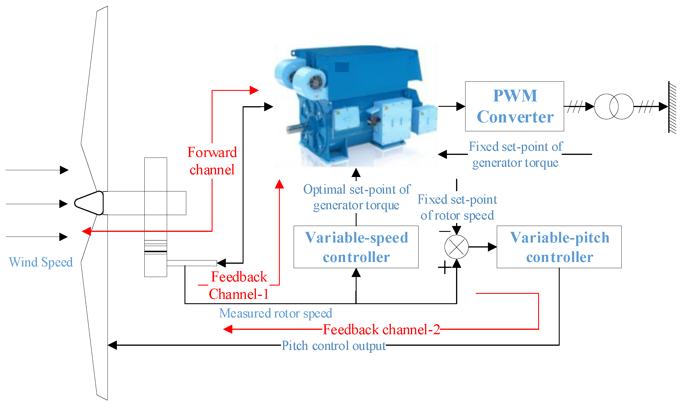
3.1. Control Strategy of Modern VSVP Wind Turbine
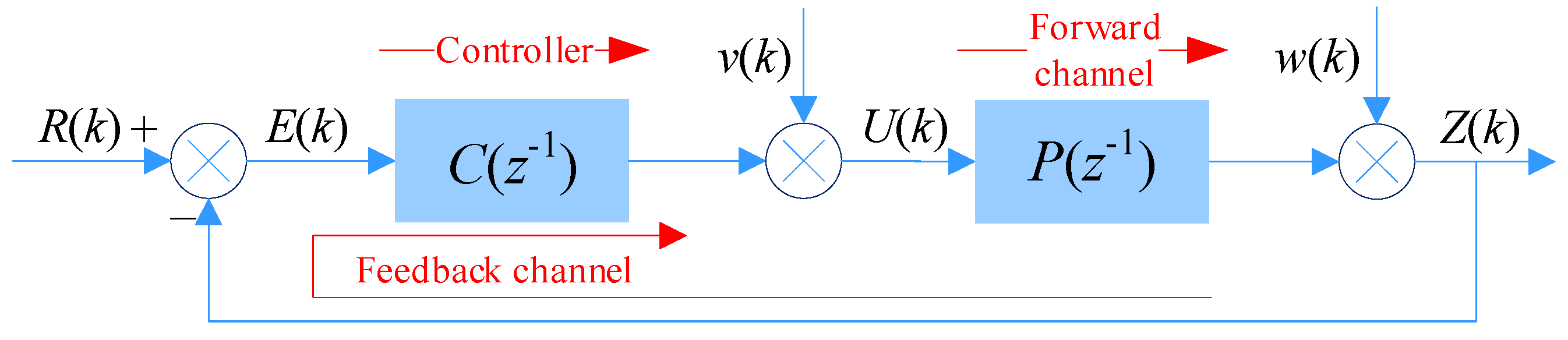
3.2. Structural Identifiability Analysis of Closed-Loop Control System
- If feedback channel is linear and invariant while no disturbance signal exists and set-point is constant, the identifiable condition is that cancellation between zeros and poles of closed-loop transfer function does not happen, caused by model structure of the feedback channel. Meanwhile, np ≥ nb, nq ≥ na−dt where np and nq are denominator and numerator order of C(z−1); na and nb are those of P(z−1); dt is time delay between output and input of the forward channel.
- If continuous excitation signal with enough order exists on the feedback channel and is irrelevant with the noise on the forward channel, a closed-loop system is structurally identifiable.
- If controller is time-varying or nonlinear, a closed-loop is structurally identifiable.
- If the controller switches among several regulation laws, closed-loop is structurally identifiable. For a multi-variable control system, it requires l ≥ 1 + r/m, where l is number of feedback controllers; r and m are input and output dimensions of closed-loop.
3.3. Correlation Analysis of Identified Data
4. Execution of Identification
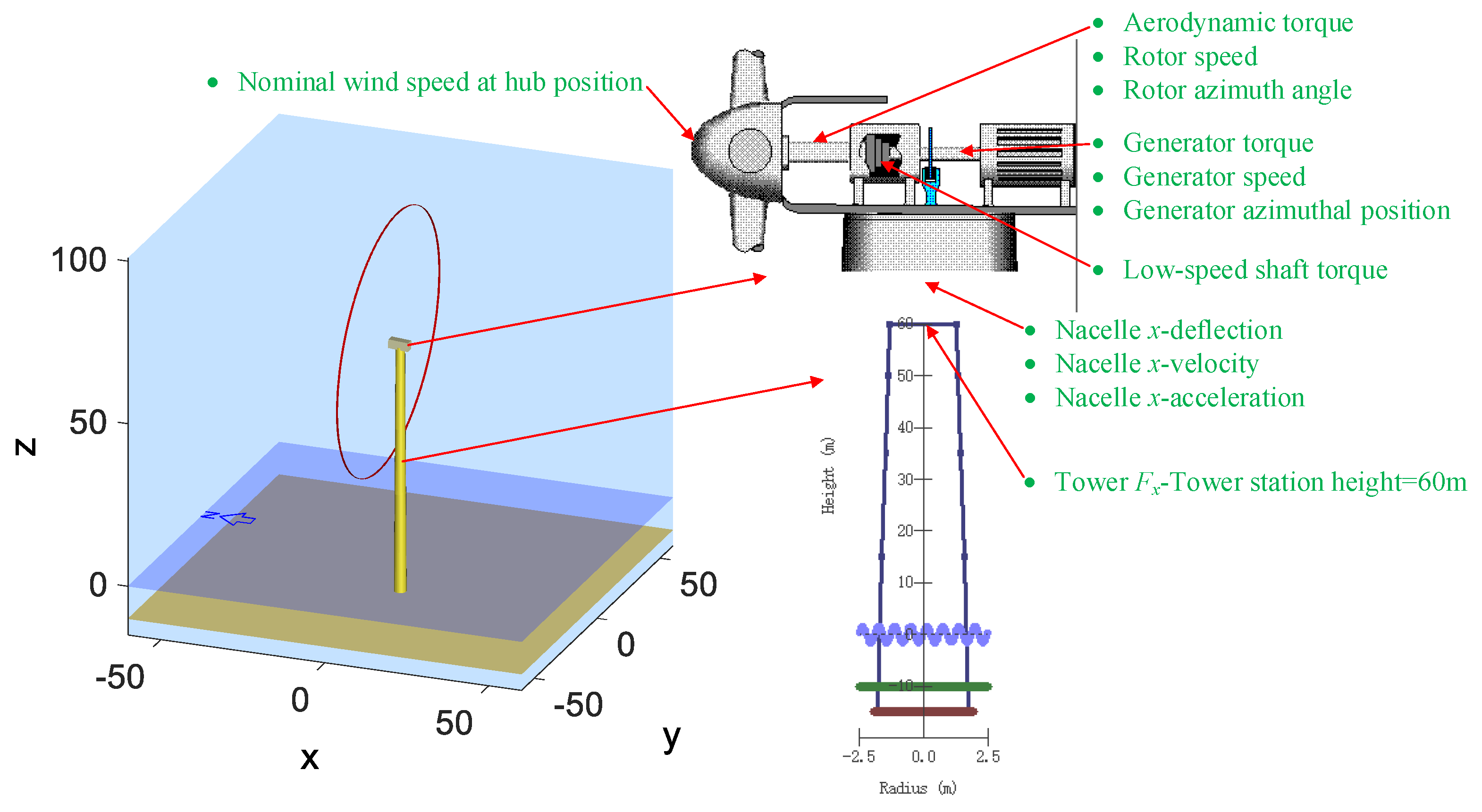
4.1. Data Acquisition and Preprocessing
4.2. Optimization Criterion
4.3. Brief Introduction of Identification Algorithms
4.3.1. Subspace Identification
4.3.2. Grey-Box Parameter Identification via Recursive Least Squares Algorithm
4.3.3. Grey-Box Parameter Identification via Optimization Algorithm
- Step 1:
- Set sampling period, acquire data samples and execute data preprocessing.
- Step 2:
- Set weighting coefficients of optimization criterion.
- Step 3:
- Estimate and set initial domains of identified parameters.
- Step 4:
- Identify unknown parameters using optimization algorithms.
- Step 5:
- Test identified dynamics of each input–output channel. If huge deviation happens, adjust certain steps and repeat Step 4. If required performance is fulfilled, the procedure is over.
5. Simulation
5.1. Parameters Setting
5.2. Scenarios Setting and Simulation
6. Conclusions
Author Contributions
Funding
Conflicts of Interest
Abbreviations
| AEC | aero-elastic code |
| ANN | artificial neural network |
| ARMAX | auto-regressive moving average |
| ARX | auto-regressive |
| BEM | blade element momentum |
| BJ | Box-Jenkins |
| CVA | canonical variate analysis |
| DFIG | double-fed induction generator |
| LCOE | levelized cost of energy |
| LIDAR | light detection and range |
| LS | least square |
| MI | mutual information |
| MOESP | multivariable output error state space |
| MSE | mean squared error |
| OE | output-error |
| OTC | optimal torque control |
| PBSIDopt | prediction-based subspace identification |
| PEM | prediction-error method |
| PI | proportional-integral |
| PRBS | pseudo-random binary excitation signals |
| PSO | particle swarm optimization |
| PWM | pulse width modulation |
| RLS | recursive least square |
| SSARX | space state autoregressive exogenous |
| SVM | support vector machine |
| VSVP | variable-speed variable-pitch |
Appendix A


| Distance from root (m) | 0 | 3.44444 | 5.74074 | 9.18519 | 16.0741 | 26.4074 | 35.5926 | 38.75 |
| Centre of mass (%) | 50 | 38 | 29 | 29 | 29 | 29 | 29 | 29 |
| Mass per unit length (kg/m) | 1084.77 | 277.356 | 234.212 | 209.558 | 172.577 | 103.546 | 55.4713 | 24.6539 |
| Flapwise stiffness (Nm/rad) | 7.472 × 10⁹ | 1.408 × 10⁹ | 8.341 × 10⁸ | 5.561 × 10⁸ | 2.058 × 10⁸ | 2.954 × 10⁷ | 2.259 × 10⁶ | 3127.98 |
| Edgewise stiffness (Nm/rad) | 7.472 × 10⁹ | 2.085 × 10⁹ | 1.425 × 10⁹ | 1.286 × 10⁹ | 5.648 × 10⁸ | 1.216 × 10⁸ | 2.433 × 10⁷ | 8167.51 |
| Angle of incidence (deg) | −180 | −141.27 | −100.65 | −19 | 0 | 21.61 | 115.85 | 150.54 | 180 |
| Lift coefficient | −0.088 | 0.716 | 0.094 | −0.354 | 0.449 | 0.806 | −0.539 | −0.674 | −0.088 |
| Drag coefficient | 0.036 | 0.772 | 1.167 | 0.191 | 0.007 | 0.288 | 1.094 | 0.466 | 0.036 |
| Pitch coefficient | −0.041 | 0.362 | 0.313 | 0.042 | −0.079 | −0.097 | −0.363 | −0.301 | −0.041 |
References
- Kumar, Y.; Ringenberg, J.; Depuru, S.S.; Devabhaktuni, V.K.; Lee, J.W.; Nikolaidis, E.; Andersen, B.; Afjeh, A. Wind energy: Trends and enabling technologies. Renew. Sust. Energ. Rev. 2016, 53, 209–224. [Google Scholar] [CrossRef]
- Eduardo, J.N.M.; Alex, M.A.; da Silva, N.; Nadege, S.B. A review on wind turbine control and its associated methods. J. Clean. Prod. 2018, 174, 945–953. [Google Scholar] [CrossRef]
- Njiri, J.G.; Dirk, S. State-of-the-art in wind turbine control: Trends and challenges. Renew. Sust. Energ. Rev. 2016, 60, 377–393. [Google Scholar] [CrossRef]
- Yuan, Y.; Tang, J. On advanced control methods toward power capture and load mitigation in wind turbines. Engineering 2017, 3, 494–503. [Google Scholar] [CrossRef]
- Menezes, E.J.N.; Araújo, A.M.; Rohatgi, J.S.; Foyo, P.M.G. Active load control of large wind turbines using state-space methods and disturbance accommodating control. Energy 2018, 150, 310–319. [Google Scholar] [CrossRef]
- Gao, R.; Gao, Z. Pitch control for wind turbine systems using optimization, estimation and compensation. Renew. Energy 2016, 91, 501–515. [Google Scholar] [CrossRef]
- Kelouwani, S.; Agbossou, K. Nonlinear model identification of wind turbine with a neural network. IEEE Trans. Energy Conver. 2004, 19, 607–612. [Google Scholar] [CrossRef]
- Sun, P.; Li, J.; Wang, C.; Lei, X. A generalized model for wind turbine anomaly identification based on SCADA data. Appl. Energ. 2016, 168, 550–567. [Google Scholar] [CrossRef] [Green Version]
- Prajapat, G.P.; Senroy, N.; Kar, I.N. Wind turbine structural modeling consideration for dynamic studies of DFIG based system. IEEE T Sustain. Energ. 2017, 8, 1463–1472. [Google Scholar] [CrossRef]
- Wang, L.; Zhang, Z.; Long, H.; Xu, X.; Liu, R. Wind turbine gearbox failure identification with deep neural networks. IEEE T. Ind. Inf. 2017, 13, 1360–1368. [Google Scholar] [CrossRef]
- Carcangiu, C.E.; Balaguer, I.F.; Kanev, S.; Rossetti, M. Closed-loop system identification of Alstom 3MW wind turbine. In Conference Proceedings of the Society for Experimental Mechanics Series; Springer: New York, USA, 2011; Volume 4, pp. 121–128. [Google Scholar]
- Iribas, M.; Landau, I.D. Identification in closed loop operation of models for collective pitch robust controller design. Wind Energy 2013, 16, 383–399. [Google Scholar] [CrossRef]
- Ye, H.Y. Control Technology of Wind Turbines, 3rd ed.; China Machine Press: Beijing, China, 2015; ISBN 9787111500179. [Google Scholar]
- Van der Veen, G.J.; van Wingerden, J.W.; Fleming, P.A.; Scholbrock, A.K.; Verhaegen, M. Global data-driven modeling of wind turbines in the presence of turbulence. Control Eng. Pract. 2013, 21, 441–454. [Google Scholar] [CrossRef]
- Loh, C.H.; Loh, K.J.; Yang, Y.S.; Hsiung, W.Y.; Huang, Y.T. Vibration-based system identification of wind turbine system. Struct. Control Hlth. 2016, 24, 1–19. [Google Scholar] [CrossRef]
- Aarden, P. System Identification of the 2B6 Wind Turbine-a Regularized PBSIDopt Approach. Master’s Thesis, Delft University of Technology, Delft, The Netherlands, 2017. [Google Scholar]
- Jonkman, J.M.; Buhl, M.L., Jr. FAST User’s Guide; Technical Report: NREL/TP-500-38230; National Renewable Energy Laboratory: Golden, CA, USA, 2005.
- Hsu, M.C.; Akkerman, I.; Bazilevs, Y. Finite element simulation of wind turbine aerodynamics: Validation study using NREL Phase VI experiment. Wind Energy 2014, 17, 461–481. [Google Scholar] [CrossRef]
- DNV GL-Energy. Theory Manual Bladed; Garrad Hassan & Partners Ltd: Bristol, UK, 2014. [Google Scholar]
- Bianchi, F.D.; De Battista, H.; Mantz, R.J. Wind Turbine Control Systems: Principles, Modelling and Gain Scheduling Design; Springer: London, UK, 2007; ISBN 1-84628-492-9. [Google Scholar]
- Munteanu, I.; Bratcu, A.I.; Cutululis, N.A.; Ceangă, E. Optimal Control of Wind Energy Systems-Towards Global Approach; Springer: London, UK; ISBN 978-1-84800-079-7.
- Ebadollahi, S.; Saki, S. Wind turbine torque oscillation reduction using soft switching multiple model predictive control based on the gap metric and Kalman filter estimator. IEEE T. Ind. Electron. 2018, 65, 3890–3898. [Google Scholar] [CrossRef]
- Belmokhtar, K.; Ibrahim, H.; Merabet, A. Online parameter identification for a DFIG driven wind turbine generator based on recursive least squares algorithm. In Proceedings of the 2015 IEEE 28th Canadian Conference on Electrical and Computer Engineering (CCECE), Halifax, NS, Canada, 3–6 May 2015. [Google Scholar]
- Cava, W.L.; Danai, K.; Spector, L.; Fleming, P.; Wright, A.; Lackner, M. Automatic identification of wind turbine models using evolutionary multi-objective optimization. Renew. Energ. 2016, 87, 892–902. [Google Scholar] [CrossRef]
- Pan, X.; Ju, P.; Wu, F.; Jin, Y. Hierarchical parameter estimation of DFIG and drive train system in a wind turbine generator. Front. Mech. Eng. 2017, 12, 367–376. [Google Scholar] [CrossRef]
- Ackermann, T. Wind Power in Power System, 2nd ed.; John Wiley & Sons: West Sussex, UK, 2012; ISBN 9780470974162. [Google Scholar]
- Giyanani, A.; Bierbooms, W.A.A.M.; van Bussel, G.J.W. Estimation of rotor effective wind speeds using autoregressive models on Lidar data. J. Phys. Conf. Ser. 2016, 753, 1–14. [Google Scholar] [CrossRef]
- Yang, C.; Zhang, C. System Identification and Adaptive Control; Chongqing University Press: Chongqing, China, 2003; ISBN 9787562428176. [Google Scholar]
- Shannon, C.E. A mathematical theory of communication. ACM Sigmobile Mob. Comput. Commun. Rev. 2001, 5, 3–55. [Google Scholar] [CrossRef]
- Rosenblatt, M. Remarks on some nonparametric estimates of a density function. Annals Math. Stat. 1956, 27, 832–837. [Google Scholar] [CrossRef]
- Larimore, W.E. Canonical variate analysis in identification, filtering and adaptive control. In Proceedings of the 29th IEEE Conference on Decision and Control, Honolulu, HI, USA, 5–7 December 1990. [Google Scholar]
- Verhaegen, M. Identification of the deterministic part of MIMO state space models. Automatica 1994, 30, 61–74. [Google Scholar] [CrossRef]
- Jansson, M. Subspace identification and ARX modeling. In Proceedings of the 13th IFAC Symposium on System Identification; IFAC: Rotterdam, The Netherlands, 2003; Volume 36, Issue 16, pp. 1585–1590. [Google Scholar]
- Ljung, L. System Identification: Theory for the User; Prentice-Hall: Upper Saddle River, NJ, USA, 1986; ISBN 0138816409. [Google Scholar]
- IEC. Wind Turbines-Design Requirements; Technical Report No. 61400; International Electro-Technical Commission: Geneva, Switzerland, 2005. [Google Scholar]


| Methods | Model Forms | Applications | References |
|---|---|---|---|
| Data-driven input-output modeling (black-box) | Machine-learning-based modeling, such as neural network and deep learning neural network. | Dynamic modeling, anomaly identification | [7,8,9,10] |
| Standard-model-set-based modeling, such as ARX, ARMAX, BJ and OE with LS or PEM criterion | Dynamic modeling, control design | [11,12,13] | |
| Subspace identification | Dynamic modeling | [14,15,16] | |
| Mechanism-oriented Modeling (white-box) | Complex mechanism model | High-fidelity simulation | [17,18,19] |
| Simplified mechanism model | Control verification of theoretic algorithms | [20,21,22] | |
| Combination-based modeling (grey-box) | RLS parameter identification | Dynamic modeling | [23] |
| Optimization-based parameter identification | Dynamic modeling | [24,25] |
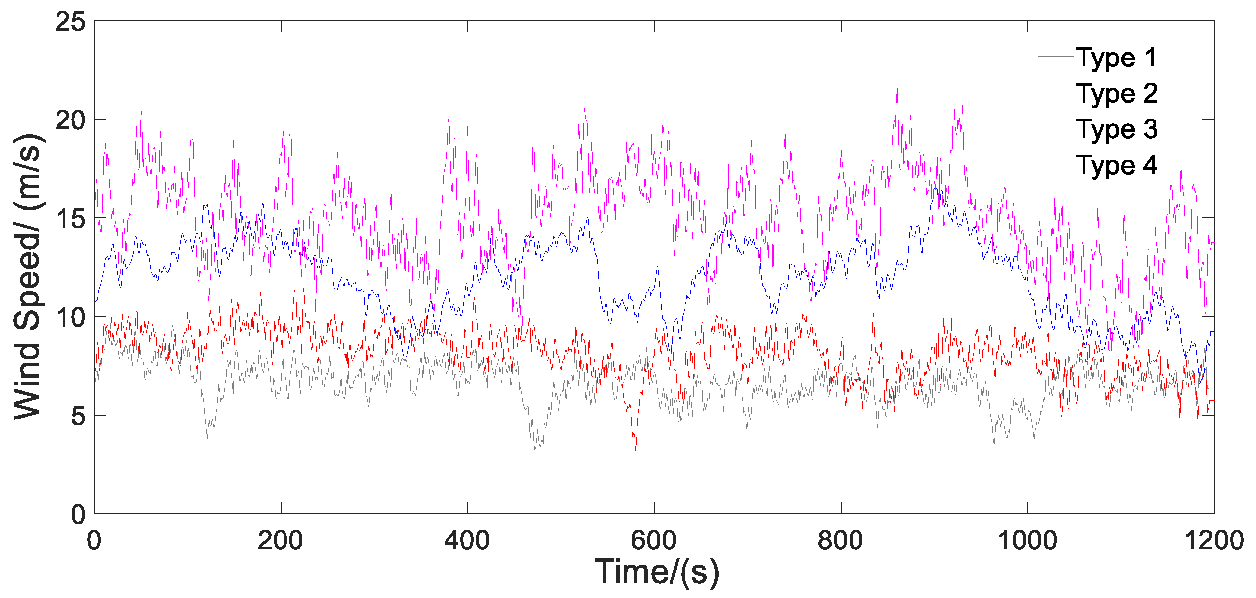
| Scenario Types | Mean Wind Speed (m/s)/Turbulence Intensity | ||
|---|---|---|---|
| 0–10 min | 10–20 min | 0–20 min | |
| Type 1 | 7.02/0.15 | 6.30/0.13 | 6.66/0.15 |
| Type 2 | 8.62/0.13 | 7.72/0.14 | 8.17/0.15 |
| Type 3 | 12.31/0.13 | 11.68/0.18 | 12.00/0.16 |
| Type 4 | 15.23/0.15 | 14.76/0.17 | 15.00/0.16 |
| Scenarios | MI Values of Two-Mass Model | |||||||||
| Tr–Tg | Tr–ωr | Tr–ωg | Tr–Tshaf | Tg–ωr | Tg–ωg | Tg–Tshaf | ωr–ωg | ωr–Tshaf | ωg–Tshaf | |
| Type 1 | 0.4856 | 0.4555 | 0.4552 | 0.5442 | 3.0705 | 3.1005 | 2.5336 | 5.5664 | 2.2144 | 2.2122 |
| Type2 | 0.6511 | 0.5651 | 0.5643 | 0.7068 | 2.2504 | 2.2601 | 2.5607 | 5.2716 | 1.9310 | 1.9292 |
| Type 3 | 1.3548 | 0.2447 | 0.2417 | 1.4188 | 0.2759 | 0.2751 | 3.2777 | 3.2968 | 0.2760 | 0.2746 |
| Type 4 | 0.1381 | 0.0479 | 0.0467 | 0.2241 | 0.0590 | 0.0601 | 0.6571 | 2.2888 | 0.0656 | 0.0658 |
| Scenarios | Normalized MI Values of Two-Mass Model | |||||||||
| Tr–Tg | Tr–ωr | Tr–ωg | Tr–Tshaf | Tg–ωr | Tg–ωg | Tg–Tshaf | ωr–ωg | ωr–Tshaf | ωg–Tshaf | |
| Type 1 | 0.0872 | 0.0818 | 0.0818 | 0.0978 | 0.5516 | 0.5570 | 0.4552 | 1 | 0.3978 | 0.3974 |
| Type2 | 0.1235 | 0.1072 | 0.1070 | 0.1341 | 0.4269 | 0.4287 | 0.4858 | 1 | 0.3663 | 0.3660 |
| Type 3 | 0.4109 | 0.0742 | 0.0733 | 0.4304 | 0.0837 | 0.0834 | 0.9942 | 1 | 0.0837 | 0.0833 |
| Type 4 | 0.0603 | 0.0209 | 0.0204 | 0.0979 | 0.0258 | 0.0263 | 0.2871 | 1 | 0.0287 | 0.0287 |
| Scenarios | Type 1 | Type 2 | Type 3 | Type 4 | |
|---|---|---|---|---|---|
| MI values | Ft–z | 1.3200 | 1.3080 | 1.1340 | 1.0938 |
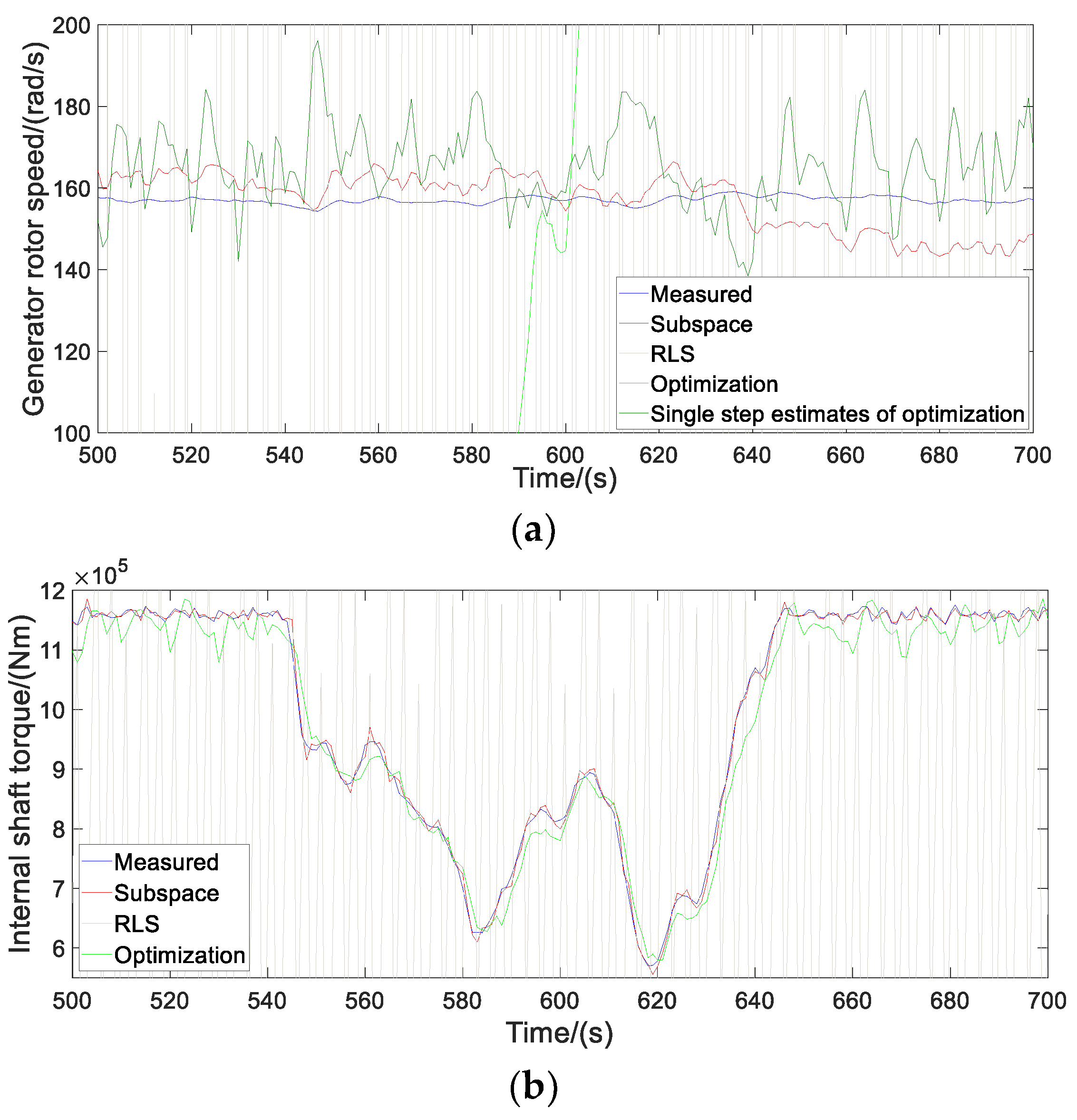
| Scenarios | Methods | nx, Jr, Jg, Astif, Bdamp | MSE | Fit-Percent | Stability |
|---|---|---|---|---|---|
| Type 1 | Subspace (MOESP) | nx = 10 | 7.964 × 10⁷ | −175.6%; 96.3% | −0.090 ± 0.951i; −0.284 ± 0.934i; −0.010 ± 0.627i; −0.866 ± 0.365i; 0.995; −0.437; Instability. |
| RLS | 3.544 × 10⁶; 1; 2.388 × 10⁵; 1.010 × 10⁷ | 4.214 × 10⁷ 3.073 × 10¹¹ | −2.785 × 10⁵% −130.064% | −1.458 × 10³; −2.363 × 10⁻²; 0; Instability. | |
| Optimization | 1.381 × 10⁵; 31.8; 2.101 × 10⁸; 1.655 × 10⁵ | 8.932 × 10⁸ | −1.37 × 10⁵%; 87.67% | −0.974±49.719i; −0. Stability. | |
| Type 2 | Subspace (MOESP) | nx = 10 | 8.883 × 10⁷ | 53.76%; 89.39% | 0.784 ± 0.521i; 0.259 ± 0.841i; −0.286 ± 0.824i; −0.712 ± 0.592i; −0.570; 0.994; Instability. |
| RLS | 5.776 × 10⁶; 1; 1.028 × 10⁵; −2.706 × 10⁶ | 7.466 × 10⁶; 5.547 × 10¹⁰ | −206.69%; −165.14% | 390.057; 0; 0.038; Instability. | |
| Optimization | 2.063 × 10⁵; 19.43; 2.062 × 10⁸; 1.702 × 10⁵ | 7.774 × 10⁸ | −1.69 × 10⁴%; 72.67% | −1.043 ± 50.266i; −0; Stability. | |
| Type 3 | Subspace (MOESP) | nx = 10 | 3.502 × 10⁷ | 90.11%; 89.53% | −0.878 ± 0.384i; −0.244 ± 0.939i; 0.435 ± 0.796i; 0.112 ± 0.974i; 0.997; 0.680; Instability. |
| RLS | 6.366 × 10⁶; 1; 6.920 × 10⁴; −4.531 × 10⁶ | 3.187 × 10⁶; 2.443 × 10¹⁰ | −1.527 × 10⁴% −176.42% | 653.17; 0; 0.0152; Instability. | |
| Optimization | 2.197 × 10⁵; 20.06; 2.153 × 10⁸; 1.901 × 10⁵ | 4.559 × 10⁸ | −1.768 × 10⁴%; 63.28% | −1.115 ± 50.241i; −0; Stability. | |
| Type 4 | Subspace (MOESP) | nx = 10 | 3.733 × 10⁸ | −449%; 70.33% | −0.789 ± 0.405i; −0.400 ± 0.791i; 0.084 ± 0.722i; 0.922 ± 0.362i; −0.845; 0.979; Instability. |
| RLS | 4.686 × 10⁷; 1; 2.767 × 10⁵; 1.620 × 10⁷ | 4.650 × 10⁷; 3.395 × 10¹¹ | −4.955 × 10⁵%; −794.72% | −2.336 × 10³; 0; −0.017; Instability. | |
| Optimization | 2.578 × 10⁵; 15.89; 1.954 × 10⁸; 2.087 × 10⁵ | 2.742 × 10⁹ | −2.734 × 10⁵%; 33.22% | −1.351 ± 50.274i; −0; Stability. |
| Identification Methods | Identification Condition Herein | Identification Results | Reason Analysis to Identification Results |
|---|---|---|---|
| Subspace (MOESP) | Direct identification under closed-loop condition without excitation signal | Valid: best fit-percent; instability | Black-box high-order model; closed-loop condition without excitation; no-self-balancing channel |
| RLS | Invalid: worst fit-percent; instability | Grey-box low-order model without process noise term; closed-loop condition without excitation; no-self-balancing channel | |
| Optimization | Valid: moderate fit-percent; stability | Grey-box low-order model without process noise term; no-self-balancing channel |
| Scenarios | Methods | nx, Mt, Dt, Kt | MSE | Fit-Percent | Stability |
|---|---|---|---|---|---|
| Type 1 | Subspace (CVA) | nx = 7 | 2.64 × 10⁴ | 55.53% | 0.698 ± 0.633i; −0.573 ± 0.620i; −0.071 ± 0.596i; 0.191; Instability. |
| RLS | 4.54 × 10⁴; −1.68 × 10⁴; 1.09 × 10⁶. | 8.70 × 10⁻⁵ | 74.55% | 0.185 ± 4.896i; Instability. | |
| Optimization | 1.16 × 10⁴; 1 × 10³; 1.099 × 10⁶. | 1.38 × 10⁻⁴ | 67.93% | −0.129 ± 9.728i; Stability. | |
| Type 2 | Subspace (CVA) | nx = 3 | 2.72 × 10⁻⁴ | 55.66% | −0.318 ± 0.589i; 0.535; Instability. |
| RLS | 2.88 × 10⁴; −8.93 × 10³; 1.13 × 10⁶. | 1.04 × 10⁻⁴ | 72.61% | 0.155 ± 6.25i; Instability. | |
| Optimization | 1.155 × 10⁴; 1 × 10³; 1.151 × 10⁶ | 1.49 × 10⁻⁴ | 67.33% | −0.130 ± 9.98i; Stability. | |
| Type 3 | Subspace (CVA) | nx = 7 | 2.20 × 10⁻⁴ | 48.09% | −0.549 ± 0.575i; −0.907 ± 0.203i; 0.707 ± 0.482i; 0.921; Instability. |
| RLS | 4.14 × 10⁴; −7.06 × 10³; 1.18 × 10⁶ | 9.24 × 10⁻⁵ | 66.52% | 0.0852 ± 5.343i; Instability. | |
| Optimization | 1.239 × 10⁴; 1 × 10³; 1.257 × 10⁶ | 1.63 × 10⁻⁴ | 55.53% | −0.121 ± 10.072i; Stability. | |
| Type 4 | Subspace (CVA) | nx = 3 | 6.72 × 10⁻⁴ | 38.35% | 0.623; −0.150 ± 0.347i; Instability. |
| RLS | 1.00 × 10⁴; 2.12 × 10³; 1.07 × 10⁶ | 1.79 × 10⁻⁴ | 68.35% | −0.106 ± 10.358i; Stability. | |
| Optimization | 1.116 × 10⁴; 1 × 10³; 1.127 × 10⁶ | 3.07 × 10⁻⁴ | 58.48% | −0.134 ± 10.049i; Stability. |
| Identification Methods | Identification Condition Herein | Identification Results | Reason Analysis to Identification Results |
|---|---|---|---|
| Subspace (CVA) | Direct identification under open-loop condition without excitation signal | Valid: worst fit-percent; instability | Black-box high-order model; insufficient excitation of operation data |
| RLS | Valid: best fit-percent; instability | Grey-box low-order model without process noise term | |
| Optimization | Valid: moderate fit-percent; stability | Grey-box low-order model without process noise term |
© 2019 by the authors. Licensee MDPI, Basel, Switzerland. This article is an open access article distributed under the terms and conditions of the Creative Commons Attribution (CC BY) license (http://creativecommons.org/licenses/by/4.0/).
Share and Cite
Chu, J.; Yuan, L.; Hu, Y.; Pan, C.; Pan, L. Comparative Analysis of Identification Methods for Mechanical Dynamics of Large-Scale Wind Turbine. Energies 2019, 12, 3429. https://doi.org/10.3390/en12183429
Chu J, Yuan L, Hu Y, Pan C, Pan L. Comparative Analysis of Identification Methods for Mechanical Dynamics of Large-Scale Wind Turbine. Energies. 2019; 12(18):3429. https://doi.org/10.3390/en12183429
Chicago/Turabian StyleChu, Jingchun, Ling Yuan, Yang Hu, Chenyang Pan, and Lei Pan. 2019. "Comparative Analysis of Identification Methods for Mechanical Dynamics of Large-Scale Wind Turbine" Energies 12, no. 18: 3429. https://doi.org/10.3390/en12183429
APA StyleChu, J., Yuan, L., Hu, Y., Pan, C., & Pan, L. (2019). Comparative Analysis of Identification Methods for Mechanical Dynamics of Large-Scale Wind Turbine. Energies, 12(18), 3429. https://doi.org/10.3390/en12183429