Heat to H₂: Using Waste Heat for Hydrogen Production through Reverse Electrodialysis

Abstract

This work presents an integrated hydrogen production system using reverse electrodialysis (RED) and waste heat, termed Heat to H${}_2$. The driving potential in RED is a concentration difference over alternating anion and cation exchange membranes, where the electrode potential can be used directly for water splitting at the RED electrodes. Low-grade waste heat is used to restore the concentration difference in RED. In this study we investigate two approaches: one water removal process by evaporation and one salt removal process. Salt is precipitated in the thermally driven salt removal, thus introducing the need for a substantial change in solubility with temperature, which KNO${}_3$ fulfils. Experimental data of ion conductivity of K${}^{+}$ and NO${}_3^{-}$ in ion-exchange membranes is obtained. The ion conductivity of KNO${}_3$ in the membranes was compared to NaCl and found to be equal in cation exchange membranes, but significantly lower in anion exchange membranes. The membrane resistance constitutes 98% of the total ohmic resistance using concentrations relevant for the precipitation process, while for the evaporation process, the membrane resistance constitutes over 70% of the total ohmic resistance at 40 ${}^{\circ }$C. The modelled hydrogen production per cross-section area from RED using concentrations relevant for the precipitation process is 0.014 ± 0.009 m${}^3$ h${}^{-1}$ (1.1 ± 0.7 g h${}^{-1}$) at 40 ${}^{\circ }$C, while with concentrations relevant for evaporation, the hydrogen production per cross-section area was 0.034 ± 0.016 m${}^3$ h${}^{-1}$ (2.6 ± 1.3 g h${}^{-1}$). The modelled energy needed per cubic meter of hydrogen produced is 55 ± 22 kWh (700 ± 300 kWh kg${}^{-1}$) for the evaporation process and 8.22 ± 0.05 kWh (104.8 ± 0.6 kWh kg${}^{-1}$) for the precipitation process. Using RED together with the precipitation process has similar energy consumption per volume hydrogen produced compared to proton exchange membrane water electrolysis and alkaline water electrolysis, where the energy input to the Heat to H${}_2$-process comes from low-grade waste heat.

1. Introduction

Renewable energy sources, like wind, solar, and wave energy, are often intermittent and not available when and where they are needed. The mismatch between energy production and consumption can be solved by introducing energy storage. One promising energy storage technology is hydrogen production through water electrolysis. Due to low-grade waste heat being readily available (20 TWh in Norway alone [1,2,3]), and the high power density from reversed electrodialysis [4], this article suggests a concept of using waste heat to produce hydrogen through reverse electrodialysis (RED).

In reverse electrodialysis energy is converted from potential energy stored in two solutions with different concentrations to electrical energy. The ions migrate from the concentrated to the dilute solution, and due to the alternating AEM and CEM, the anions and cations migrate in opposite directions inside the RED stack resulting in a net ionic current [5,6]. The concentration difference between the outlet solutions is lower than the concentration difference of the inlet solutions.

The first research on RED was conducted in the 1950s, where all the first experiments were done with NaCl concentrations similar to sea and river water [5,6,7,8]. The use of naturally occurring salt solutions is affordable but introduces bio-fouling of the membranes, or the use of energy-intensive pre-treatments of the solutions. Recirculating the salt solutions enable for a greater variety of salts, and by not using naturally occurring solutions (like sea and river), the bio-fouling of membranes can be avoided.

Closed-loop RED systems, using heat to separate the outlet solutions to the initial concentrations, have already been suggested in the literature. Tamburini et al. [9] suggested multiple separation techniques both for water and salt extraction. For water extraction they suggested separation by evaporation with multi-effect distillation and membrane distillation, using an azeotropic mixture to lower the evaporation temperature and forward osmosis [9]. Among the salt extraction techniques, Tamburini et al. [9] suggested a thermolytic salt (ammonium bicarbonate—AmB), where the salt is evaporated. The technique of evaporating the salt is also presented by other authors [10,11,12], where Raka et al. [10] found the energy needed per kg hydrogen produced to be 105–480 kWh. Membrane distillation as a separation technique with RED is also mentioned by Long et al., using sodium chloride [13].

Hydrogen production from RED has also been presented earlier. Nam et al. [14], Luo et al. [15] and Hatzel et al. [16] examined hydrogen production using AmB. Nam et al. produced hydrogen from microbial reverse electrodialysis cells (MRECs) and AmB [14]. Luo et al. optimised the cell stack further for MRECs and AmB [15]. Hatzel et al. examined hydrogen production using different operational currents, and compared it to the hydrogen production using the energy from RED together with an external water electrolysis cell [16]. In the area of salt removal for solutions, the most used salt is AmB.

Scope of This Paper

This paper describes two concepts for regenerating the concentrations used in RED by a thermal separation unit. A general system schematic is shown in Figure 1. The first concept is to precipitate salt from the dilute solution from RED, and the second concept is to evaporate water from the outlet concentrated solution. For the first concept, a salt with a pronounced saturation concentration temperature dependency (SCTD) is needed. The most common salt to use in RED, NaCl, does not have a sufficient SCTD, and thus the relevant concentrations will not give a sufficient voltage over the membrane using the precipitation system. A better alternative is KNO${}_3$ with a more significant change in solubility with temperature than NaCl, allowing for a larger concentration difference and a higher voltage over the membrane.

Most research on RED and ion exchange membranes (IEM) is reported for low NaCl concentrations or for AmB when waste heat is used for separation. As discussed in the next section, one of the larger contributors to the ohmic losses in RED is the ohmic resistance in the membranes. As a proof of concept for using KNO${}_3$ as salt in RED, conductivity measurements of AEM and CEM soaked in KNO${}_3$ at 23 ${}^{\circ }$C and 40 ${}^{\circ }$C were performed for concentrations close to saturation point, and compared with NaCl at the same concentrations and temperatures.

The current work is an extension and realization of preliminary concepts presented by the authors earlier [17]. The new and refined measurements of membrane conductivity presented in the following, combined with a more extensive theoretical framework enables lower uncertainties than what was presented before. Furthermore, an energy evaluation of the two processes allows for a broader comparison with other technologies, which was lacking in [17].

2. Concepts

This work presents a concept of a RED stack that recirculates the salt solutions in a closed loop. This requires the spent solutions to be recovered to their initial concentrations. The concepts presented here, rely on the use of low-temperature waste heat by employing phase change separation techniques, making low-grade heat the only consumable in the closed loop RED system. Due to different achievable concentration differences with the two techniques, the driving potential will differ, and thereby the peak power current and hydrogen production.

2.1. Salt Extraction by Precipitation

Thermal energy is removed from the dilute solution by precipitating salt from the solution. The salt slurry is transported from the dilute and added to the concentrated outlet solution where it dissolves, as illustrated in Figure 2. The transportation is envisioned to take place in an Archimedes pump or screw pump-based transport unit where a slurry of the precipitate is continuously in motion to avoid accumulation and solid precipitation of salt.

The amount of precipitated salt is dependent on the concentration of outlet dilute solution and solubility limit at the temperature the separation process is operated at. The concentration of the dilute inlet solution is therefore limited by the solubility of salt at the temperature used in the precipitation process. To minimise energy consumption while cooling, natural cooling systems can be used, e.g., seawater, at a temperature around 10 ${}^{\circ }$C.

The main contributor to the energy input needed for the precipitation concept is the heating of the salt slurry from the cooling (10 ${}^{\circ }$C) to the operating temperature in the RED stack (40 ${}^{\circ }$C), and the energy needed for dissolving the precipitated salt. To save energy, heat from the spent dilute solution, can be exchanged with the refreshed dilute solution, as shown by the heat flux, Q, in Figure 2.

2.2. Water Extraction by Evaporation

A sketch of a principle separation system using evaporation is shown in Figure 3. The spent concentrate solution is decompressed until the water evaporates with limited need for external thermal energy (Q). External low-grade heat, $Q_{\mathrm{H}}$, is added to the vapor to keep the gas form condensing before the gas is compressed. The gas transfers thermal energy to the spent concentrate solution to maintain the temperature, represented by Q in Figure 3. The evaporation will continue until the initial concentration in the solution is recovered, where the evaporated water is added to the outlet dilute solution from the cell. Pumps are needed in to depressurize the container.

This separation technique needs more substantial quantities of thermal energy than the precipitation, where the main energy consumption in this separation process is the evaporation of the water. The heat exchange is also a disadvantage for the energy calculation.

2.3. Temperature and Concentration Limitaitons

The limitation on the temperature stems from the membrane since commercial membranes can typically withstand maximum 40 ${}^{\circ }$C [18,19], some up to 80 ${}^{\circ }$C. The membranes used in the experiments reported here can only operate up to 40 ${}^{\circ }$C; therefore, 40 ${}^{\circ }$C is set as the operating temperature for the RED cell.

The concentration of the concentrated inlet solution in RED is limited by the solubility of the salt at the RED operating temperature (40 ${}^{\circ }$C), but due to more documented data in the literature at room temperature, all measurements and modeling are also carried out at 23 ${}^{\circ }$C for reference. The concentration for the dilute solution in RED, when using precipitation as the separation technique, is set by the solubility of the salt at the temperature used in the separation (10 ${}^{\circ }$C). The solubility of KNO${}_3$ and NaCl is found from CRC Handbook [20] (unit: wt% per mass solution) and calculated to molality (formula in [20]). The data is plotted in Figure 4.

The solubility for KNO${}_3$ is 2.11, 3.16 and 6.22 mol kg${}^{-1}$ at 10 ${}^{\circ }$C, 25 ${}^{\circ }$C and 40 ${}^{\circ }$C respectively, and 6.11, 6.15 and 6.22 mol kg${}^{-1}$ at 10 ${}^{\circ }$C, 25 ${}^{\circ }$C and 40 ${}^{\circ }$C respectively for NaCl. The relevant dilute concentration for the evaporation process is not limited by solubility, but optimised for maximum hydrogen production with modeling.

For the precipitation process using the most common salt for RED, NaCl, the dilute concentration should be 6.1 mol kg${}^{-1}$ and the concentrated concentration should be 6.2 mol kg${}^{-1}$, while using KNO${}_3$, the dilute concentration should be 2.1 mol kg${}^{-1}$ and the concentrated solution should be 6.2 mol kg${}^{-1}$ [20]. This corresponds to a driving potential that is over 60 times higher for KNO${}_3$ than that for NaCl (activity coefficient and permselectivity assumed equal to unity). However; the cost of KNO${}_3$ is almost twice that of NaCl [21], so other more affordable salts can be considered for future work. KNO${}_3$ was chosen as a proof of concept due to its significant change in saturation concentration with temperature and low cost. Other salts (such as CaCl${}_2$, NaOH and NaNO${}_3$) may also be relevant alternatives, granted they possess a high saturation concentration temperature dependency, reasonable cost and an improved permselectivity.

The concentration difference between the dilute and concentrated inlet solution can be larger in the evaporation system compared to the precipitation system, since there is no restriction on the dilute solution, improving the driving potential.

3. Theory

An illustration of a RED stack is given in Figure 5. Ions migrate both ways through the membranes, but more ions are available for migration from the concentrated solution to the dilute solution than vice versa, inducing a net ionic current of anions towards the anode and net current of cations towards the cathode.

By stacking the membranes, as shown in Figure 5, the voltage can be increased enough to enable water splitting (in the aqueous rinse solution) [22,23]. The water splitting reactions (also given in the figure) are:

$$\mathrm{Anode}:4{\mathrm{OH}}^{-}\to 2{\mathrm{H}}_2\mathrm{O}+{\mathrm{O}}_2+4{\mathrm{e}}^{-}$$

(1)

$$\mathrm{Cathode}:4{\mathrm{H}}_2\mathrm{O}+4{\mathrm{e}}^{-}\to 2{\mathrm{H}}_2+4{\mathrm{OH}}^{-}$$

(2)

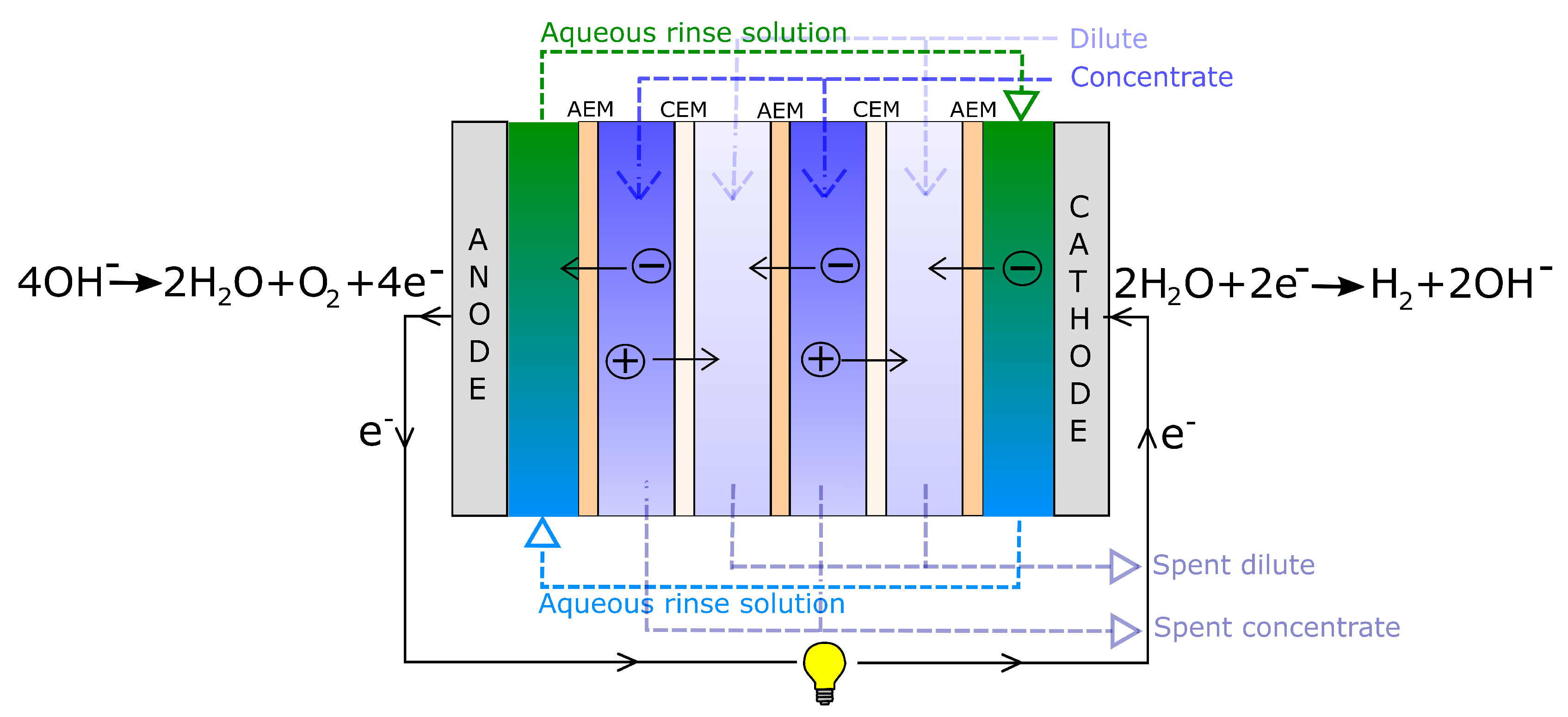
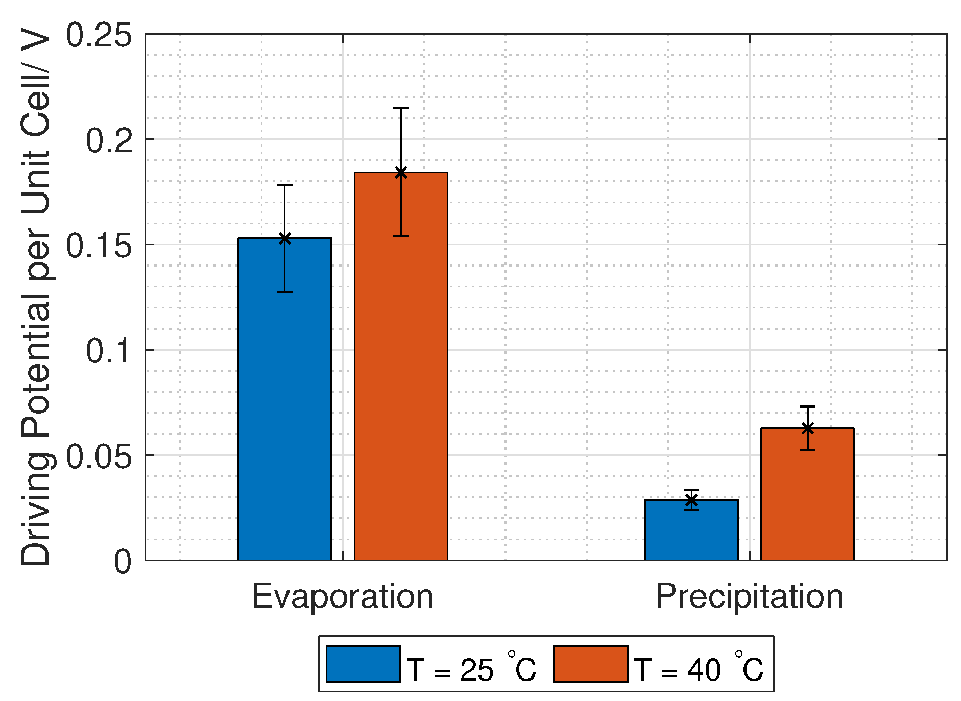
3.1. Driving Voltage

The open-circuit voltage (OCV) or the Donnan voltage, $E_{\mathrm{OCV}}$, over a RED unit cell is given by the Nernst equation:

$$E_{\mathrm{OCV}}=2\overline{\alpha }\frac{RT}{zF}\ln \left(\frac{b_{\mathrm{c}}{\gamma }_{\mathrm{c}}}{b_{\mathrm{d}}{\gamma }_{\mathrm{d}}}\right)$$

(3)

where $\overline{\alpha }$ is the mean permselectivity of the AEM and CEM in the unit cell, R is the ideal gas constant, T is the temperature in Kelvin, z is the valence number of the ions transported, F is Faraday’s constant, and $b_c$/$b_d$ and ${\gamma }_c$/${\gamma }_d$ are the concentration and activity coefficients of the concentrated/dilute solution, respectively [24].

The ratio of the activity coefficients are often assumed unity. However, due to concentrations close to the salt saturation point, the Stokes–Robinson equation is used for the calculation of the solution activity coefficient [25,26]:

$${\gamma }_{\pm }=exp\left(\frac{A{z}_{\pm }^2\sqrt{I}}{1+B{a}_{\mathrm{KNO}{}_3}\sqrt{I}}-\frac{h}{\nu }\ln (a_w)-\ln (|1+(M_{\mathrm{w}}(\nu -h)b|)\right)$$

(4)

where I is the ionic strength (reference: 1 mole salt per kg solvent). $z_{\pm }^2$ is the mean of the valence of the cation and anion (1 for KNO${}_3$), $M_{\mathrm{w}}$ is the molar mass of water (0.018 kg mol${}^{-1}$), $\nu$ is the number of ions per molecule (2 for KNO${}_3$) and $a_{\mathrm{KNO}{}_3}$ is the distance of the closest approach, which is dependent on the kinetic energy of the ions, thereby also the concentration and temperature of the solution. For simplicity, $a_{\mathrm{KNO}{}_3}$ is set constant with temperature and concentration, and found from curve fitting of data from Dash et al. and Marcos-Arroyo et al. [27,28] to Equation (4), and found to be 1.1 Å. The hydration number, h, is found to have a dependence on temperature and concentration [29]. Afanasiev et al. [30] suggest an exponential dependence on concentration and negligible dependence on temperature, while Onori [31] gives a linear dependence on concentration and states that the hydration number is dependent on temperature. For simplicity, h for KNO${}_3$ is set constant with temperature and concentration and taken to be the mean value from Lu et al. [32]: 5.

In Equation (4), A and B are temperature dependent constants given in Equation (5) (at 25 ${}^{\circ }$C $A=1.18$ (kg mol${}^{-1}$)${}^{1/2}$ and $B=3.29\times {10}^9$ (kg mol${}^{-1}$)${}^{1/2}$m${}^{-1}$ [33]).

$$\begin{array}{cc}\hfill A& ={(2\pi N_A{\rho }_w)}^{1/2}{\left(\frac{e_0^2}{4\pi {ϵ}_0{ϵ}_{r,w}{k}_{B}T}\right)}^{3/2}\hfill \\ \hfill B& =e{\left(\frac{2N_A{\rho }_w}{{ϵ}_0{ϵ}_{r,w}{k}_{B}T}\right)}^{1/2},\hfill \end{array}$$

(5)

where $N_A$ is Avogadro constant, ${\rho }_w$ is the density of the solvent (here water and set to constant 1000 kg m${}^{-3}$ for simplicity), $e_0$ is the elementary charge, ${ϵ}_0$ is permittivity of vacuum, $k_B$ is Boltzmann constant, and T is the temperature in Kelvin. ${ϵ}_{r,w}$ is the dielectric constant of the solvent [34] (here water) and given in Equation (6) (rewritten to use temperature in Kelvin instead of Celsius):

$${ϵ}_{r,w}=87.74-0.4008(T-273.2)+9.398\times 10{}^{-4}{(T-273.2)}^2-1.410\times 10{}^{-6}{(T-273.2)}^3$$

(6)

In Equation (4), $a_w$ is the water activity as a function of the salt concentration. Sangster et al. [35] measured the water activity in KNO${}_3$ solutions above 3 M and extrapolated the data for concentrations down to 0 M, giving a linear trend of the water activity. An approximation of the linear equation for the water activity in a KNO${}_3$ solution with molality b is given in Equation (7):

$$a_w=1-0.018b$$

(7)

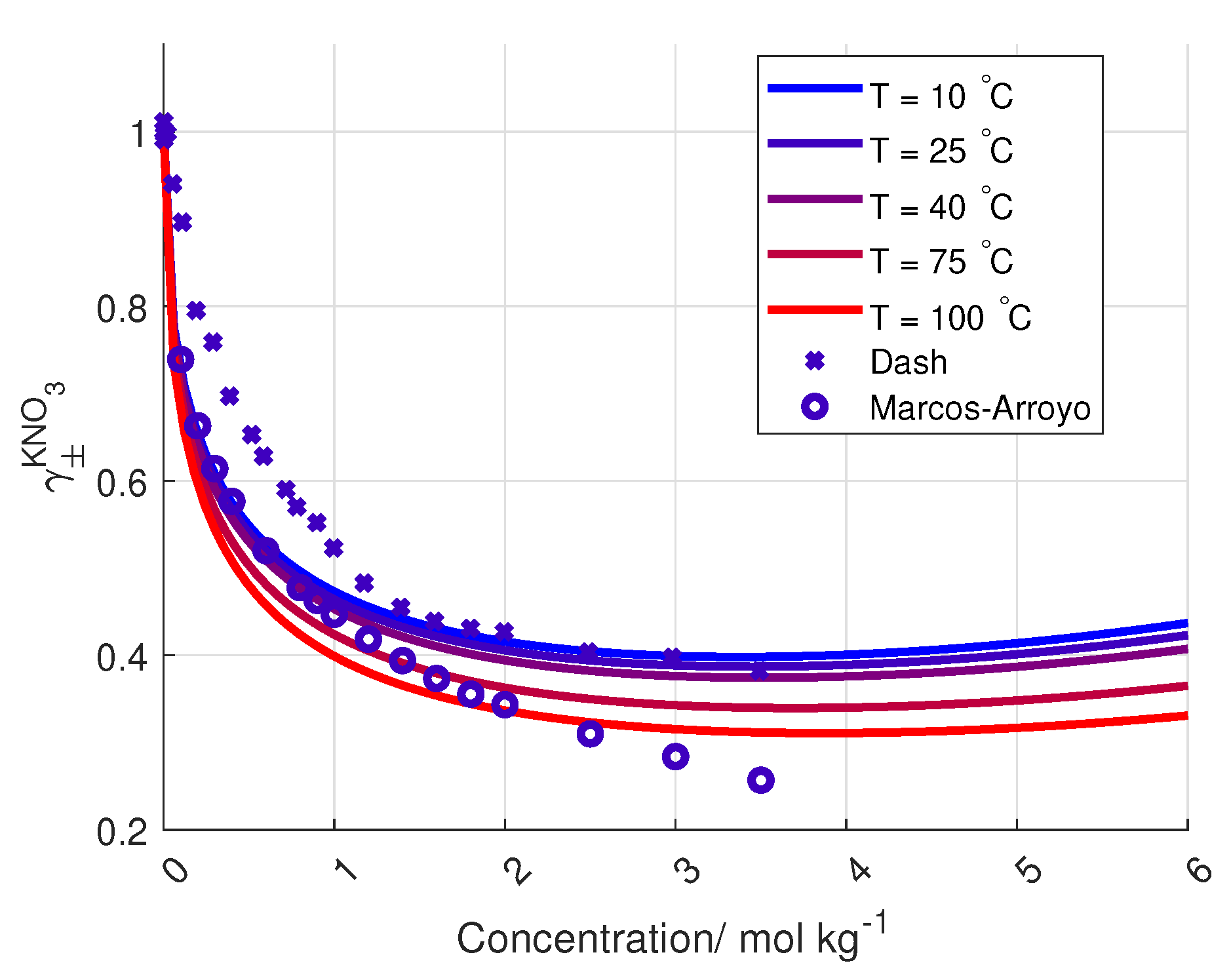
To the author’s knowledge, the activity coefficient of KNO${}_3$ is only measured at 25 ${}^{\circ }$C and up to salt concentrations of 3.5 mol kg${}^{-1}$, by Dash et al. and Marcos-Arroyo et al. [27,28]. Their experiments were similar, but Dash et al. used double junction reference electrode, while Marcos-Arroyo et al. used single junction. The modeled activity coefficient from Stokes–Robinson equation (Equation (4)) is plotted in Figure 6 together with the data from Dash and Marcos-Arroyo.

A reason for the deviation between the Stokes–Robinson equation and the measured activity coefficient of KNO${}_3$ from Dash et al. and Marcos-Arroyo et al. [27,28] is the assumption of no temperature or concentration dependency in the hydration number and the distance of closest approach in the model.

The apparent permselectivity, $\overline{\alpha }$ from Equation (3), increases with increasing concentration difference [36]. Krakhella et al. [37] measured FAS-50 and FKS-50 from Fumatech [18,19] at elevated NaCl concentrations, and found the permselectivity to vary (with concentrations) from 0.5 to 0.8. Ji and Geise [38] found that the permselectivity of two membranes dropped by approximately 2% when the temperature increased from 14 to 31 ${}^{\circ }$C. However, the Donnan voltage increases with increased temperature (Equation (3)), which was confirmed experimentally by Długołȩcki et al. and Van Egmond et al. [39,40], among others.

The total voltage in a RED stack is given in Equation (8):

$$E=E_{\mathrm{OCV}}{N}_{\mathrm{uc}}-E_{\mathrm{L}}-ri{N}_{\mathrm{uc}},$$

(8)

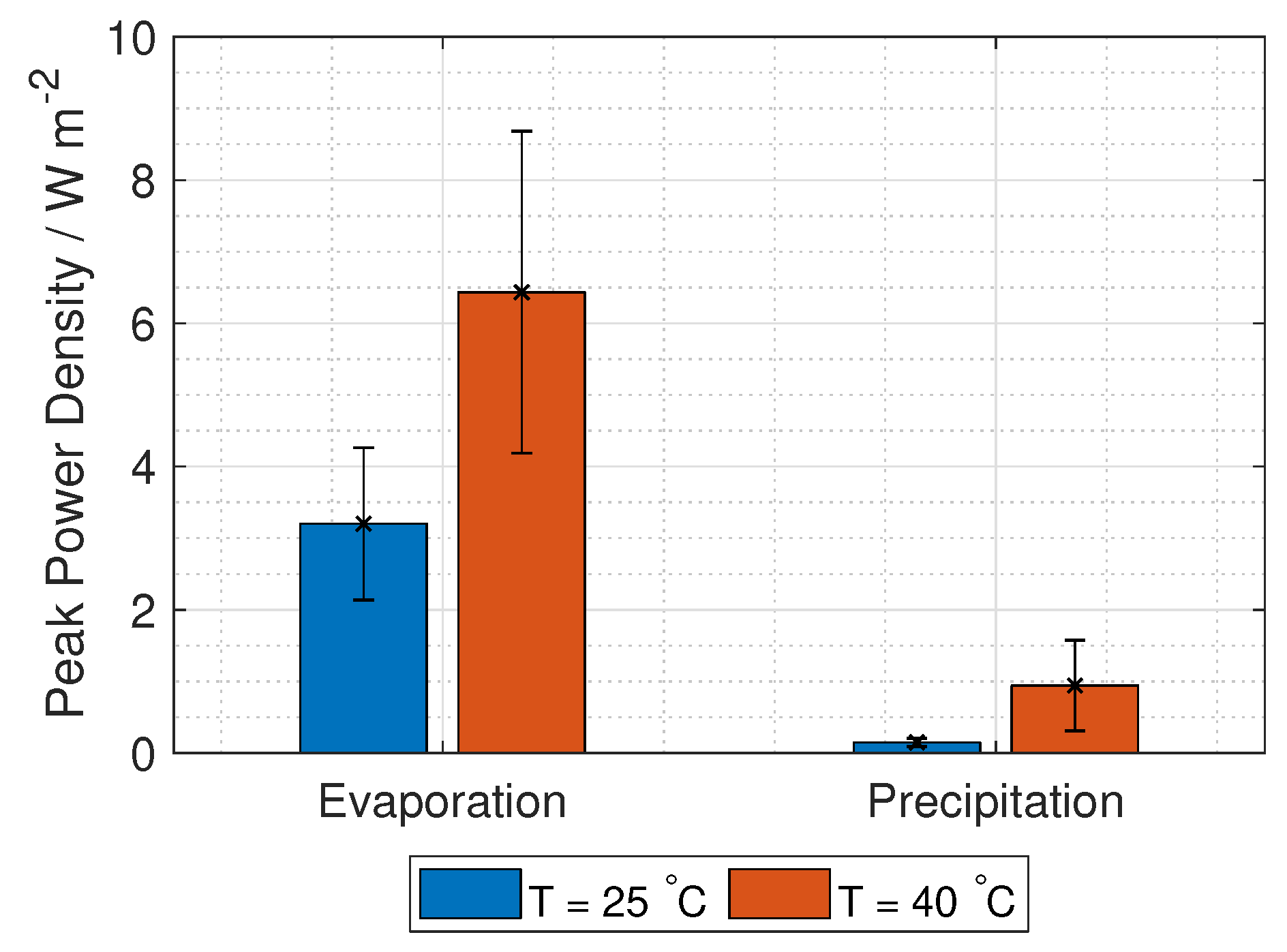
where $N_{\mathrm{uc}}$ is the number of unit cells, i is the current density per cross-section area and r is the unit cell area resistance given in Equation (14). $E_{\mathrm{L}}$ represents lumped electrode losses, including the activation overpotential losses and the ohmic losses at the electrodes. The power density gained from the RED stack is the stack voltage times the current, given in Equation (9):

$$P=E_{\mathrm{OCV}}{N}_{\mathrm{uc}}i-r{N}_{\mathrm{uc}}{i}^2$$

(9)

The voltage needed for hydrogen production is 1.23 V, while the current density is found at maximum power density, where the derivative of Equation (9) with respect to current density is zero. Using these two limitations, gives two equations with two unknowns (current and number of unit cells):

$$\begin{array}{cc}\hfill E_{\mathrm{OCV}}{N}_{\mathrm{uc}}-ri{N}_{\mathrm{uc}}& =(1.23+E_{\mathrm{L}})\mathrm{and}\hfill \\ \hfill E_{\mathrm{OCV}}{N}_{\mathrm{uc}}-2r{N}_{\mathrm{uc}}i& =0\hfill \end{array}$$

(10)

Solving Equation (10) gives the operating current density per unit cell area,

$$i_{P_{\max }}=\frac{E_{\mathrm{OCV}}}{2r_{\mathrm{uc}}},$$

(11)

and the number of unit cells needed:

$$N_{\mathrm{uc}}=\frac{2(E_{\mathrm{L}}+1.23)}{E_{\mathrm{OCV}}}.$$

(12)

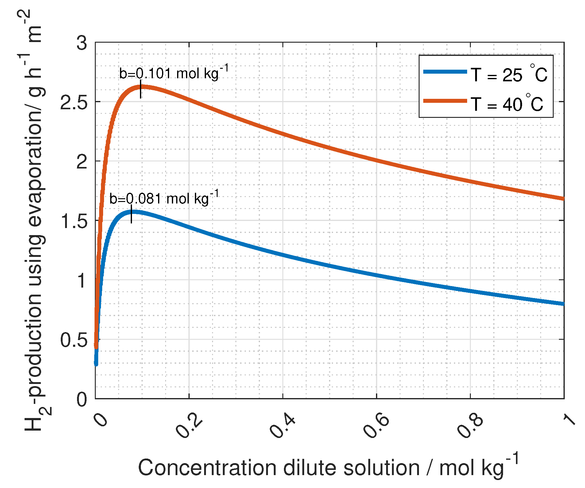
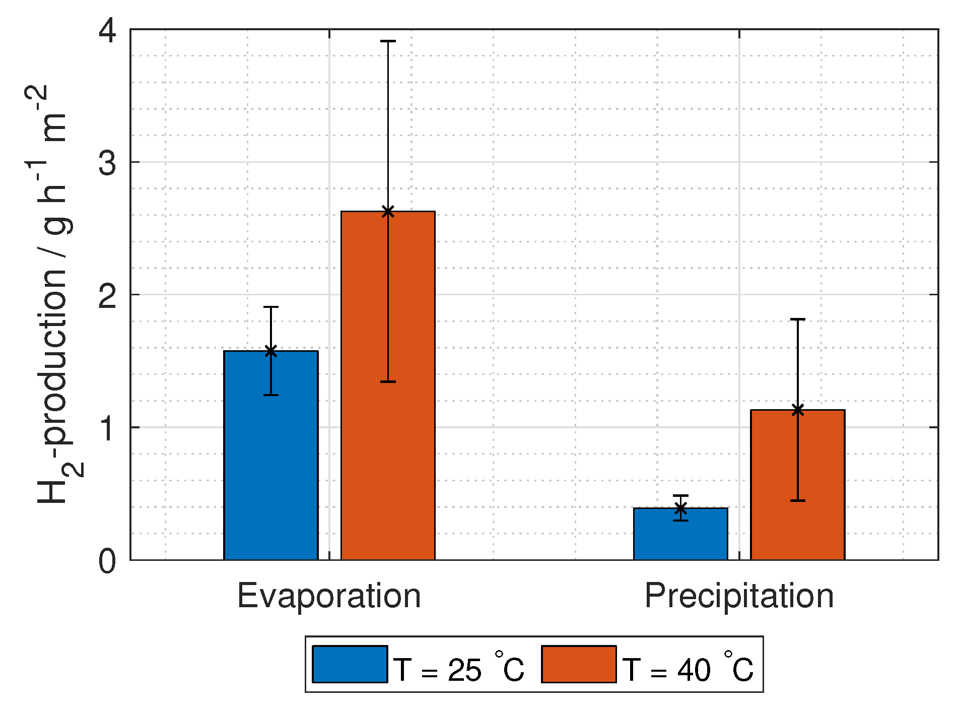
The hydrogen production in grams per hour per cross-section area is

$$m(H_2)=\frac{3600i_{P_{\max }}M}{2F}$$

(13)

where M is the molar mass of hydrogen gas (2.02 g mol${}^{-1}$).

It is important to highlight that the total ohmic losses of the RED stack, $ir{N}_{\mathrm{uc}}$, need to be (1.23 V + E${}_{\mathrm{L}}$) for all current densities and number of unit cells. This can be seen by solving Equation (10).

3.2. Losses

The losses considered in this work is the lumped electrode losses at the electrodes and the ohmic losses per unit cell. The Tafel losses are here considered to be a lumped loss of the activation potential and ohmic losses at the electrodes [24]. The operational current density for the RED stack is assumed small (<100 A m${}^{-2}$), where the activation and ohmic losses at the electrodes are approximately 0.10 V (see [24], p. 156).

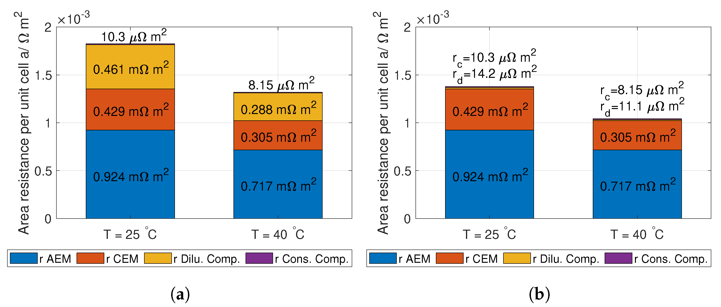
The ohimc losses are given in Equation (14):

$$r_{\mathrm{uc}}=\frac{d_{\mathrm{AEM}}}{{\rho }_{\mathrm{AEM}}(1-\beta )}+\frac{d_{\mathrm{CEM}}}{{\rho }_{\mathrm{CEM}}(1-\beta )}+\frac{d_{\mathrm{s}}}{{\rho }_{\mathrm{d}}{ϵ}^2}+\frac{d_{\mathrm{s}}}{{\rho }_{\mathrm{c}}{ϵ}^2},$$

(14)

where ${\rho }_{\mathrm{CEM}}$ and ${\rho }_{\mathrm{AEM}}$ are the conductivity of the AEM and CEM [S m${}^{-1}$] respectively, $d_{\mathrm{AEM}}$ and $d_{\mathrm{CEM}}$ is the thickness of the AEM and CEM, and $\beta$ is the spacer shadow (dimensionless) [39]. d is the thickness of the spacer, $ϵ$ (dimensionless) is the volume factor occupied by the spacer or the porosity (for no spacer: $ϵ$ = 1. For definition, see [41]). ${\rho }_{\mathrm{d}}$ and ${\rho }_{\mathrm{c}}$ are the conductivities of the dilute and concentrated solution respectively (S m${}^{-1}$). Theoretical values for ${\rho }_{\mathrm{d}}$ and ${\rho }_{\mathrm{c}}$ are deduced from conductivity measurement from [42], where the data is fitted to Kohlrausch’s equation (given in Hamann [43], p. 22) for 23 ${}^{\circ }$C and 40 ${}^{\circ }$C:

$$\begin{array}{cc}\hfill {\rho }_{23{}^{\circ }\mathrm{C},(\mathrm{Aq})}^{\mathrm{KNO}{}_3}& =k_{1,23{}^{\circ }\mathrm{C}}b-k_{2,23{}^{\circ }\mathrm{C}}{b}^{3/2}\hfill \\ \hfill {\rho }_{40{}^{\circ }\mathrm{C},(\mathrm{Aq})}^{\mathrm{KNO}{}_3}& =k_{1,40{}^{\circ }\mathrm{C}}b-k_{2,40{}^{\circ }\mathrm{C}}{b}^{3/2}\hfill \end{array}$$

(15)

where b is the molality, and the coefficients, $k_{1,i}$ and $k_{2,i}$, are given in

Table 1. Coefficients for Equation (15) with 95% conf. interval.

Name	Value
$k_{1,23{}^{\circ }\mathrm{C}}$	$12.2\pm 0.3$
$k_{2,23{}^{\circ }\mathrm{C}}$	$3.4\pm 0.2$
$k_{1,40{}^{\circ }\mathrm{C}}$	$15.8\pm 0.4$
$k_{2,40{}^{\circ }\mathrm{C}}$	$4.5\pm 0.2$

. $k_{1,i}$ is equivalent to the molar conductivity of infinite dilute solution, ${\mathsf{\Lambda }}_0$, and $k_{2,i}$ is a coefficient related to the stoichiometry of the electrolyte.

The ohmic losses in the flow compartment should be optimised with respect to hydrogen production (see Equation (13)). For wider compartments, the ohmic resistance increases, while pumping energy decreases. The ideal compartment width was found to be approximately 100 µm [44]. However, the compartment thickness in the simulations in this article is taken from Fumatechs ED-stack (given in Table 4). The solution concentration also contributes to the ohmic losses of the flow compartment, where a lower salt concentration increases the resistance (see Equation (15)). This would suggest higher concentrations on both sides of the membrane. However, a higher salt concentration gradient between the compartments enhances the RED driving potential (see Equation (3)). Optimising the solution resistance is needed for highest possible power density and hydrogen production, and varies with cell geometry and solution flow. When these factors are accounted for, the ionic resistance in the membranes is the main contributor to ohmic losses [8,45].

The energy losses in the RED-stack can be calculate from (unit Wh m${}^{-3}$ (hydrogen)):

$$W_{\mathrm{RED}-\mathrm{stack}}=E_{\mathrm{RED}-\mathrm{stack}}\frac{2pF}{3600RT},$$

(16)

where $E_{\mathrm{RED}-\mathrm{stack}}$ is the voltage loss over the RED-stack and p is the pressure (1 atm = 101,325 Pa).

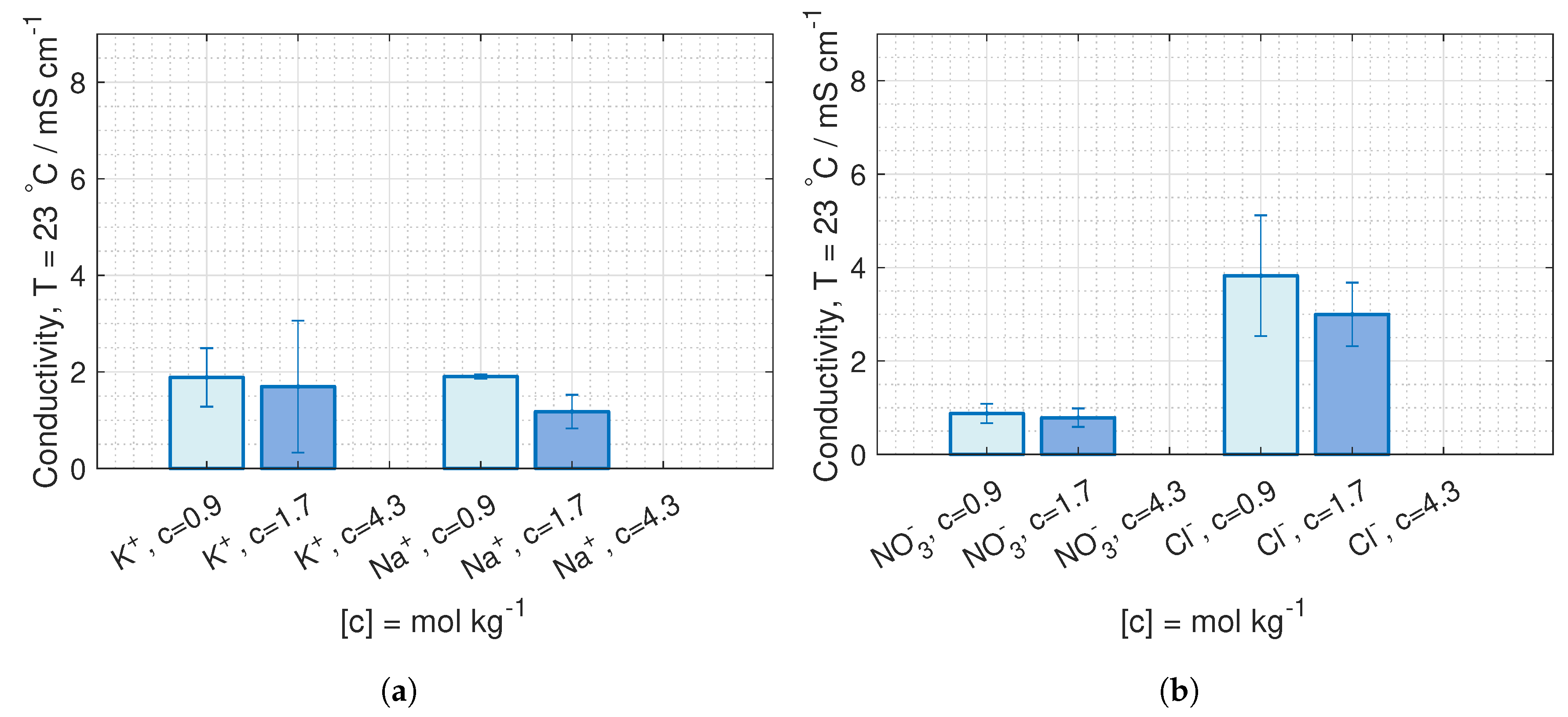
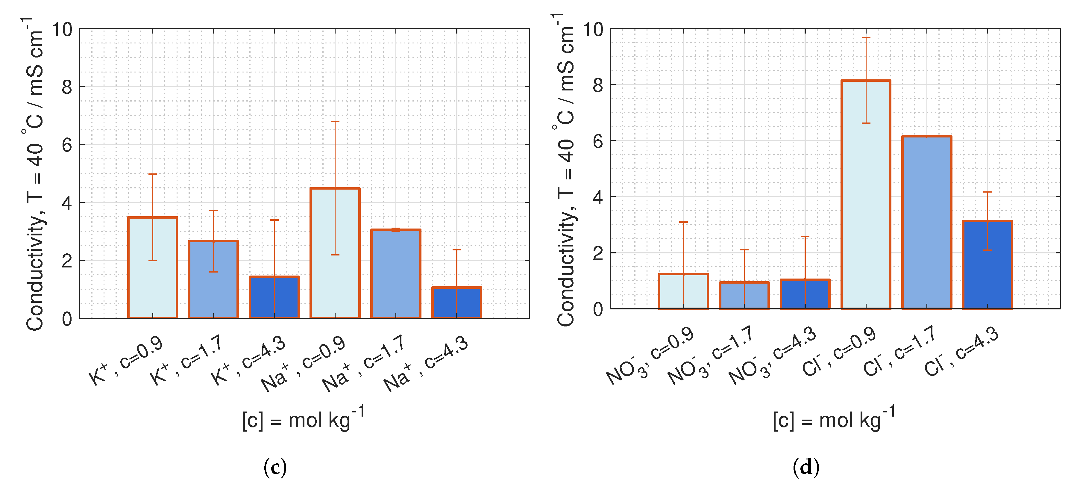
3.3. Ionic Membrane Conductivity

The ionic conductivity in the membrane in Equation (14), depends on the concentration and diffusion coefficient for both the counterions and co-ions [46] (Equation (8)). The concentration of counterions in the membranes is dependent on the fixed charges, and the amount of salt and water absorbed in the membrane pores [46,47]. The fixed charges are quantified by the ion exchange capacity (IEC) and are given as mmol g${}^{-1}$, and are constant (per membrane weight) with concentration. By increasing the IEC, the hydrophilicity of the polymer chains in the membrane increases and with it the water uptake. Water makes the membrane swell, reducing the density of the fixed charges in the membrane and increasing the adsorption of ions in the membrane. For the two membranes used in the experiments in this article, the IEC is 1.2–1.4 for CEM and 1.6–2.0 mmol g${}^{-1}$ for AEM [18,19], indicating a slightly better conductivity in AEM than CEM.

The swelling of the membrane is also affected by the difference between the membrane concentration and the external concentration. The water uptake in the membrane does not change much with the external concentration, but if the external concentration exceeds a certain limit (the Donnan concentration of the membrane), water can diffuse from the membrane to the solution, due to osmotic forces [46], decreasing the water and salt content inside the membrane. This concentration limit is around 0.07 M for Nafion 117 [48]. The result of the swelling and de-swelling, is a flux of water and dissolved salt into the membrane at low external concentration, and a flux of water from the membrane to the external solution at high external concentration, resulting in a strictly increasing concentration of both counterion concentration and co-ions in the membrane pores with external concentration [46].

The concentration of co-ions is also affected by the Donnan voltage over the membrane/solution interface, where a lower Donnan voltage between membrane and external solution leads to higher co-ion adsorption in the membrane [46].

The other factor affecting the ion conductivity in the membrane is the diffusion coefficient [46]. For NaCl the diffusion coefficient of the counterion is reported to decrease slightly with external concentration in CEM, while in AEM, the reported data showed no effect on the concentration [47]. However, the reported data from [47] is only conducted up to 1 M NaCl. For higher concentrations, the diffusion coefficient is believed to decrease with external concentrations, due to deswelling of the membrane. Kamcev et al. found the diffusion coefficient of the counterion always to exceed the co-ion, regardless of anionic or cationic membrane [46]. This indicates a faster transport at the fixed groups than in the pores.

Smaller particles should theoretically have a higher diffusion coefficient [49]. However, a smaller ionic radius has more charges per area on the surface of the ion, bringing more water molecules with it [49], increasing the hydraulic diameter. This results in two effects on the conductivity. The first effect is increased membrane wetting, where more water increases the conductivity. The second effect is that the physically larger ion will lower the diffusion coefficient. The crystalline and the hydrated radius of Na${}^{+}$, K${}^{+}$, Cl${}^{-}$ and NO${}_3^{-}$ are found from [49] and given in

Table 2. Crystal and hydrated radii of Na${}^{+}$, K${}^{+}$, Cl${}^{-}$ and NO${}_3^{-}$. Data obtained from [49].

	Na${}^{+}$	K${}^{+}$	Cl${}^{-}$	NO${}_3^{-}$
Crystal radius (nm)	0.101–0.117	0.138–0.149	0.181–0.194	0.179–0.189
Hydrated radius (nm)	0.178–0.358	0.201–0.331	0.195–0.332	0.340

.

3.4. Electrochemical Impedance Spectrocopy

In electrochemical impedance spectroscopy (EIS), an oscillating current (or potential) is applied to the system at a specific frequency, and the amplitude and phase shift of the voltage (or current) is measured. From this, the impedance of the system can be obtained.

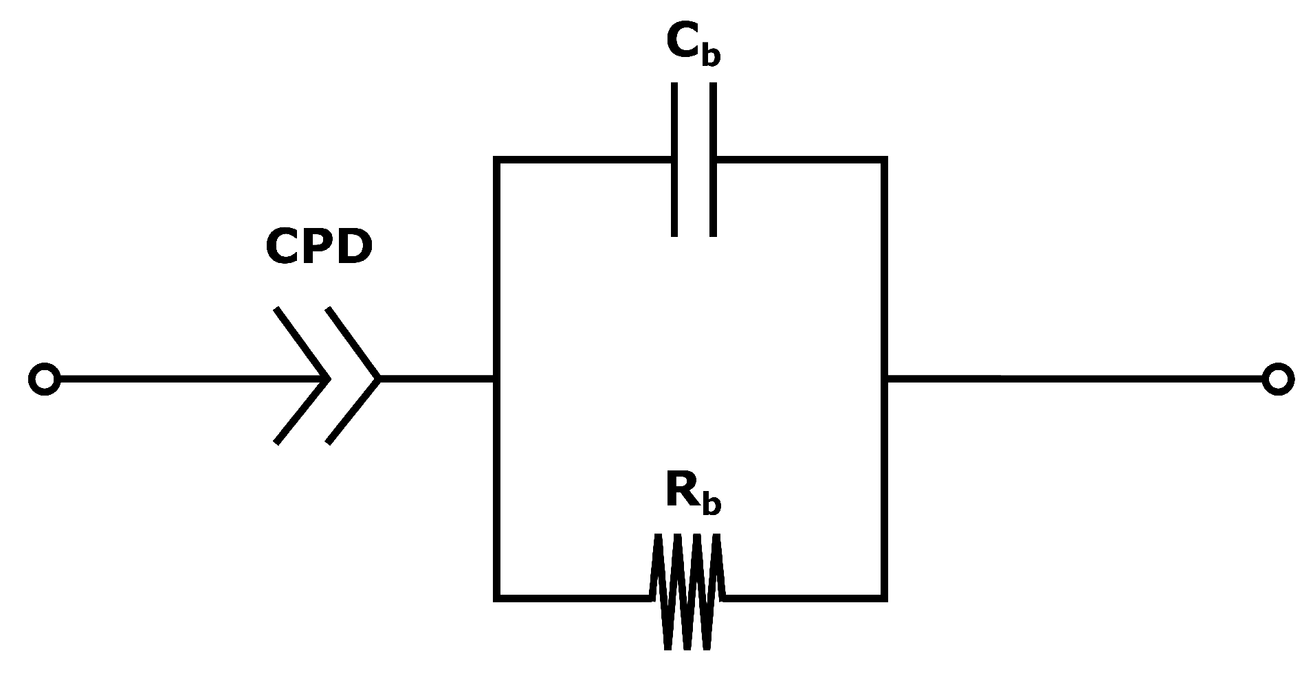
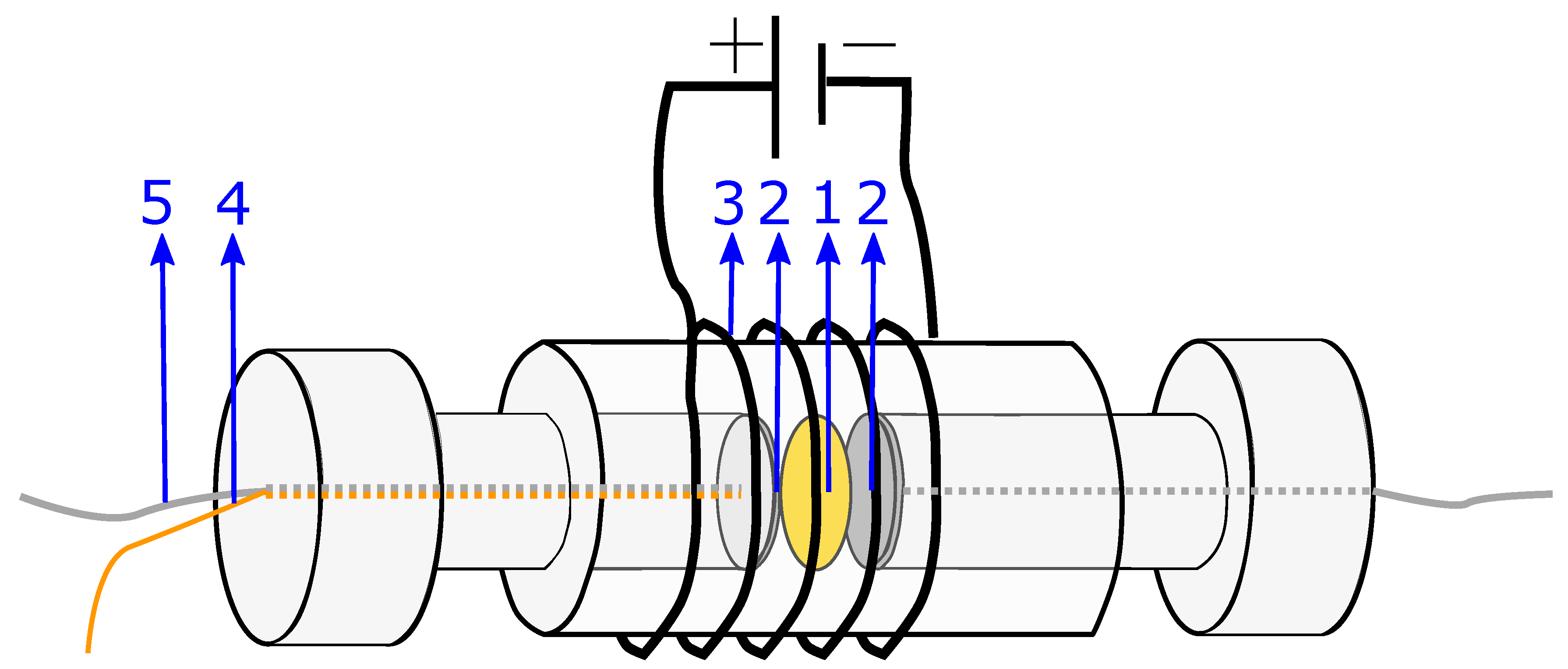
The system used for the present measurements is a membrane compressed between two electrodes (more details in Section 4.2). The equivalent circuit is therefore a series of the three components: the two electrode-membrane interfaces, and one membrane bulk impedance. The interface impedance between the membrane and the electrodes consists of a capacitive impedance ($C_{\mathrm{dl}}$), due to the double layer, in parallel with a resistance ($R_{\mathrm{dl}}$) representing the blocking interface. The membrane impedance is a bulk resistance ($R_{\mathrm{b}}$) in parallel with a capacitor ($C_{\mathrm{b}}$) due to the double layers building up in the pores in the membrane [50]. The total impedance is given in:

$$Z=\frac{1}{1/R_{\mathrm{dl},1}+i\omega C_{\mathrm{dl},1}}+\frac{1}{1/R_{\mathrm{b}}+i\omega C_{\mathrm{b}}}+\frac{1}{1/R_{\mathrm{dl},2}+i\omega C_{\mathrm{dl},2}},$$

(17)

Since no charge can pass the electrode/membrane interface, the interface impedance is merely capacitive [50]. Electrodes with a perfectly flat surface purely have a capacitive behaviour, although small irregularities in most electrodes lead to the use of a constant phase element (CPE) instead of a capacitor when analysing the impedance. The total impedance in Equation (17) can be simplified to:

$$Z=\frac{1}{{(i\omega C_{\mathrm{dl}})}^n}+\frac{1}{1/R_{\mathrm{b}}+i\omega C_{\mathrm{b}}}$$

(18)

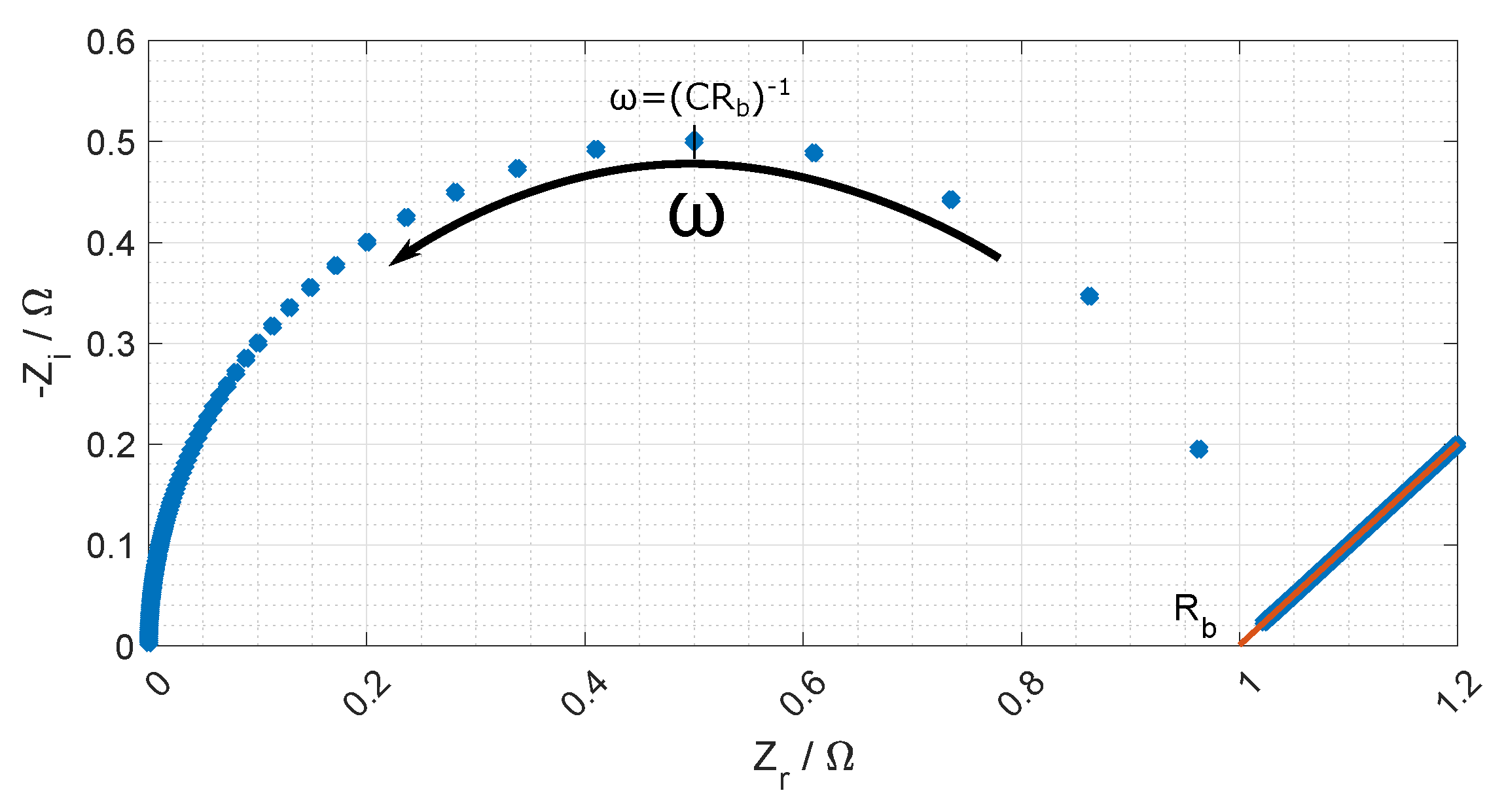
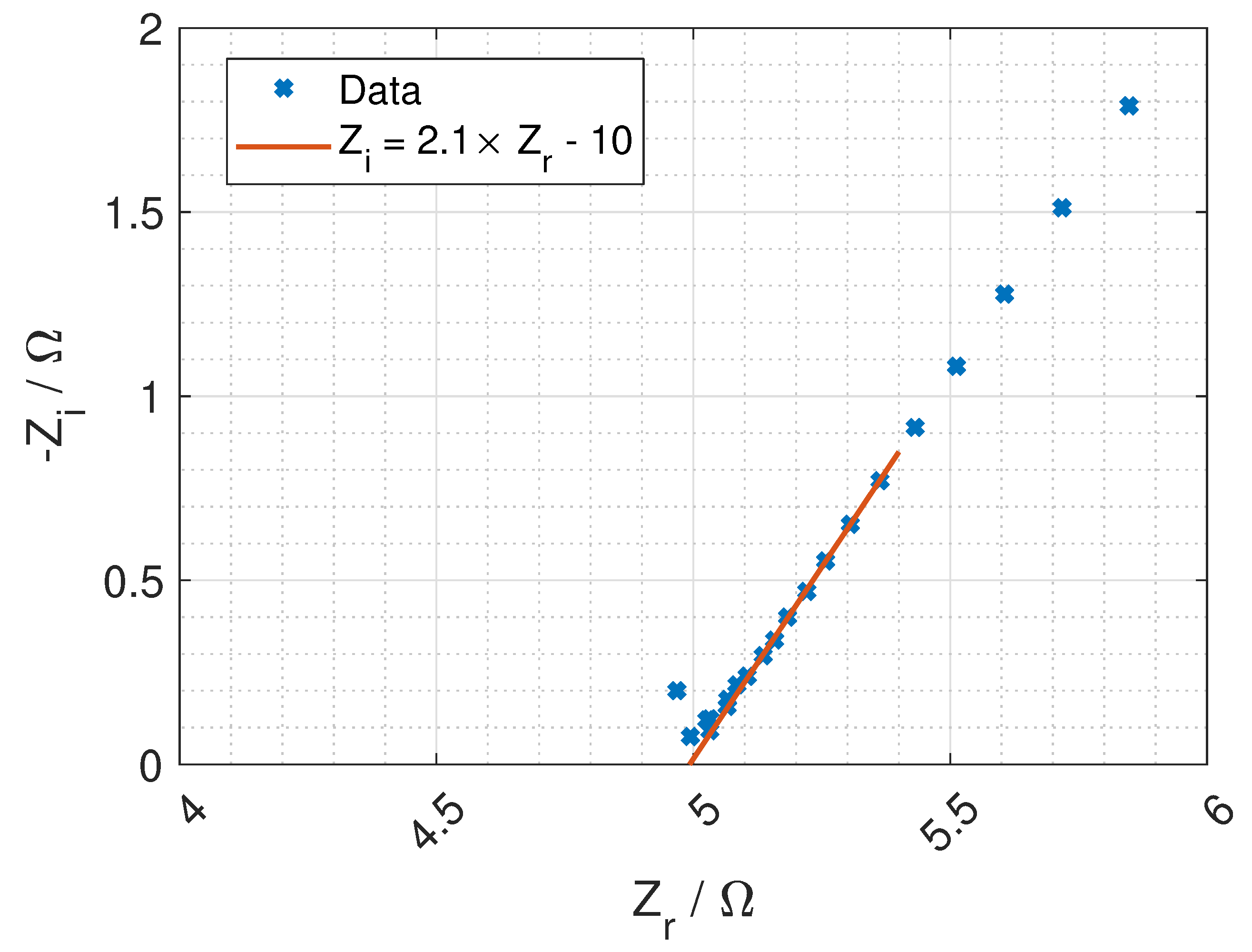
The equivalent circuit for the electrode membrane system is given in Figure 7 and a typical Nyquist plot of the resistance is given in Figure 8 where the bulk resistance in the membrane is marked.

When the frequency increases the contribution from the CPE decreases, and the contribution from the membrane increases. At a given frequency (≈1 MHz), the majority of the impedance is from the membrane resistance, and the ohmic membrane resistance can be found from the Nyquist plot (see Figure 8).

4. Experimental

Two membranes from Fumatech, FAS-50 and FKS-50 [18,19], with high permselectivity (in seawater at 25 ${}^{\circ }$C) are chosen for conductivity measurements with KNO${}_3$. The ion conductivity is measured at 23 ${}^{\circ }$C and 40 ${}^{\circ }$C, where the upper limit is due to possible degradation of the membranes above 40 ${}^{\circ }$C.

4.1. Membrane Preparation

FAS-50 and FKS-50 are delivered dry with the counter ions Br${}^{-}$ and H${}^{+}$, respectively, balancing the fixed charges [18,19]. After punching circular samples with a radius of 1 cm, six membranes were soaked in 500 mL of each concentration of KNO${}_3$ for minimum 36 h. To avoid precipitation of salt (e.g., a drop in temperature before measurements start), the membrane conductivity measurements are carried out at maximum of 4.3 mol kg${}^{-1}$. For comparison, both membrane types are soaked in the same concentration (mol kg${}^{-1}$) NaCl.

To measure the conductivity of only the counterions, the membranes could be rinsed in deionised water to remove salt solutions from the pores in the membranes. However, for our purpose, the ion conductivity of both the counterions and the ions dissolved in the pores in the membrane is of interest. The membranes are therefore not rinsed in deionised water before measurements.

After removed from the salt solution, the membrane thickness was measured in three different places for every sample with a micrometre and averaged, before they were placed in the setup described below.

4.2. Ion Conductivity Measurement

The cell used to measure membrane conductivity is illustrated in Figure 9. The setup contains two platinum disc electrodes with a radius of 1 cm and thickness of 1 mm, which the membrane sample is placed in between. Platinum wires are connected to the electrodes and mounted in a hard cylinder where the wires are emerging through the end. A tube is slid closely around the cylinders with the electrodes and membrane. Similar setups are standard in this kind of measurements [51,52].

To control the pressure on the membrane, the cylinder is placed in an (in-house made) screw clamp. The bolt (M6, hexagonal head) is tightened to a pressure of 2 Nm which is evenly distributed on the membrane due to the screw clamp.

For the measurements at 40 ${}^{\circ }$C, the setup is placed in a heating cabinet, where the temperature is maintained at 40 $\pm 1$ ${}^{\circ }$C throughout the experiment. For some of the experiments at 40 ${}^{\circ }$C, a heating wire was attached outside the cylinder to heat the system faster. This is illustrated in Figure 9.

Galvanostatic electrochemical impedance spectroscopy is performed with a two-electrode-setup using a Gamry Interface 5000E potentiostat. The settings used are given in

Table 3. Galvanostatic EIS settings for the potentiostat. * rms = root mean square, ≈0.7× peak current.

Variable	Value
DC current [A]	0
AC current [A rms] *	0.001
Initial frequency [Hz]	1 MHz
Final frequency [Hz]	5
Points/decade	10

.

To eliminate changes on the electrode surface in-between the experiments, both electrodes were polarised in 1 M H${}_2$SO${}_4$ from 0.1 to 1.6 V${}_{\mathrm{SHE}}$ until stable (no changes between the cycles), or minimum 30 cycles. The electrodes were also polished regularly. To account for inductance from the hardware, an experiment without the membrane sample was conducted, where the electrodes are compressed with the same pressure as used during the experiments with the membrane samples. The resulting impedance is subtracted from the impedance found with the membrane, using the software Echem Analyst.

As described in Section 3.4, the bulk resistance of the membrane, is found at the higher frequencies (after subtracting the blank cell), where the imaginary impedance is close to zero. In many cases, the Nyquist plot showed a straight line where it was easy to read of the bulk resistance. In the cases where the data was noisy at higher frequencies, a line was drawn through the lower linear data points to find the crossing point on the real axis, as shown in Figure 10.

For every concentration, temperature and membrane type (AEM and CEM), three experiments were run using 1, 3 and 5 membranes samples stacked inside the cell, to find the resistance for different thicknesses. The resistance was multiplied with the area of the membrane and plotted versus the thickness, where the slope of the graph is the resistivity ($\mathsf{\Omega }$m). The interface between the membranes is found to have a negligible impact on the resistance [17].

4.3. Power Density and Hydrogen Production

The unit cell power density is calculated from Equation (9), with all the input parameters given in

Table 4. Input values used to model power density and hydrogen production from RED.

Name	Symbol	Value
Solutions
Conc. dilute solution—evaporation	$b_{\mathrm{d}}^{\mathrm{eva}}$	calc. from H${}_2^{\max }$
Conc. dilute solution—precipitation (T = 10 ${}^{\circ }$C)	$b_{\mathrm{d}}^{\mathrm{pre}}$	2.11 mol kg${}^{-1}$ *
Conc. concentrated solution (T = [25 40] ${}^{\circ }$C)	$b_{\mathrm{c}}$	[3.79 6.22] mol kg${}^{-1}$ *
Temperature	T	[297 313] K
Flow volume per unit cell	$\mathsf{\Phi }$	$5.4\times 10$${}^{-5}$ kg s${}^{-1}$m${}^{-2}$ **
Membrane
Mean permselectivity CEM and AEM	$\overline{\alpha }$	0.63–0.96 ***
Conductivity AEM	${\rho }_{\mathrm{AEM}}$	measured
Conductivity CEM	${\rho }_{\mathrm{CEM}}$	measured
Thickness AEM	$d_{\mathrm{AEM}}$	$50\mathsf{\mu }$m
Thickness CEM	$d_{\mathrm{CEM}}$	$50\mathsf{\mu }$m
Cell geometry
Thickness spacer	$d_{\mathrm{s}}$	$155\mathsf{\mu }$m [37]
Spacer parameters
Shadow factor	$\beta$	0.35 [37]
Porosity	$ϵ$	0.84 [37]
Electrode
Lumped electrode losses	$E_{\mathrm{L}}$	0.10 V [24] (p. 156)
Constants
Molar mass KNO${}_3$	M	0.101 kg mol${}^{-1}$
Molar mass H${}_2$	M	0.00202 kg mol${}^{-1}$
Faraday’s constant	F	96,485 C mol${}^{-1}$
Universal gas constant	R	8.314 J K${}^{-1}$mol${}^{-1}$

* solubility limit for KNO${}_3$ at the given temperatures. ** recomended for the ED cell from Fumatech. *** no data for KNO${}_3$, but datasheet reported a mean of 0.96 for 0.5 M for NaCl [18,19] and Ref. [37] reported a mean permselectivity from 0.63–0.76 at elevated concentrations of NaCl.

. When plotting power density versus current density, a maximum power density can be found. The corresponding current density is used as an input to Equation (13).

As seen in Table 4 the concentrations of the concentrated solutions and the dilute solution used with the precipitation technique are set by the solubility limits. The ideal dilute concentration used with the evaporation process is set at maximum hydrogen production, which is found from calculations. The driving potential, solution resistance and power density are calculated for various dilute concentrations, giving one current density at maximum power for all the chosen dilute concentrations. The concentration giving the highest hydrogen production was chosen as the dilute concentration for the evaporation process.

4.4. Energy Used in Solution Separation

The mass balance in the two separations systems needs to be calculated to find the energy used. In the assumption that no water is crossing the membrane, the water content of both the inlet and outlet flow are the same, for both the concentrated and dilute solution (given in Table 4). The concentration (mol kg${}^{-1}$) of the outlet solutions from RED, is dependent on the hydrogen production:

$$\begin{array}{cc}\hfill b_{\mathrm{c}}^{\mathrm{outlet}}& =\frac{{\dot{n}}_{\mathrm{c}}^{\mathrm{inlet}}-2{\dot{n}}_{{\mathrm{H}}_2}}{{\mathsf{\Phi }}_{\mathrm{w}}}=\frac{b_{\mathrm{c}}^{\mathrm{inlet}}{\mathsf{\Phi }}_{\mathrm{w}}-2{\dot{n}}_{{\mathrm{H}}_2}}{{\mathsf{\Phi }}_{\mathrm{w}}}\hfill \\ \hfill b_{\mathrm{d}}^{\mathrm{outlet}}& =\frac{{\dot{n}}_{\mathrm{d}}^{\mathrm{inlet}}+2{\dot{n}}_{{\mathrm{H}}_2}}{{\mathsf{\Phi }}_{\mathrm{w}}}=\frac{b_{\mathrm{d}}^{\mathrm{inlet}}{\mathsf{\Phi }}_{\mathrm{w}}+2{\dot{n}}_{{\mathrm{H}}_2}}{{\mathsf{\Phi }}_{\mathrm{w}}}\hfill \end{array}$$

(19)

where ${\mathsf{\Phi }}_{\mathrm{w}}$ is the flow of water per second per cross-section area and $\dot{n}$ is the flow of moles per second per cross-section area.

In the precipitation system, a slurry of water and salt is removed from the spent dilute solution. The water removed can be compensated for by adding some of the spent concentrated solution back to the spent dilute solution. This is illustrated in Figure 11, where the water content in the slurry, ${\mathsf{\Phi }}_{\mathrm{w},2}$, is defined equal to the water content in the solution removed for the concentrated solution, ${\mathsf{\Phi }}_{\mathrm{w},1}$, and added back to the dilute concentration.

If the inlet concentration is to be kept constant, these two equation must apply, where ${\mathsf{\Phi }}_{\mathrm{w},2}$, is the water flux of the precipitated slurry and ${\mathsf{\Phi }}_{\mathrm{w},1}$ is the water flux added back to the spent dilute solution. The units are per time and cross-section area (flux):

$$\begin{array}{cc}\hfill \frac{{\dot{n}}_{\mathrm{c}}^{\mathrm{outlet}}-b_{\mathrm{c}}^{\mathrm{outlet}}{\mathsf{\Phi }}_{\mathrm{w},1}+b_{\mathrm{slurry}}{\mathsf{\Phi }}_{\mathrm{w},2}}{{\mathsf{\Phi }}_{\mathrm{w}}+{\mathsf{\Phi }}_{\mathrm{w},2}-{\mathsf{\Phi }}_{\mathrm{w},1}}& =b_{\mathrm{c}}^{\mathrm{inlet}}\hfill \\ \hfill \frac{{\dot{n}}_{\mathrm{d}}^{\mathrm{outlet}}+b_{\mathrm{c}}^{\mathrm{outlet}}{\mathsf{\Phi }}_{\mathrm{w},1}-b_{\mathrm{slurry}}{\mathsf{\Phi }}_{\mathrm{w},2}}{{\mathsf{\Phi }}_{\mathrm{w}}-{\mathsf{\Phi }}_{\mathrm{w},2}+{\mathsf{\Phi }}_{\mathrm{w},1}}& =b_{\mathrm{d}}^{\mathrm{inlet}}\hfill \end{array}$$

(20)

where $\dot{n}$ is the molar flux, b is the concentration and ${\mathsf{\Phi }}_{\mathrm{w}}$ is the mass flux of water (see Table 4 and Figure 11). The suffix $outlet$ and $inlet$ refers to the outlet and inlet solution from the RED stack, while c and d is the concentrated and dilute solution, respectively. The concentration of the slurry is set so that the mass of salt and water content is equal:

$$\frac{{\mathsf{\Phi }}_{\mathrm{salt}}}{{\mathsf{\Phi }}_{\mathrm{w}}}=1\to \frac{{\dot{n}}_{\mathrm{salt}}{M}_{\mathrm{salt}}}{{\mathsf{\Phi }}_{\mathrm{w}}}=1\to b_{\mathrm{slurry}}=\frac{1}{M_{\mathrm{salt}}}$$

(21)

Solving either of the equation in Equation (20) will give the mass flux of water in the salt slurry, ${\mathsf{\Phi }}_{\mathrm{w},2}$, and the water flux transferred from the concentrated to the diluted solution, ${\mathsf{\Phi }}_{\mathrm{w},1}$.

In the evaporation system, the water removed from the concentrated outlet solution needs to be added back for the dilute solution. This is illustrated in Figure 12. The water flux is taken to be the same as Fumatechs recommendations for their ED stack, and the outlet concentrations are calculated from Equation (19).

If the inlet concentration is to be kept constant, these two equations need to be solved, where ${\mathsf{\Phi }}_{\mathrm{w},1}$, is the water evaporated and added to the dilute solution, and ${\mathsf{\Phi }}_{\mathrm{w},2}$ is the water content of the solution added back to the spent concentrated solution. The units are per time and membrane area:

$$\begin{array}{cc}\hfill \frac{{\dot{n}}_{\mathrm{c}}^{\mathrm{outlet}}+b_{\mathrm{d}}^{\mathrm{outlet}}{\mathsf{\Phi }}_{\mathrm{w},2}}{{\mathsf{\Phi }}_{\mathrm{w}}-{\mathsf{\Phi }}_{\mathrm{w},1}+{\mathsf{\Phi }}_{\mathrm{w},2}}& =b_{\mathrm{c}}^{\mathrm{inlet}}\hfill \\ \hfill \frac{{\dot{n}}_{\mathrm{d}}^{\mathrm{outlet}}-b_{\mathrm{c}}^{\mathrm{outlet}}{\mathsf{\Phi }}_{\mathrm{w},2}}{{\mathsf{\Phi }}_{\mathrm{w}}+{\mathsf{\Phi }}_{\mathrm{w},1}-{\mathsf{\Phi }}_{\mathrm{w},2}}& =b_{\mathrm{d}}^{\mathrm{inlet}}\hfill \end{array}$$

(22)

The enthalpy for heating and evaporating water, and the enthalpy to dissolve KNO${}_3$ is given in

Table 5. Input enthalpy values used to model power density and hydrogen production from RED.

Name	Symbol	Value
Vaporizing water	$\Delta$H${}_{\mathrm{vap}.}$	$11.3$ Wh mol${}^{-1}$ (628 Wh kg${}^{-1}$) [53]
Heating water	$\Delta$H${}_{\mathrm{heating}}$	0.0209 Wh (mol K)${}^{-1}$ (1.16 Wh (K kg)${}^{-1}$)
Disolving KNO${}_3$ in water	$\Delta$H${}_{\mathrm{dissolve}}$	9.69 Wh mol${}^{-1}$ (538 Wh kg${}^{-1}$) [54]

.

5. Results and Discussion

The ion conductivity measurements revealed significant differences in ion conductivity for KNO${}_3$ and NaCl. The relevance of these results is demonstrated by implementing them into the described model of the hydrogen production from RED using concentrations relevant for precipitation and evaporation. This section contains results from the measured ion conductivity and the modelled data, and discussion of all the results.

5.1. Ion Conductivity Measurements

The ion conductivity of KNO${}_3$ and NaCl in CEM and AEM are plotted in Figure 13. The conductivity of KNO${}_3$ in CEM at both 23 ${}^{\circ }$C and 40 ${}^{\circ }$C are similar to the conductivity of NaCl. The ion conductivity in AEM is significantly lower for KNO${}_3$ than for NaCl at both 23 ${}^{\circ }$C and 40 ${}^{\circ }$C (Figure 13b,d).

Due to high deviations, a possible change in conductivity with concentrations can only be seen for NaCl, where the conductivity decreases with increased external concentrations. Even though the membrane concentration should increase with the external concentration (see Section 3.3), the water diffuses from the membrane to the external solution, both lowering the total amount of moving charges and decreases the diffusion coefficient.

The difference in conductivity between AEM and CEM could be due to a higher ICE in AEM than in CEM. This is the case for NaCl.

The general indication of an increase in conductivity with temperature can be due to increased swelling, resulting in a higher solution uptake.

5.2. Modeling of Hydrogen Production

As described in the experimental section, the dilute concentration used with the evaporation process is chosen from what gives the highest hydrogen production. The model of the hydrogen production for various concentrations is plotted in Figure 14 where the ideal dilute concentration for the evaporation process is found to be 0.081 and 0.101 mol kg${}^{-1}$ at 25 and 40 ${}^{\circ }$C respectively.

The permselectivity of the membranes in KNO${}_3$ is unknown but assumed to be between 0.96 and 0.63 (see Table 4). The driving potential from RED is found from Equation (3), with concentrations given in Table 4 and Figure 14, and activity coefficients given in Equation (4). The unit cell driving potential is plotted in Figure 15. The reason for the higher driving potential with concentrations relevant to evaporation compared to the potential using concentrations relevant for precipitation is only due to the increased concentration difference.

The membrane resistance of AEM and CEM at 23 ${}^{\circ }$C is taken to be the average over the measured concentrations (see Figure 13) due to no significant change in the conductivity. The relevant membrane ion conductivity for the modelling of the hydrogen is given in

Table 6. Measured membrane ion conductivity for the relevant mean concentration of KNO${}_3$ for the inlet to RED, 23 ${}^{\circ }$C and 40 ${}^{\circ }$C.

	${\mathit{\kappa }}_{\mathbf{AEM}}$	${\mathit{\kappa }}_{\mathbf{CEM}}$
23 ${}^{\mathbf{\circ }}$C	0.08 ± 0.01 S m${}^{-1}$	0.18 ± 0.07 S m${}^{-1}$
40 ${}^{\mathbf{\circ }}$C	0.11 ± 0.09 S m${}^{-1}$	0.20 ± 0.11 S m${}^{-1}$

.

The total theoretical ohmic resistance of the RED stack, including the measured membrane resistance, is given in Figure 16. The reason for the large difference in dilute solution resistance is the higher concentration in the inlet solutions used for the precipitation system compared to the evaporation system.

Given the open circuit potential in Figure 15, a lumped electrode loss of 0.1 V (see Table 4) and the unit cell ohmic resistance in Figure 16, the number of unit cells can be calculated from Equation (12). The results are given in

Table 7. The number of unit cells needed to have a total stack potential of 1.33 V and an operating current density at peak power.

	25 ${}^{\circ }$C	40 ${}^{\circ }$C
Precipitation	93$\pm 16$	43$\pm 8$
Evaporation	18$\pm 3$	15$\pm 3$

. The operation current density is calculated from Equation (11), and given in

Table 8. The operating current density of RED (see Equation (11)).

	25 ${}^{\circ }$C	40 ${}^{\circ }$C
Precipitation	10$\pm 2$ A m${}^{-2}$	30$\pm 18$ A m${}^{-2}$
Evaporation	42$\pm 9$ A m${}^{-2}$	70$\pm 34$ A m${}^{-2}$

.

The unit cell power density from RED is given in Figure 17. Due to uncertainties, both in the open circuit potential (permselectivity) and the membrane resistance, the propagation of uncertainty leads to correspondingly high uncertainties in the power density.

The predicted hydrogen production from the RED stack is given in Figure 18, where the production at 40 ${}^{\circ }$C using KNO${}_3$ is 2.6 ± 1.3 g h${}^{-1}$ m${}^{-2}$ (per cross-section area) for the evaporation process, and 1.1 ± 0.7 g h${}^{-1}$ m${}^{-2}$ (per cross-section area) for the precipitation process.

For comparison, proton exchange membrane water electrolysis (PEMWE) has a normal operation current density of 10 kA m${}^{-2}$ [55,56], resulting in a hydrogen production of 376 g h${}^{-1}$m${}^{-2}$. The cross-section area of RED needs to be minimum 160 times higher than the cross-section area in PEMWE to produce the same amount of hydrogen. However, the nature of the RED and PEMWE systems are different, as hydrogen is produced from electric power in PEMWE while the Heat to H${}_2$-system intends to use low-grade waste heat to produce hydrogen. The cell stack in the two systems also differs significantly: The bipolar plates, separating every unit cell in PEMWE, contribute to 80% of the weight and almost 50% of the cost in PEMWE [57]. In the RED-stack, there is no need for a unit cell separator. The membrane is also potentially cheaper in RED, where hydrocarbon material is used versus Nafion in PEMWE.

5.3. Energy Consumption and Cost

The energy losses in the RED stack, are the ohmic losses per unit cell and the lumped electrode losses. The calculation of these losses is carried out as described in Section 3.2. In the precipitation separation process, the majority of the energy is needed for heating the solution from 10 to 40 ${}^{\circ }$C and for dissolving the salt. In the evaporation separation process, the major energy consumption is in the evaporation of the water from the concentrated solution. In the calculation of the energy used per volume hydrogen produced, the hydrogen production at 40 ${}^{\circ }$C is used as a reference.

Using the hydrogen production from Figure 18 as input for Equation (19), the outlet concentrations from RED can be calculated, given in

Table 9. Inlet and outlet concentrations for the dilute and concentrated solutions.

Precipitation
Inlet conc. concentration	6.2 mol kg${}^{-1}$
Inlet dilute. concentration	2.1 mol kg${}^{-1}$
Outlet conc. concentration	6.1 mol kg${}^{-1}$
Outlet dilute concentration	2.2 mol kg${}^{-1}$
Evaporation
Inlet conc. concentration	6.2 mol kg${}^{-1}$
Inlet dilute. concentration	0.1 mol kg${}^{-1}$
Outlet conc. concentration	5.3 mol kg${}^{-1}$
Outlet dilute concentration	1.0 mol kg${}^{-1}$

. The difference in concentration from the inlet to the outlet solution from RED gives the amount of salt needed to add or remove from the outlet solutions to regenerate the original inlet concentrations.

Solving Equations (20) and (22), gives the mass fluxes as given in

Table 10. Mass fluxes in the two separation systems per cross-section area.

Specific Mass Flux	Mass Flux/kg h${}^{-1}$ m${}^{-2}$
Precipitation
Flux of water, ${\mathsf{\Phi }}_{\mathrm{w}}$	8.36
Flux intlet conc. solution (from RED)	13.6
Flux intlet dilute solution (from RED)	10.1
Flux outlet conc. solution (from RED)	13.5
Flux outlet dilute solution (from RED)	10.3
Flux of salt from dilute to conc. solution	0.295
Flux of water from dilute to conc. solution	0.295
Flux of solution from conc. to dilute solution	0.476
Evaporation
Flux of water, ${\mathsf{\Phi }}_{\mathrm{w}}$	2.92
Flux inlet conc. solution (from RED)	4.75
Flux inlet dilute solution (from RED)	2.95
Flux outlet conc. solution (from RED)	4.49
Flux outlet dilute solution (from RED)	3.21
Flux of water from conc. to dilute solution (eva.)	2.62
Flux of solution from dilute to conc. solution	2.88

. Using the enthalpies in Table 5 and the fluxes from Table 10, the energy used in the two Heat to H${}_2$-systems are given in

Table 11. Energy needed per volume hydrogen produced from RED using evaporation and precipitation at 40 ${}^{\circ }$C. * Due to the restriction on the ohmic and lumped electrode losses (see Section 3.1), there is no uncertainty.

Process	V	j	P	W	W
	V	A m${}_{\mathbf{cross}}^{-2}$	W m${}_{\mathbf{cross}}^{-2}$	kWh m${}^{-3}$	kWh kg${}^{-1}$
Evaporation
Reversible work	1.23	70$\pm 34$	86$\pm 42$	2.57	32.7
Electrode comp. loss	0.10 *	70$\pm 34$	7$\pm 3$	0.21	2.7
Ohmic loss RED-stack	1.33 *	70$\pm 34$	93$\pm 45$	2.78	35.3
Regen. heat (eva.)	24$\pm 10$	70$\pm 34$	1600 ± 1000	$49\pm 22$	600 ± 300
Total	26 ± 10	70 ± 34	1800 ± 1000	55 ± 22	700 ± 300
Precipitation
Reversible work	1.23	30$\pm 18$	86$\pm 42$	2.57	32.7
Electrode comp. loss	0.10 *	30$\pm 18$	3.0$\pm 1.8$	0.21	2.7
Ohmic loss RED-stack	1.33 *	30$\pm 18$	40$\pm 24$	2.78	35.4
Regen. heat needed	$0.341\pm 0.008$	30$\pm 18$	10$\pm 6$	$0.71\pm 0.02$	$9.1\pm 0.2$
Regen. heat (dissolve)	$0.94\pm 0.02$	30$\pm 18$	28$\pm 17$	1.96$\pm 0.04$	25.0$\pm 0.6$
Total	3.94 ± 0.02	30 ± 18	167 ± 52	8.23 ± 0.05	104.8 ± 0.6

.

For the evaporation process, 90% of the energy consumption is allocated to the evaporation of water. The total energy consumption is over ten times higher than the energy consumption per volume hydrogen produced with PEMWE (4.78 kWh m${}^{-3}$ [58], operating at 2 V) and alkaline water electrolyser (3 kWh m${}^{-3}$ [59]).

For the precipitation process, the majority of the losses are distributed evenly between the reversible work, the ohmic losses and the heating (dissolving of salt and heating of water). The total energy consumption of the RED and precipitation process is comparable to both PEMWE and alkaline water electrolysis.

The cost per kg of hydrogen produced can be estimated by including the membrane cost, which is assumed to be the most expensive part of the RED-stack materials [4], and the cost of the salt. This is a simplification, and for a future study other costs should be considered, e.g., the cost of the separation unit. Assuming a membrane price of 170 $ m${}^{-2}$ and a membrane lifetime of 4 years [10] the price for producing 1 kg of hydrogen is 55 $ and 370 $ for the evaporation and the precipitation process respectively. To compete with the cost of producing hydrogen using electrolysers, 4.2–14 $ kg${}^{-1}$ [60], the membrane price needs to cost less than 43 $ m${}^{-2}$ and 6.5 $ m${}^{-2}$ for the evaporation and precipitation process respectively. The cost of KNO${}_3$ is 78 $ kg${}^{-1}$, and the amount of salt inside the RED-stack is 1.3 kg m${}^{-2}$ and 4.7 kg m${}^{-2}$ for the number of unit cells relevant for the evaporation and precipitation system, respectively. Assuming the doubled amount of salt is needed for the entire Heat to H${}_2$-system and the system can operate for 100 years (membranes need to be changed more often), the cost of the salt is 0.043 $ and 0.371 $ per kg hydrogen produced using the evaporation and precipitation system respectively. In the present Heat to H${}_2$-system the price of the salt is negligible compared to the cost of the membranes. Raka et al. [10] found the contribution from heating to be over 50% of the total cost in a system similar to the one presented here. Obtaining the heat at an energy price of 0.15 $ per kWh [4], the cost of the heating per kg hydrogen produced is 100 $ using the evaporation process and 16 $ using the precipitation process.

6. Conclusions

Two separation techniques for outlet solutions from RED are presented. Due to the necessity of a large change in solubility with temperature, KNO${}_3$ is evaluated as a salt for the solutions used in RED. Ion conductivity is measured at 23 ${}^{\circ }$C and 40 ${}^{\circ }$C for one AEM and one CEM (FAS-50 and FKS-50) at three different concentrations. However, the conductivity of KNO${}_3$ did not change significantly with concentration. The conductivity for AEM was found to be 0.8 ± 0.1 mS cm${}^{-1}$ and 1.1 ± 0.9 mS cm${}^{-1}$ at 23 ${}^{\circ }$C and 40 ${}^{\circ }$C respectively, while for CEM the conductivity was found to be 1.8 ± 0.7 mS cm${}^{-1}$ and 2.5 ± 0.9 mS cm${}^{-1}$ at 23 ${}^{\circ }$C and 40 ${}^{\circ }$C respectively. Due to the low conductivity of NO${}_3^{-}$ in AEM other salts should be considered, e.g., CaCl${}_2$ and NaOH.

The driving force in RED using concentrations relevant to evaporation is 5 and 3 times higher than for the system relevant for precipitation at 25 ${}^{\circ }$C and 40 ${}^{\circ }$C respectively. However, due to lower dilute concentration in for the evaporation process, the resistance of the dilute compartment is 30 times higher for the concentration relevant for evaporation versus precipitation, increasing the total unit cell resistance by 30%.

Comparing the measured membrane resistance to the total unit cell resistance in RED, the membranes account for 98% of the total resistance using the precipitation process. For the evaporation process, the membrane resistance accounts for 70–80% of the total stack resistance. A decrease in the membrane resistivity with 50% would double the hydrogen production for the precipitation, while it would increase with 70% for the evaporation.

The predicted power density from RED in the two processes takes into account the assumed open circuit potential and the resistance. RED, using concentrations relevant for the evaporation process, can deliver seven times higher unit cell power density per cross-section area then RED using concentrations relevant for precipitation at 40 ${}^{\circ }$C.

The hydrogen production is calculated using the current at maximum power density, and a total RED stack potential of 1.33 V. The production of hydrogen using concentrations relevant for the evaporation process is 4 and 2 times higher than for concentrations relevant for the precipitation process at 25 ${}^{\circ }$C and 40 ${}^{\circ }$C respectively. From a cost perspective the evaporation process is preferable over the precipitation process due to a higher hydrogen production per membrane area, while from an energy demand perspective the precipitation process is the superior separation technique. The energy needed per cubic meter of hydrogen produced is 55 ± 22 kWh for the evaporation process and 8.22 ± 0.05 kWh for the precipitation process. The most common renewable source of hydrogen production today is PEMWE, which stands for 4% of the world’s total hydrogen production [61]. The results from the measurements and the modelling in this article present an alternative renewable way to produce hydrogen with an energy consumption comparable to PEMWE, where the input energy is otherwise lost low-grade waste heat.

References

1. From Waste Heat to a Resource. Available online: https://www.sintef.no/en/projects/from-waste-heat-to-a-resource/ (accessed on 1 July 2019).
2. Enova, S.F. Annual Report 2009—Results and Activities; Technical Report; Enova: Trondheim, Norway, 2009.
3. Brueckner, S.; Miró, L.; Cabeza, L.F.; Pehnt, M.; Laevemann, E. Methods to estimate the industrial waste heat potential of regions–A categorization and literature review. Renew. Sustain. Energy Rev. 2014, 38, 164–171. [Google Scholar] [CrossRef]
4. Jalili, Z.; Krakhella, K.W.; Einarsrud, K.E.; Burheim, O.S. Energy generation and storage by salinity gradient power: A model-based assessment. J. Energy Storage 2019, 24, 100755. [Google Scholar] [CrossRef]
5. Pattle, R. Production of electric power by mixing fresh and salt water in the hydroelectric pile. Nature 1954, 174, 660. [Google Scholar] [CrossRef]
6. Wick, G.L. Power from salinity gradients. Energy 1978, 3, 95–100. [Google Scholar] [CrossRef]
7. Weinstein, J.; Leitz, F. Electric power from differences in salinity: The dialytic battery. Science 1976, 191, 557–559. [Google Scholar] [CrossRef]
8. Lacey, R. Energy by reverse electrodialysis. Ocean Eng. 1980, 7, 1–47. [Google Scholar] [CrossRef]
9. Tamburini, A.; Tedesco, M.; Cipollina, A.; Micale, G.; Ciofalo, M.; Papapetrou, M.; Van Baak, W.; Piacentino, A. Reverse electrodialysis heat engine for sustainable power production. Appl. Energy 2017, 206, 1334–1353. [Google Scholar] [CrossRef]
10. Raka, Y.D.; Karoliussen, H.; Lien, K.M.; Burheim, O.S. Opportunities and challenges for thermally driven hydrogen production using reverse electrodialysis system. Int. J. Hydrog. Energy 2019. [Google Scholar] [CrossRef]
11. Luo, X.; Cao, X.; Mo, Y.; Xiao, K.; Zhang, X.; Liang, P.; Huang, X. Power generation by coupling reverse electrodialysis and ammonium bicarbonate: Implication for recovery of waste heat. Electrochem. Commun. 2012, 19, 25–28. [Google Scholar] [CrossRef]
12. Zhu, X.; He, W.; Logan, B.E. Influence of solution concentration and salt types on the performance of reverse electrodialysis cells. J. Membr. Sci. 2015, 494, 154–160. [Google Scholar] [CrossRef] [Green Version]
13. Long, R.; Li, B.; Liu, Z.; Liu, W. Hybrid membrane distillation-reverse electrodialysis electricity generation system to harvest low-grade thermal energy. J. Membr. Sci. 2017, 525, 107–115. [Google Scholar] [CrossRef]
14. Nam, J.Y.; Cusick, R.D.; Kim, Y.; Logan, B.E. Hydrogen generation in microbial reverse-electrodialysis electrolysis cells using a heat-regenerated salt solution. Environ. Sci. Technol. 2012, 46, 5240–5246. [Google Scholar] [CrossRef]
15. Luo, X.; Nam, J.Y.; Zhang, F.; Zhang, X.; Liang, P.; Huang, X.; Logan, B.E. Optimization of membrane stack configuration for efficient hydrogen production in microbial reverse-electrodialysis electrolysis cells coupled with thermolytic solutions. Bioresour. Technol. 2013, 140, 399–405. [Google Scholar] [CrossRef]
16. Hatzell, M.C.; Ivanov, I.; Cusick, R.D.; Zhu, X.; Logan, B.E. Comparison of hydrogen production and electrical power generation for energy capture in closed-loop ammonium bicarbonate reverse electrodialysis systems. Phys. Chem. Chem. Phys. 2014, 16, 1632–1638. [Google Scholar] [CrossRef]
17. Skilbred, E.S.; Krakhella, K.W.; Haga, I.J.M.; Pharoah, J.G.; Hillestad, M.; del Alamo Serrano, G.; Burheim, O.S. Heat to H2: Using Waste Heat to Set Up Concentration Differences for Reverse Electrodialysis Hydrogen Production. ECS Trans. 2018, 85, 147–161. [Google Scholar] [CrossRef]
18. FuelCellStore. Fumasep FAS-50; FuelCellStore: College Station, TX, USA, 2019. [Google Scholar]
19. FuelCellStore. Fumasep FKS-50; FuelCellStore: College Station, TX, USA, 2019. [Google Scholar]
20. Rumble, J.R. Aqueous solubility of inorganic compounds at various temperatures. In Handbook of Chemistry and Physics, 99th ed.; CRC: Boca Raton, FL, USA, 2018. [Google Scholar]
21. Inorganic Salts. Available online: https://www.sigmaaldrich.com/chemistry/chemistry-products.html?TablePage=16281684 (accessed on 22 August 2019).
22. Tufa, R.A.; Rugiero, E.; Chanda, D.; Hnàt, J.; van Baak, W.; Veerman, J.; Fontananova, E.; Di Profio, G.; Drioli, E.; Bouzek, K.; et al. Salinity gradient power-reverse electrodialysis and alkaline polymer electrolyte water electrolysis for hydrogen production. J. Membr. Sci. 2016, 514, 155–164. [Google Scholar] [CrossRef]
23. Kim, Y.; Logan, B.E. Hydrogen production from inexhaustible supplies of fresh and salt water using microbial reverse-electrodialysis electrolysis cells. Proc. Natl. Acad. Sci. USA 2011, 108, 16176–16181. [Google Scholar] [CrossRef] [Green Version]
24. Burheim, O.S. Engineering Energy Storage; Academic Press: Cambridge, MA, USA, 2017. [Google Scholar]
25. Stokes, R.H.; Robinson, R.A. Ionic hydration and activity in electrolyte solutions. J. Am. Chem. Soc. 1948, 70, 1870–1878. [Google Scholar] [CrossRef]
26. Glueckauf, E. The influence of ionic hydration on activity coefficients in concentrated electrolyte solutions. Trans. Faraday Soc. 1955, 51, 1235–1244. [Google Scholar] [CrossRef]
27. Dash, D.; Kumar, S.; Mallika, C.; Mudali, U.K. New data on activity coefficients of potassium, nitrate, and chloride ions in aqueous solutions of KNO3 and KCl by ion selective electrodes. ISRN Chem. Eng. 2012, 2012. [Google Scholar] [CrossRef]
28. Der Mar Marcos-Arroyo, M.; Khoshkbarchi, M.K.; Vera, J.H. Activity coefficients of sodium, potassium, and nitrate ions in aqueous solutions of NaNO3, KNO3, and NaNO3+KNO3 at 25 °C. J. Solut. Chem. 1996, 25, 983–1000. [Google Scholar] [CrossRef]
29. Pitzer, K.S.; Pabalan, R.T. Thermodynamics of NaCl in steam. Geochim. Cosmochim. Acta 1986, 50, 1445–1454. [Google Scholar] [CrossRef]
30. Afanasiev, V.N.; Ustinov, A.N.; Vashurina, I.Y. State of Hydration Shells of Sodium Chloride in Aqueous Solutions in a Wide Concentration Range at 273.15–373.15 K. J. Phys. Chem. B 2008, 113, 212–223. [Google Scholar] [CrossRef]
31. Onori, G. Ionic hydration in sodium chloride solutions. J. Chem. Phys. 1988, 89, 510–516. [Google Scholar] [CrossRef]
32. Lu, G.W.; Li, C.X.; Wang, W.C.; Wang, Z.H. Structure of KNO3 electrolyte solutions: A Monte Carlo study. Fluid Phase Equilibria 2004, 225, 1–11. [Google Scholar] [CrossRef]
33. Ribeiro, A.C.; Lobo, V.M.; Burrows, H.D.; Valente, A.J.; Sobral, A.J.; Amado, A.M.; Santos, C.I.; Esteso, M.A. Mean distance of closest approach of potassium, cesium and rubidium ions in aqueous solutions: Experimental and theoretical calculations. J. Mol. Liq. 2009, 146, 69–73. [Google Scholar] [CrossRef]
34. Malmberg, C.G.; Maryott, A.A. Dielectric constant of water from 0 °C to 100 °C. J. Res. Natl. Bur. Stand. 1956, 56, 1–8. [Google Scholar] [CrossRef]
35. Sangster, J.; Teng, T.; Lenzi, F. A general method of calculating the water activity of supersaturated aqueous solutions from ternary data. Can. J. Chem. 1973, 51, 2626–2631. [Google Scholar] [CrossRef]
36. Zlotorowicz, A.; Strand, R.V.; Burheim, O.S.; Wilhelmsen, Ø.; Kjelstrup, S. The permselectivity and water transference number of ion exchange membranes in reverse electrodialysis. J. Membr. Sci. 2017, 523, 402–408. [Google Scholar] [CrossRef] [Green Version]
37. Krakhella, K.W.; Seland, F.; Einarsrud, K.E.; Burheim, O.S. Electrodialytic Energy Storage System: IEM Permselectivity and Stack Measurements. Unpublished work.
38. Ji, Y.; Geise, G.M. The Role of Experimental Factors in Membrane Permselectivity Measurements. Ind. Eng. Chem. Res. 2017, 56, 7559–7566. [Google Scholar] [CrossRef]
39. Długołȩcki, P.; Gambier, A.; Nijmeijer, K.; Wessling, M. Practical potential of reverse electrodialysis as process for sustainable energy generation. Environ. Sci. Technol. 2009, 43, 6888–6894. [Google Scholar] [CrossRef]
40. Van Egmond, W.; Starke, U.; Saakes, M.; Buisman, C.; Hamelers, H. Energy efficiency of a concentration gradient flow battery at elevated temperatures. J. Power Sources 2017, 340, 71–79. [Google Scholar] [CrossRef] [Green Version]
41. Post, J.W.; Hamelers, H.V.M.; Buisman, C.J.N. Energy recovery from controlled mixing salt and fresh water with a reverse electrodialysis system. Environ. Sci. Technol. 2008, 42, 5785–5790. [Google Scholar] [CrossRef]
42. Isono, T. Density, viscosity, and electrolytic conductivity of concentrated aqueous electrolyte solutions at several temperatures. Alkaline-earth chlorides, lanthanum chloride, sodium chloride, sodium nitrate, sodium bromide, potassium nitrate, potassium bromide, and cadmium nitrate. J. Chem. Eng. Data 1984, 29, 45–52. [Google Scholar]
43. Hamann, C.; Hamnett, A.; Vielstich, W. Electrochemistry; Wiley-VCH: Weinheim, Germany, 2007. [Google Scholar]
44. Vermaas, D.A.; Guler, E.; Saakes, M.; Nijmeijer, K. Theoretical power density from salinity gradients using reverse electrodialysis. Energy Procedia 2012, 20, 170–184. [Google Scholar] [CrossRef] [Green Version]
45. Güler, E.; Elizen, R.; Vermaas, D.A.; Saakes, M.; Nijmeijer, K. Performance-determining membrane properties in reverse electrodialysis. J. Membr. Sci. 2013, 446, 266–276. [Google Scholar] [CrossRef]
46. Kamcev, J.; Paul, D.R.; Manning, G.S.; Freeman, B.D. Ion diffusion coefficients in ion exchange membranes: Significance of counterion condensation. Macromolecules 2018, 51, 5519–5529. [Google Scholar] [CrossRef]
47. Kamcev, J.; Doherty, C.M.; Lopez, K.P.; Hill, A.J.; Paul, D.R.; Freeman, B.D. Effect of fixed charge group concentration on salt permeability and diffusion coefficients in ion exchange membranes. J. Membr. Sci. 2018, 566, 307–316. [Google Scholar] [CrossRef]
48. Beers, K.M.; Hallinan, D.T., Jr.; Wang, X.; Pople, J.A.; Balsara, N.P. Counterion condensation in Nafion. Macromolecules 2011, 44, 8866–8870. [Google Scholar] [CrossRef]
49. Tansel, B.; Sager, J.; Rector, T.; Garland, J.; Strayer, R.F.; Levine, L.; Roberts, M.; Hummerick, M.; Bauer, J. Significance of hydrated radius and hydration shells on ionic permeability during nanofiltration in dead end and cross flow modes. Sep. Purif. Technol. 2006, 51, 40–47. [Google Scholar] [CrossRef]
50. Soboleva, T.; Xie, Z.; Shi, Z.; Tsang, E.; Navessin, T.; Holdcroft, S. Investigation of the through-plane impedance technique for evaluation of anisotropy of proton conducting polymer membranes. J. Electroanal. Chem. 2008, 622, 145–152. [Google Scholar] [CrossRef]
51. Barsoukov, E.; Macdonald, J.R. Impedance Spectroscopy: Theory, Experiment, and Applications; John Wiley & Sons: Hoboken, NJ, USA, 2005. [Google Scholar]
52. Müller, F.; Ferreira, C.A.; Azambuja, D.S.; Alemán, C.; Armelin, E. Measuring the proton conductivity of ion-exchange membranes using electrochemical impedance spectroscopy and through-plane cell. J. Phys. Chem. B 2014, 118, 1102–1112. [Google Scholar] [CrossRef]
53. Datt, P. Latent heat of vaporization/condensation. In Encyclopedia of Snow, Ice and Glaciers; Springer: Berlin/Heidelberg, Germany, 2011; p. 703. [Google Scholar]
54. Parker, V. Thermal Properties of Uni-Univalent Electrolytes; National Bureau of Standards: Washington, DC, USA, 1965; Volume 2, p. 66.
55. Carmo, M.; Fritz, D.L.; Mergel, J.; Stolten, D. A comprehensive review on PEM water electrolysis. Int. J. Hydrog. Energy 2013, 38, 4901–4934. [Google Scholar] [CrossRef]
56. Barbir, F. PEM electrolysis for production of hydrogen from renewable energy sources. Sol. Energy 2005, 78, 661–669. [Google Scholar] [CrossRef]
57. Tsuchiya, H.; Kobayashi, O. Mass production cost of PEM fuel cell by learning curve. Int. J. Hydrog. Energy 2004, 29, 985–990. [Google Scholar] [CrossRef]
58. Rashid, M.M.; Al Mesfer, M.K.; Naseem, H.; Danish, M. Hydrogen production by water electrolysis: A review of alkaline water electrolysis, PEM water electrolysis and high temperature water electrolysis. Int. J. Eng. Adv. Technol. 2015, 4, 2249–8958. [Google Scholar]
59. Zeng, K.; Zhang, D. Recent progress in alkaline water electrolysis for hydrogen production and applications. Prog. Energy Combust. Sci. 2010, 36, 307–326. [Google Scholar] [CrossRef]
60. Proost, J. State-of-the art CAPEX data for water electrolysers, and their impact on renewable hydrogen price settings. Int. J. Hydrog. Energy 2019, 44, 4406–4413. [Google Scholar] [CrossRef]
61. National Academy of Sciences. Carbon Capture and Storage—The rationale of carbon capture and storage from hydrogen production. In The Hydrogen Economy: Opportunities, Costs, Barriers, and R&D Needs; The National Academies Press: Washington, DC, USA, 2019. [Google Scholar]
Figure 1. Reversing the spent concentrations from RED using a thermal separation unit.
Energies 12 03428 g001
Figure 2. Illustration of the thermal separation unit (in Figure 1) using precipitation. Thermal energy is removed from the spent dilute solution (QC), to precipitate salt. Thermal energy (QH) is added to the spent concentrated solution after the salt slurry is added.
Energies 12 03428 g002
Figure 3. Illustration of the thermal separation unit (in Figure 1) using evaporation. The spent concentrated solution from RED, is decompressed to a lower evaporation temperature, before heat (Q) is added and water evaporated from the spent dilute solution. The vaporised water is heated (QH) and compressed, before thermal energy is exchanged with the spent concentrated, and the vaporised water is condensed back to a liquid and added to the spent dilute solutions.
Energies 12 03428 g003
Figure 4. Solubility dependency on temperature for NaCl and KNO 3 [20].
Energies 12 03428 g004
Figure 5. Illustration of a RED-cell. Hydrogen is produced at the cathode and oxygen at the anode.
Energies 12 03428 g005
Figure 6. Modeled activity coefficient for KNO 3 for different concentration and temperatures, together with measured activity coefficients from [27,28].
Energies 12 03428 g006
Figure 7. The equivalent circuit for a wet membrane between two electrodes.
Energies 12 03428 g007
Figure 8. Nyquist plot of Equation (18), and where the ohmic resistance of the membrane is found.
Energies 12 03428 g008
Figure 9. Sketch of the measurement cell for membrane conductivity, with (1) membrane sample(s), (2) platinum plates, (3) heating wire, (4) end of the thermocouple emerging from the cell, (5) end of the platinum wire (attached to the platinum plate) emerging from the cell.
Energies 12 03428 g009
Figure 10. Impedance data with linear fit to find the crossing of the real axis.
Energies 12 03428 g010
Figure 11. The mass flow in the precipitation system. Φ w , 1 is the water flow from the concentrated to the dilute solution, while Φ w , 2 is the water flow from dilute to concentrated solution. For no loss of water, Φ w , 1 Φ w , 2 .
Energies 12 03428 g011
Figure 12. The mass flow in the evaporation system. Φ w , 1 is the water flow from concentrated to the dilute solution, while Φ w , 2 is the water flow from the dilute to the concentrated solution. For no loss of water, Φ w , 1 Φ w , 2 .
Energies 12 03428 g012
Figure 13. Ion conductivity at 23 C in (a) CEM and (b) AEM, and at 40 C in (c) CEM and (d) AEM, with 95% confidence interval.
Energies 12 03428 g013aEnergies 12 03428 g013b
Figure 14. The change in the hydrogen production as a function of the dilute concentration in RED. The concentration of the concentrated inlet is set by the solubility limit at 25 and 40 C, 3.79 and 6.22 mol kg 1 .
Energies 12 03428 g014
Figure 15. Driving force for RED using concentrations relevant for the separation techniques evaporation and precipitation.
Energies 12 03428 g015
Figure 16. The total ohmic resistance in a RED unit cell at 23 °C and 40 °C using concentrations relevant for (a) evaporation and (b) precipitation. The calculation of the four contributions can be seen in Equation (14).
Energies 12 03428 g016
Figure 17. Power density from one RED unit cell (no tafel or electrode losses) per cross-section area using concentrations relevant for the separation techniques evaporation and precipitation.
Energies 12 03428 g017
Figure 18. Hydrogen production per hour and unit cell area from RED using concentrations relevant for the separation techniques evaporation and precipitation.
Energies 12 03428 g018