Article

District Heating Network Demand Prediction Using a Physics-Based Energy Model with a Bayesian Approach for Parameter Calibration

1
James Watt School of Engineering, the University of Glasgow, Glasgow G12 8QQ, UK
2
School of Engineering, the University of Edinburgh, Edinburgh EH9 3FB, UK
3
SP Distribution PLC, Glasgow G72 0HT, UK
*
Author to whom correspondence should be addressed.
Energies 2019, 12(18), 3408; https://doi.org/10.3390/en12183408
Submission received: 24 July 2019 / Revised: 31 August 2019 / Accepted: 2 September 2019 / Published: 4 September 2019
(This article belongs to the Section G: Energy and Buildings)

Abstract

:
Heat demand of a district heating network needs to be accurately predicted and managed to reduce consumption and emissions. Detailed thermal parameters are essential for predictions using physics-based energy models, but they are not always available or sufficiently accurate. To reduce the simulation time in calibration and the dependency of accurate data of buildings, this paper develops a prediction approach using a building energy model whose parameters are calibrated by Bayesian-based calibration method to match the recorded data of monthly heat demand. In the proposed calibration approach, an emulator is established to evaluate the untested values of thermal parameters using Bayesian method, and then use the evaluation results to search for the most suitable parameters value. The designed approach greatly accelerates the calibration speed. The method is used to calibrate a single parameter and multiple parameters of the building thermal energy models for a district heating network. After it has been verified with measured data, the developed calibration method is used to calibrate parameters of building energy models. The output of the calibrated model can predict the hourly building heat demand in district heating networks.

1. Introduction

The increasing consumption of fossil fuel has been causing global warming problems [1]. In cold regions, the demand of heat is much higher than that of electricity [2,3,4]. In the building sector, heat demand is much higher than in other sectors and constitutes 40% of the household energy consumption [5,6]. Accurate prediction of the heat demand of buildings is needed for the optimisation of heating networks, thermal comfort maintenance, and smart control of intelligent HVAC system [7]. The building energy models used to predict the heat dynamics of buildings can be categorised into engineering approaches, data-driven approaches, and their hybrids [8,9]. Engineering methods are developed with building energy simulators, which use bottom-up models to simulate the energy behaviour of a building. Based on the physical principles of heat transfer and engineering expertise, the bottom-up models can simulate the real thermal behaviour of a building according to the given ambient weather conditions, user behaviour and related building parameters including the heating area, thermal coefficients of walls, roof and windows, and solar heat gain coefficient. The thermal performance parameters depend on the thermal properties of various building material and the configurations of the building envelope [10]. Therefore, the building energy model is reliable to predict the heat demand only when the building thermal parameters of the model is well calibrated [11].
Many calibration methodologies have been proposed depending on different analytical methods and strategies [12,13,14,15]. Analytical calibration methods are widely used to adjust input parameters until simulation outputs match actual measurements [16]. In these studies, most calibration techniques are manual while only a few are automated. When the complexity of the building model increases, the reliability of the calibration method decreases [17]. In addition, these analytical calibration methods also require significant amounts of data from sensors, such as internal temperature or consumed energy in the target building [18]. On the other side, the input parameters have complicated internal interaction between each other since there are a large number of input parameters [17]. As a result, the analytical calibration method is unable to get available evidence to determine each parameter. Due to this issue, some sensitivity analysis approaches have been introduced to reduce the number of parameters to be adjusted in analytical calibration methods [19,20]. Alternatively, some studies have investigated simplified models with lumped parameters to reduce computational cost [21,22]. In many areas, such as in large parts of Scotland, a large number of historical buildings have been maintained and modified several times since they were built. It is a big challenge to measure the exact parameters of these historical buildings or to install sensors to obtain detailed data [23,24]. Besides, district heating networks (DHNs) usually contain tens to hundreds of different buildings, which increases the difficulty of collecting detailed data of each building for calibration.
Moreover, if the measured data is not accurate or the data is affected by uncertain factors, the traditional method could cause overfitting issue to the recorded data. The uncertainty analysis attracts particular research interests as the building energy models represent a simplification of reality. Mustafaraj et al. proposed a calibration method to ensure accuracy and to reduce the likelihood of errors for building energy efficiency simulation [25]. Heo et al. proposed a general theoretical approach to the uncertainty analysis in calibrating building energy simulation models [1]. Yang et al. devised a mesh generation strategy to calibrate the model parameters under high uncertainty by comparing the simulated indoor air temperatures to the experimental measurements [26]. Another possible approach is Bayesian calibration, which performs well in finding the posterior distribution of uncertain building parameters with noisy sensor data sets [9]. Yuan et al. used a Bayesian calibration approach to quantify the uncertainties associated with model parameter for representation improvement [27], and they also proposed a Gaussian Process (GP) based Bayesian method to simultaneously calibrate and rank input parameters of building energy simulation models to enable the efficient use of limited data sources [28]. However, the analysis of uncertainty aims to find the total distribution of the uncertainty statistically. The uncertainties still affect recorded data in time-series. Also, the traditional calibration method runs the simulation model many times until it matches the accurately recorded data of heat consumption. However, in calibrating the model of a DHN, the simulation time is extremely long as the network includes dozens of building models.
To solve these problems, this paper develops an approach to predict the heat demand of multi-buildings in a DHN accurately, even though the data source is limit and inaccurate. IES-VE software is used to build the bottom-up model of each building. The model parameters are then calibrated by Bayesian history matching (BHM) approach with monthly heat demand data. The BHM based calibration approach establishes an emulator to evaluate the untested points based on Bayesian method that calculates the conditional expectation and variance. The results from the emulator are then applied to exclude the implausible parameter ranges, as a result to find the point with the highest expectation from the non-implausible space for the next iteration. The expectation of the emulator describes the current belief of model behaviour to reduce the calibration time with reliable evidence. These steps are repeated until the stopping criteria are met. To demonstrate the proposed methodology, a case study has been conducted using the DHN at University of Glasgow main campus that includes thirty-four buildings connected to the heating network.

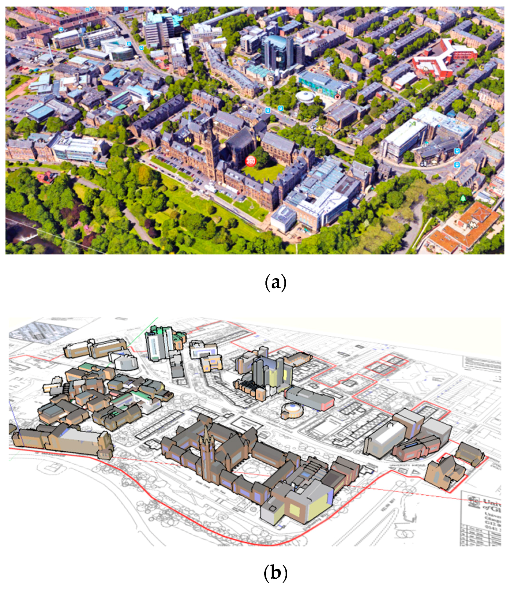
2. Modelling of Building Heat Demand in a District

The DHN at the main campus of the University of Glasgow is used as a case study, which has thirty-four buildings. It is modelled in a building energy simulator to predict its heat demand over the year. For this purpose, the campus map is used to determine the floor area and shape of each building. The buildings whose heat are supplied by the DHN are simulated in the model.
There are several commonly used simulators for this purpose. This paper chose Integrated Environmental Solutions Virtual Environment (IES-VE) to develop bottom-up models of buildings for thermal design and analysis as well as heating and cooling load simulation. IES-VE is an integrated system to simulate the building thermal behaviour using a proprietary engine called Apache. Compared with other building energy simulators, the strength of IES-VE is to correctly express the relationship between thermal zones and spaces defined in the building information bottom-up models [29].
The first step is to draw the building envelope either in the inbuilt toolbox or in an external building bottom-up modelling software. We established a building model of all buildings in SketchUp based on the campus map and then imported the bottom-up models into IES-VE for simulation of heating energy consumption. Apart from the floor area information given from the 2D campus map, the 3D information, such as the height of each building, shape of the roof, windows area, are measured from the 3D satellite image of Google global. The comparison between the satellite image and the completed building model of 34 buildings is shown in Figure 1. Then the completed model of buildings is imported into IES-VE, which can automatically detect the external walls, roofs, internal walls, and windows of each building from the bottom-up model.
There are many free parameters to be set in the IESVE simulation software. The most effective parameters are the building material and property parameters, which include the heat transfer coefficient (also called U-value) of external wall, windows, ground floor, roof, internal ceiling/carpeted floor and internal partitions. The building envelope of the bottom-up model separates the environment inside the building from the outside of the building and provides heat transfer resistance. The U-value is calculated in the software based on the basic building parameters, such as the thickness and materials. The external walls and roofs are the main surfaces for heat transfer between inside and outside environment, and there are many different types of materials in the structure [30,31]. The most common applied materials in construction are brick and blockwork, concretes, insulating materials, and plasters, as shown in Figure 2. In the exampled construction of the external wall, the better thermal resistance of the material causes faster temperature decreasing across layers.
In contrast to the walls that have a low heat transfer coefficient, the windows are transparent and have a higher heat transfer coefficient. Therefore, the size of windows is a significant parameter affecting the average U-values of the building envelope as well as the solar radiative coefficient in building heat demand estimation [32]. The window area can be easily measured for each building and is normally not a parameter that will be changed over time. For example, after hundreds of years, the thermal resistances of historical buildings could have significantly changed due to retrofitting, but their basic building information, such as floor area, building height and windows area, normally remains unchanged. The window area is a significant parameter affecting the building’s thermal behaviour, but it does not need to be calibrated like other parameters, such as the U-value of the ground floor, roof, internal ceiling/carpeted floor and internal partitions.
In addition to the building envelope parameters, the thermal gain also affects the building heat demand, including the thermal template of the HVAC system, the internal gain based on the number of people per unit area, the domestic hot water usage and the heating equipment operating hours. However, they are normally unpredictable and are also challenging to be accurately measured, especially in old buildings. In the IES-VE simulations, the parameters of these uncertain thermal gains were set as a constant ratio of the total heat demand of each building. The building management department provides the setting value from the documentation of plan. There are extra thermal gains inside the building as heat generated from people, computers, and other heating equipment. In addition, the building operating time also affects the total heat demand. For example, libraries are heated 24 h every day while office buildings usually are heated from 8 am to 6 pm. These parameters are variable depending on human activities and thus are difficult to predict accurately. The values set in IES-VE are chosen from the average usage of building template.
After defining the parameters, IES-VE will calculate the heat transfer coefficient of each part of the buildings from the above information and calculate the heat demand of every building with the imported weather profile and operating mode. The outdoor environment, especially the temperature, is the main factor that affects the building energy demand. In IES-VE model, the impact of weather is calculated together with the building heat transfer coefficient to get the heat demand as an output. The weather profile is obtained from the recorded database from the nearest weather station in Glasgow International Airport, including solar position, hourly temperature, humidity, and wind speed and direction. Since the campus is just around 7 miles away from the airport, the difference between the real weather condition around the heating network and the recorded weather profile from the airport is negligible. In the IES-VE simulation, the variation of the building envelope parameters, such as wall and glass thickness as well as their material and structure, will significantly affect the thermal behaviour of the building model and subsequently the heat demand. Therefore, the heat transfers related building parameters need to be carefully calibrated to force the model to match the thermal behaviour of the real buildings.
The ideal approach is to calibrate the thermal parameters of each building according to recorded data. However, this will require a large number of sensors to be installed in each building. It is not efficient for calibrating the models of multi-buildings due to extremely high costs. An alternative method is to use lumped parameters for all buildings, and only one sensor is required to record the heat demand of the whole heating network. While the usage of lumped parameters could reduce the accuracy of the heat demand of a single building, in a DHN with tens to hundreds of buildings, the accuracy of a single building will not have a significant impact on the overall heat demand of the network. What is more, the complexity and computational load in model calibration will be significantly reduced in calibrating the lumped parameters for all the buildings. Also, the average relative heat loss of district heating network is variable within the range of 9% to 30% [33,34,35] depending on its insulation, pipe dimension, supply and return temperature, and geographical distribution [36]. Comparing with the heat demand of the whole network, heat loss on pipes is relatively low. Therefore, the heat loss in pipes is regarded as an uncertain disturbance and not considered in detail in this paper.

3. The Development of Model Calibration Approach

3.1. Bayesian Methodology

The model calibration aims to find reliable values of a set of model parameters from historical data to adjust the model to match the real data. Consider the case that the computer model is fast to run with a known function y m as model output. The modelling assumptions are formalized with the statement of ‘reality = model + bias’ [37]:
y r ( x ) = y m ( x , u ) + b ( x )
where x is the input; u is a tuning parameter; y r ( x ) is the value of the real process at input; b ( x ) is the unknown bias function. Then the field data y f ( x ) is represented as:
y f ( x ) = y r ( x ) + ε f = y m ( x , u ) + b ( x ) + ε f
where ε f is independent normal random error. In the Bayesian approach, all unknown variables are presented by random values. The independent error can be presented as a normal distribution with mean zero and variance σ f 2 as:
ε f ~ N ( 0 , σ f 2 )
A multivariate normal density has been produced for collecting all field data, y f .The field data can be denoted by f ( y f | u , σ f , b ) , while the elements u , σ f , b are unknown from the model, and their prior distribution will be presented by p ( u , σ f , b ) . The Bayesian theorem yields the posterior density p ( u , σ f , b | y f ) of the unknowns with the given field data as shown below [37]:
p ( u , σ f , b | y f ) f ( y f | u , σ f , b ) p ( u , σ f , b )
To compute their posterior density, the normalizing constant needs to be determined by integrating the right-hand side in the previous equation. However, in practice, it is challenging to calculate all the parameters to get the posterior distribution [38]. The posterior density is typically worked out by Markov chain Monte Carlo (MCMC) analysis [39]. Thus, the result will be N draws from the posterior distribution to describe u , σ f , and b , the unknowns. These unknowns can then be sampled using u i , σ f i , and b i   ( i = 1 , , n ) , then the posterior distribution can be estimated from these samples.

3.2. Emulator Design in General Gaussian Process Model

An emulator represents the belief about the behaviour of an unknown function [35]. The emulator is designed using Bayesian approach, which is used to evaluate the untested points for providing evidence in searching for the most probable point. In the calibration process of building heat demand prediction model, the emulator is designed to represent the belief of prediction error with plenty of parameters to determine the characteristics of its expected distribution. The main function of the emulator is to calculate the conditional mean and conditional variance of simulators output at an untested input point [40]. The emulator could also be called surrogate model or metamodel in literature.
Assuming g ( x ) is a general Gaussian process (GP) written as:
g ( x ) ~ N ( β , σ 2 c ( x , x ) )
where β is the parameter for moving the mean; σ 2 is the parameter for the scaling the variance; x and x are the dimensional vectors of different inputs written as [ x 1 , x 2 , , x p ] , where p indicates the number of dimension of the inputs; c ( x , x ) is the correlation function of x and x to describe how they are related, which plays a fundamental role in GPs [41]. It determines the relativity of g ( x ) and g ( x ) depending on the distance between x and x . The common correlation functions are known as Linear, Exponential, Gaussian, and Matern functions. The Gaussian correlation function can be represented as:
c ( x , x ) = exp ( W 2 )
where W denotes the weighted distance between x and x and defined as:
W = sqrt [ i = 1 p ( x i x i δ i ) 2 ]
where δ i are the correlation parameters to weigh the distance between x and x in different dimensions.
Assuming g ( D ) is the observation of n ( n > 2 ) tested points to train the emulator, its likelihood of a Gaussian distribution [40]:
p ( g ( D ) | β , σ 2 , δ ) = N ( H β , σ 2 A ) = | A | 1 / 2 ( 2 π σ 2 ) n / 2 exp [ 1 2 σ 2 ( g ( D ) H β ) T A 1 ( g ( D ) H β ) ]
where H is a n × 1 column vector with n unit values; A is the covariance matrix of g ( D ) defined as:
A = [ 1 c ( x 1 , x 2 ) c ( x 1 , x n ) c ( x 2 , x 1 ) 1 c ( x 2 , x n ) c ( x n , x 1 ) c ( x n , x 2 ) 1 ]
Assuming a prior distribution p ( β , σ 2 ) σ 2 [42] to marginalise of σ 2 and β , and then (8) can approximate to:
p ( g ( D ) | δ ) | A | 1 / 2 | H T A 1 H | 1 / 2 ( σ 2 ) n / 2
The correlation parameters can be determined by maximising the equation of p ( g ( D ) | δ ) as:
δ ^ = arg   max δ [ p ( g ( D ) | δ ) ]
Finally, the posterior distribution for the emulator can be obtained as:
p ( g ( x ) | g ( D ) , δ ^ ) = N ( E * [ g ( x ) ] , Var * [ g ( x ) ] )
with its mean and variance as:
E * [ g ( x ) ] = β ^ c T ( x ) A 1 ( g ( D ) H β ^ )
Var * [ g ( x ) ] = σ ^ 2 n 2 c 1 ( x , x )
where:
β ^ = ( H T A 1 H ) 1 H T A 1 g ( D )
σ ^ 2 = g ( D ) T [ A 1 A 1 H ( H T A 1 H ) 1 H T A 1 ] g ( D )
c ( x ) = [ c ( x , x 1 ) , c ( x , x 2 ) , , c ( x , x n ) ] T
c 1 ( x , x ) = 1 c T ( x ) A 1 c ( x ) + ( 1 c T ( x ) A 1 H ) ( H T A 1 H ) 1 ( 1 c T ( x ) A 1 H ) T
The function of the emulator is to estimate the expected result at untested points without simulating them, which can rapidly provide evidence via searching for the most expected value of parameters. The building simulator is used to calculate the energy consumption of buildings with given ambient information depending on the physical behaviour of heat transfer. The emulator aims to use the data at tested points to generate a data map and then estimate the expected value at untested points. So, the real energy consumption is normally different from the theoretical result. This also leads to difficulties in a building model and parameter calibration.

3.3. Model Calibration Process

The building model in the IES-VE simulator contains detailed information about each building, such as floor area, building height, the material of wall and roof, wall thickness, windows area, as well as solar angle and period. Besides, the weather condition for building energy simulation includes the temperature of dry and wet air, relative humidity, wind speed and direction, solar radiation, cloud cover, and atmospheric pressure. Thus, to simulate the building energy consumption with one set of parameters will take at least several minutes. The traditional calibration methods that require thousands of iterations will take too much computational time. The model calibration iteration process of the developed Bayesian-based calibration approach is shown in Figure 3.
In the model calibration process, the first step is to choose the initial values of parameters from their likely range and test them in IES-VE for the detailed building energy simulation. Then compare the simulated monthly heat demand with the recorded data to get the accumulated difference for a whole year with the tested parameters. Based on the result of difference using tested parameters, the conditional mean and variance of the difference at untested parameters are calculated from the designed emulator. After that, the emulated result of untested parameters can be analysed to calculate the reduced likely range of parameters. Then choose the parameter with the maximum likelihood from the reduced range as the suggested parameters to be evaluated in IES-VE simulation model in the next iteration. Repeat the model calibration process until the stopping criteria are met.
In the developed approach, the emulator is used to analyse the current simulation results to guess the parameters with the maximum likelihood as a suggested output. When the new simulation result is received, the emulator calculates the new conditional expectation and variance, and updates the suggested point of parameters. Therefore, even with fewer simulation results, the developed calibration approach can also provide a set of suggested parameters depending on current results.

4. Result and Discussion

In this section, a case study has been conducted to validate the proposed method in calibrating the thermal parameters of the building envelope. To verify the performance of the developed calibration approach, the case study is separated into three cases. The first case is to calibrate the single parameter, in which the wall U-value is chosen to be calibrated. The detailed explanation and result of each iteration are provided. Then the case is followed by two other cases to verify the approach in calibrating the two-parameters and multi-parameters simultaneously.
In the test, the calibration aims to find the most suitable parameter values of building model from historical data, including heat energy consumption and weather profile. However, the prediction of long-term weather profile from historical data is difficult due to the uncertainty of unpredictable weather condition. In addition, human activities are also randomly happened events that cause the uncertainties in recorded real-time heat demand. Thus, the monthly heat demand contains the lead contribution of heat demand, and the impact of uncertainties can be significantly reduced in the monthly data. The other parameter settings in the IES-VE model for simulation is shown in Table 1. The values of the parameters are either from the building management office or estimated from the average daily usage.

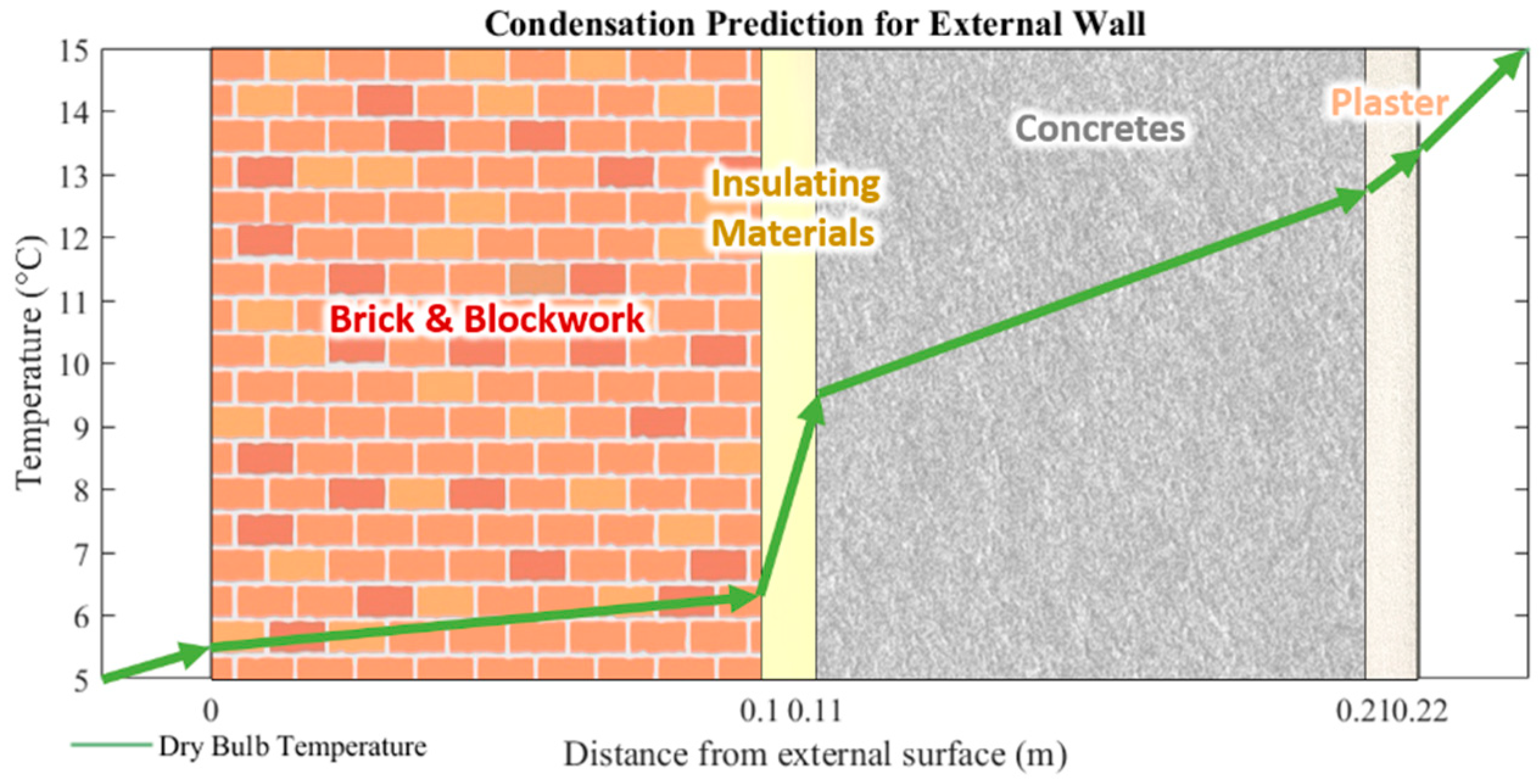
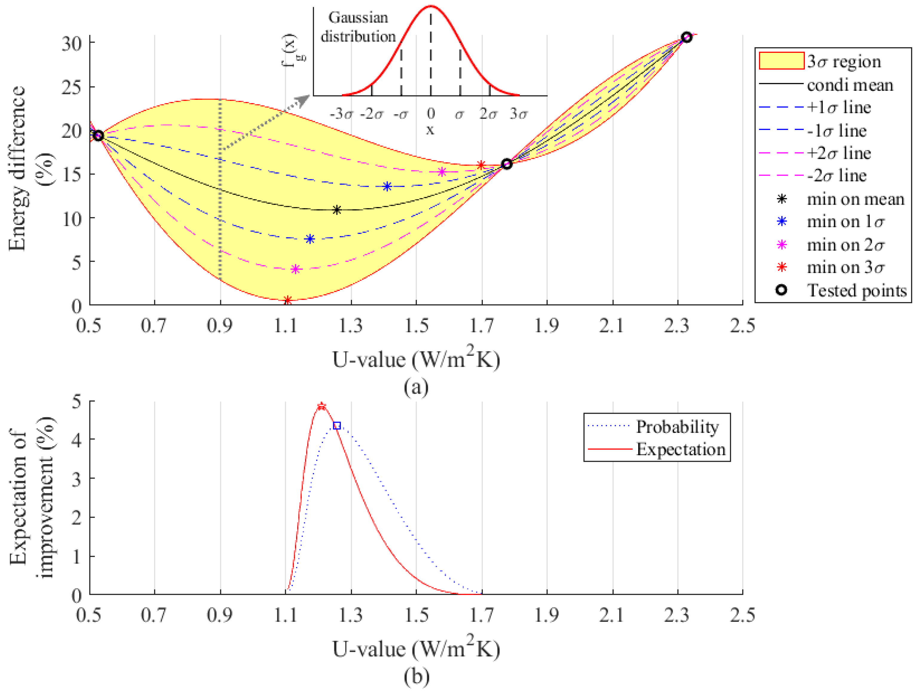
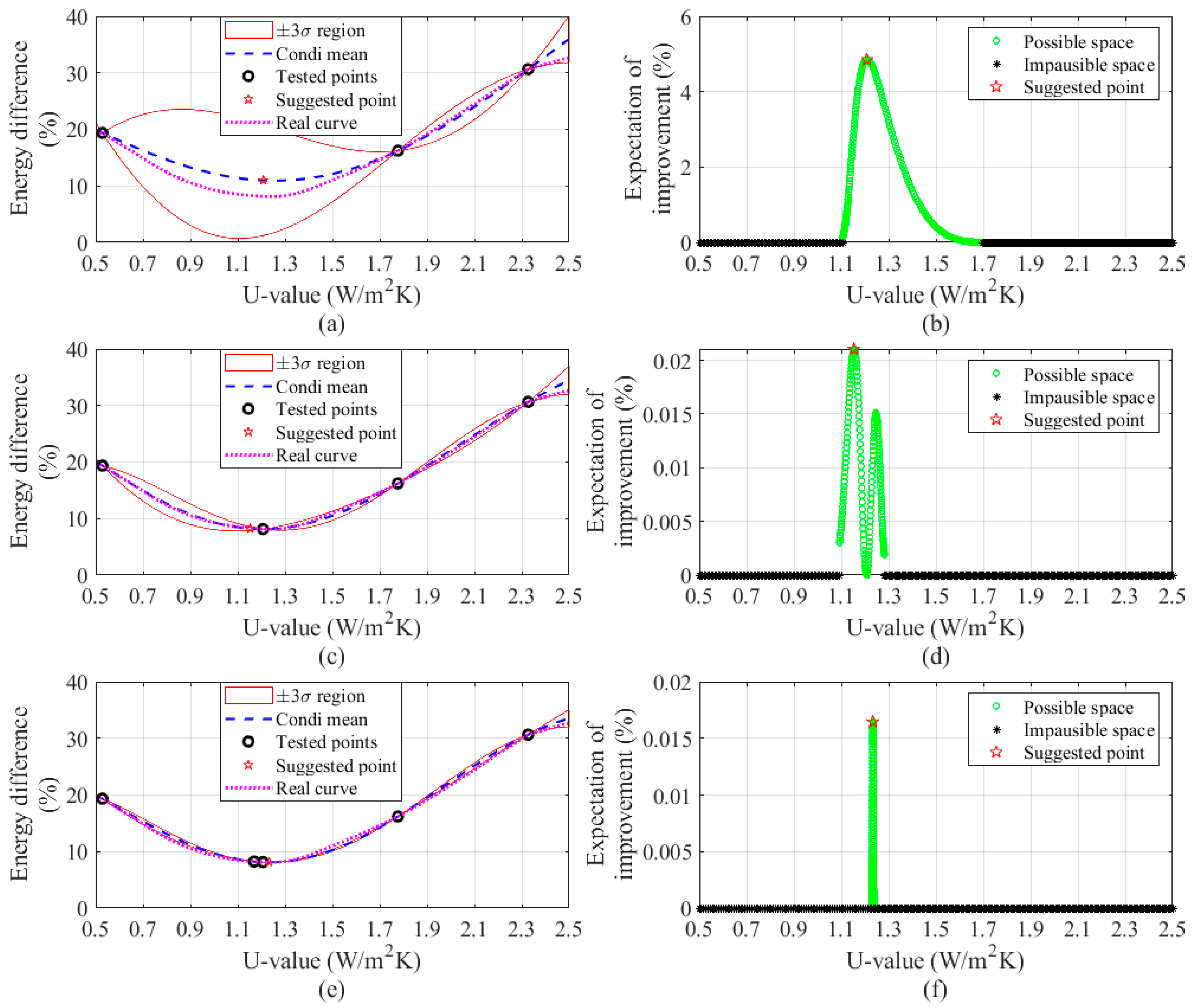
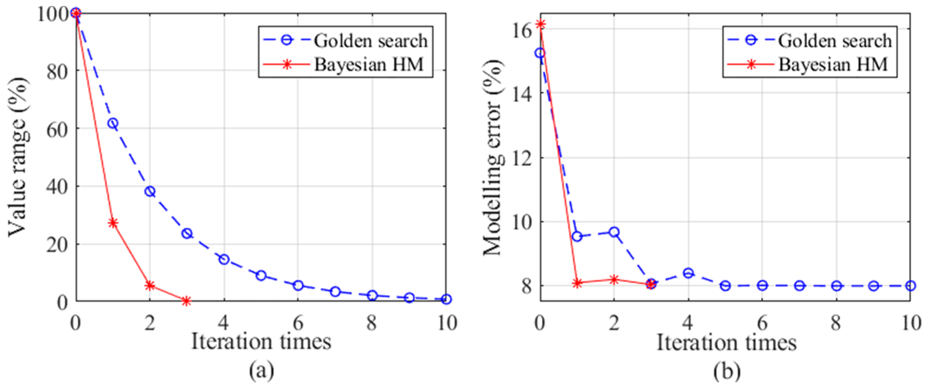
4.1. Wall Heat Resistance Coefficient Calibration

The thermal behaviour of external wall is one of the most significant factors of building envelope, which affects the heat demand for a given input weather profile. Thus, in the first case, the thermal transmittance coefficient, or U-value, of the external wall is chosen as the only thermal parameter to be calibrated. The error criteria for calibration are the relative RMS error of monthly heat demand, based on hourly prediction results and the recorded heat demand data (derived from the gas consumption). However, the hourly recorded heat consumption includes the uncertainty of human activities, which is known as disturbance to the heat demand affected by weather conditions. In order to reduce their impact, the calibration uses the data of monthly heat demand to calculate the prediction error. Then their relative RMS error can be obtained as ration of the RMS error (i.e., the difference between the simulated results with the recorded data) and the recorded monthly heat demand. The prediction error is finally known as the percentage error of predicted monthly heat demand to the real value.
In the building consumed energy calibration, the conditional mean and variance are calculated from the emulator based on the training from the tested points, as shown in Figure 4a. The black circles indicate the difference of heat demand between recorded data and simulated result at the tested U-value of the external wall in IES-VE simulation. Based on the initial tests, the point that causes the minimum heat demand difference needs to be obtained.
In the Gaussian distribution, its probability value at different variance is given as an explanation of the emulator’s process. In Figure 4a, the σ indicates the standard deviation, which is the square root of the variance. As the ‘three-sigma rule’ described, the points beyond the ±3σ limit are assumed as a small probability event and can be neglected, as seen in the Gaussian distribution. The yellow region is the 3σ region at the untested points to cover all the probability of the event. As the case is to find the point with the lowest energy difference, only the bottom differences are considered in the calculation. The black line shows the curve of conditional mean at untested points and indicates the expectation with the highest probability. The dashed blue line shows the lower probable curve of ±1σ away from the conditional mean line, while the dashed red line shows that of ±2σ. The star points show the min value of each line at ±1σ, ±2σ, and ±3σ. These can be used to emulate the expected global minimum point.
The probability density function (PDF) of the event that the minimum points match the real history data is shown as the blue dash line in Figure 4b. The wall U-value below the lowest value and above the highest value of the curve is deemed to the implausible points, whose expectation improvement is negative, or its probability of available improvement is too small. If only the highest probability is considered, it is too conservative in choosing the suggested point for the next iteration, and that will cause many more iteration steps. Therefore, in consideration of the benefit of energy difference reduction. The probability and expectation curves are shown in the red line in Figure 4b. The probability curve is calculated from its variance in Gaussian distribution, while the expectation curve is the product of probability and improvements. The red pentagram is not the highest probability point but is expected to get the best benefit.
Depending on the output of the emulator, the x value of the suggested point can be used as the next input for simulator testing. Figure 5 shows the calibration process in three iterations. The green area on the right side indicates the expected input space of the wall U-value. The initial parameter range of wall U-value is chosen from 0.5 W/m2K to 2.5 W/m2K, which covers most building types. The three initial tested points are randomly chosen from the original parameter ranges and tested in the simulator to get the result of energy difference to recorded data. In the figure, when the U value of external wall is 2.32 W/m2K the simulated heat demand is 32% different from that of the recorded data, which means the wall heat resistance coefficient is too high. In the same way, when the wall U-value is 0.52 and 1.78 W/m2K, the heat demand differences are 20% and 16%, respectively. In the first iteration, the potential input space is within the range of 1.1 W/m2K to 1.7 W/m2K as presented with the green line in Figure 5b, around 30% its initial input space. The first suggested parameter is at the wall U-value of 1.2 W/m2K with about 5% improvement in expectation. Then, IES-VE is used to simulate the building heat demand with the wall U-value at the suggested value.
The result is shown in the second iteration, with the new point of heat demand difference being less than 10% as in Figure 5c. Based on the information of the new tested point, the suggested parameter is updated to the wall U-value of 1.15 W/m2K, which is close to the last suggested point. The figure indicates that the emulator estimates the minimum point has higher probability within the range from 1.1 W/m2K to 1.28 W/m2K, approximate 9% of its initial input space. The suggested parameter at 1.15 W/m2K has the expectation of 20% improvement. The new suggested wall U-value is tested in the simulator for the next iteration. After the simulation test, it shows that the suggested U-value at 1.15 W/m2K was a bad guess with an even higher heat demand difference than the previous point. However, the new result updates the range of valid wall U-value from 1.21 W/m2K to 1.25 W/m2K, approximate 2% of its initial input space. The final suggested value of the wall U-value is 1.24 W/m2K. Thus, when the most expected improvement of the suggested point is less than the threshold, for example, 0.02% in this case, it is assumed that no more iteration is required. After the stopping criteria are met, the calibration gives the final range of the wall U-value to the building model. The calibration results of parameter range and simulation results of the suggested parameter in each iteration have been given in Table 2. The parameter range is reduced to 2%. With the calibrated parameter value, the prediction error of hourly heat demand is reduced from 16.1% to 8.11%, and the final suggested value of wall U-value is 1.24 W/m2K. The calibrated wall U-value is higher than in modern domestic buildings. The latest Scottish building regulations standards require a maximum U-value of 0.27 W/m2K for walls of new buildings [42]. Most buildings in the campus were constructed before the 1950s, before such regulations were introduced. The cavity of building external wall was left un-insulated and historical buildings were constructed with solid walls, which have even worse thermal resistance coefficient.
There are many optimisation methods for searching for the global minimum. However, most of the methods require the information of gradient or even second-order derivatives at tested point, such as the Gradient Descent and Newton’s method. In the present case study, the gradient at tested point is not available from the physics-based energy model. Thus, to make a meaningful comparison, the proposed calibration method is compared with the golden search algorithm that does not require gradient information. The comparison is shown in Figure 6a, the BHM method only needs four iteration times to reduce the initial parameter ranges into less than 2% while the golden search method needs ten iteration times to reduce the parameter ranges, showing that the proposed method only needs much fewer iteration times to run the simulation in calibrating a model parameter. The comparison of modelling error between golden search and BHM method after each iteration is given in Figure 6b. Although both methods find the point of least modelling error before the final iteration, the wide range of possible parameter space also needs to be reduced to provide enough evidence. The BHM not only obtains a much faster speed in finding the optimised point, but also solves the issue that the Golden search method will reduce the search speed when it gets close to the target point. The improved efficiency of the approach increases the calibration speed and reduces the computational cost to run the large simulation model of a district-level heating network with multiple buildings.

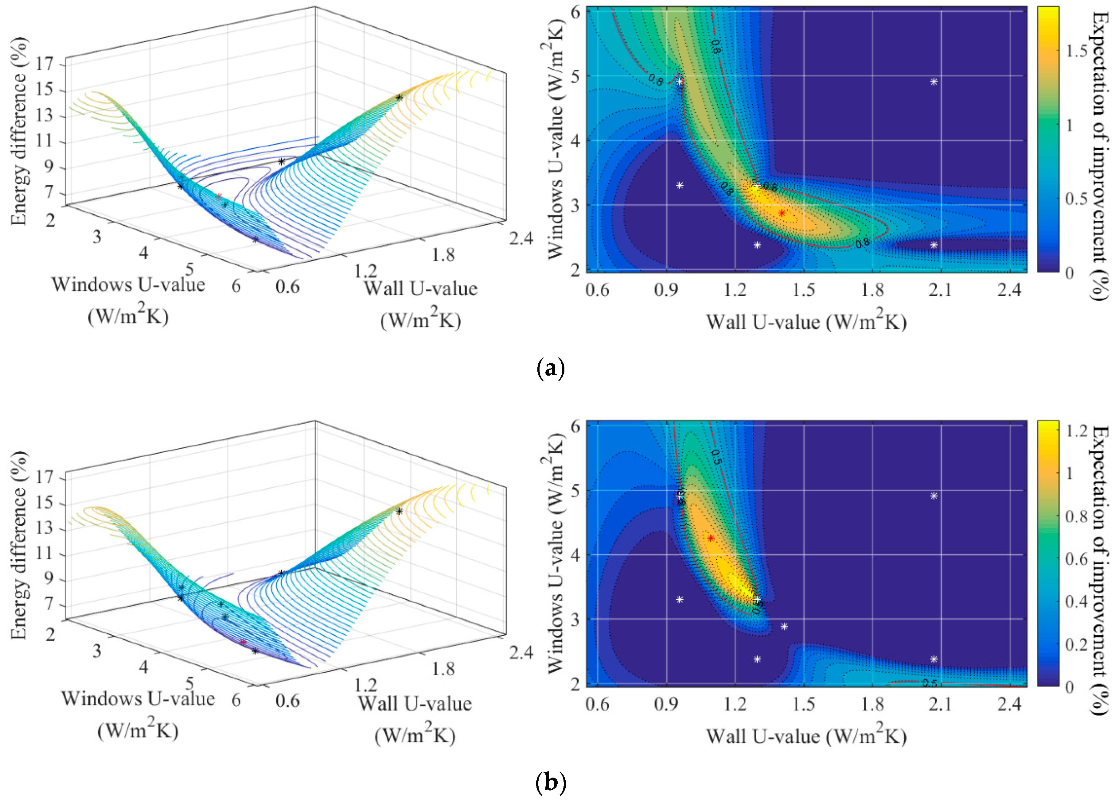
4.2. Dual-Parameters Calibration

Apart from the external wall, the thermal transmittance coefficient of windows is also a significant parameter in the building heat transfer. The windows’ U-value depends on its thickness, cavity and types, such as single or double-glazed window. The parameters of windows’ thermal behaviour should also consider the average human activities to windows, such as opening a window that reduces the total thermal resistance of the building envelope. If the U-value of external wall and windows are calibrated individually using the single parameter calibration approach, it could not calculate their internal interaction between the parameters, and the calibration processes have to be operated many times. Therefore, an approach of calibrating dual parameters using BHM approach can be implemented. The results of calibrating both the wall U-value and windows U-value together are shown in Figure 7.
The left figure in Figure 7a shows the surface of the simulated error to the recorded data regarding the variation of the two calibration parameters. The figures on the right show the likelihood density function that indicates the expectation of improvement at each point. From the colour bar, the lighter area shows higher likelihood while darker area shows the lower probability. The density map indicates the expected parameter input area to be calibrated in the two-parameter map. In the first iteration, the parameter input space has been reduced to 19% of its initial range; while in the second and third iterations, the input space has been reduced to 10% and 4%, respectively, as seen in Figure 7b,c. After several iterations, the final range of both parameters can be detected from the calibration. The wall U-value is calibrated to the range between 1.05 W/m2K and 1.2 W/m2K, and the windows U-value is calibrated to the range between 3.7 W/m2K to 4.8 W/m2K. The final simulated error is reduced to about 6.2% compared with the recorded heat demand.

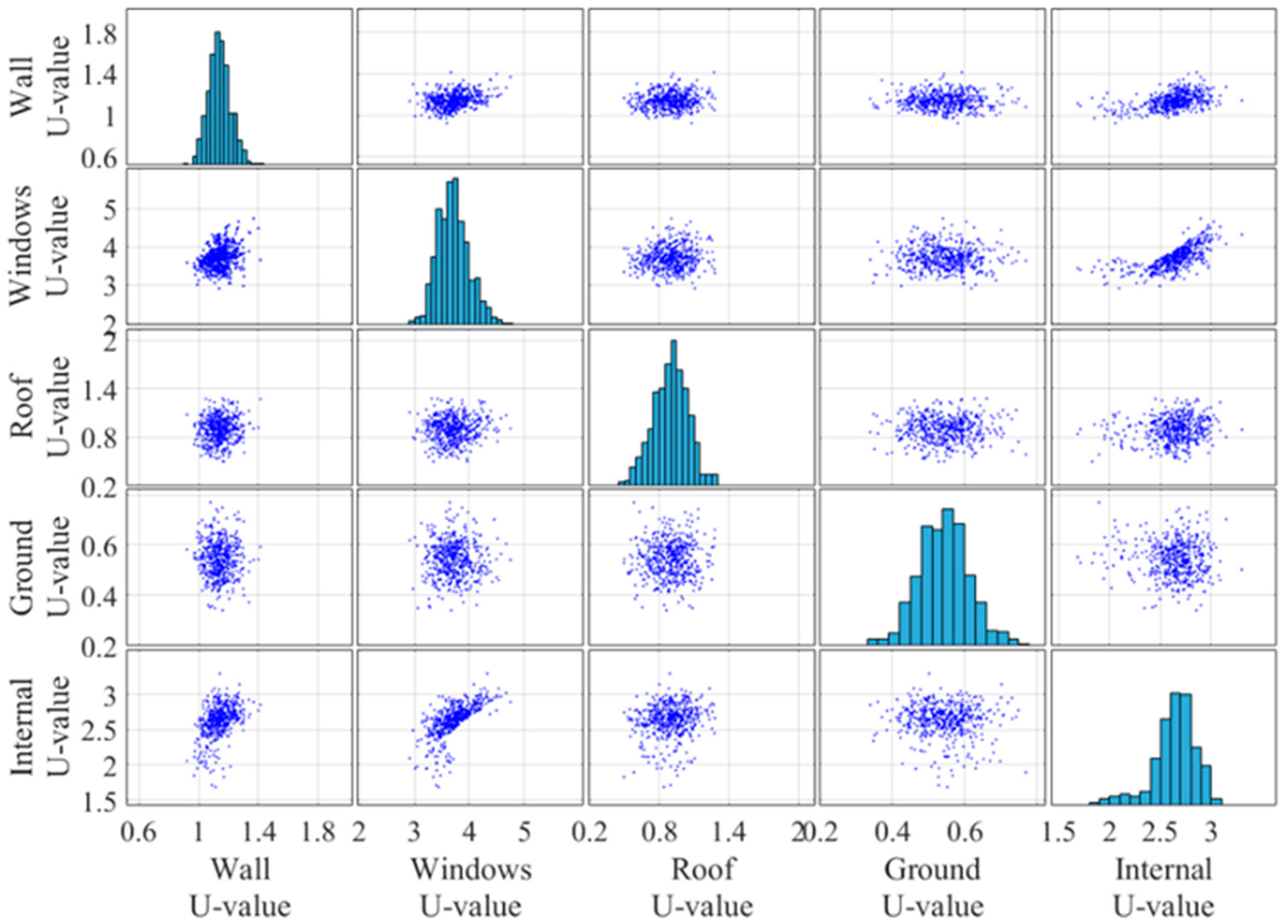
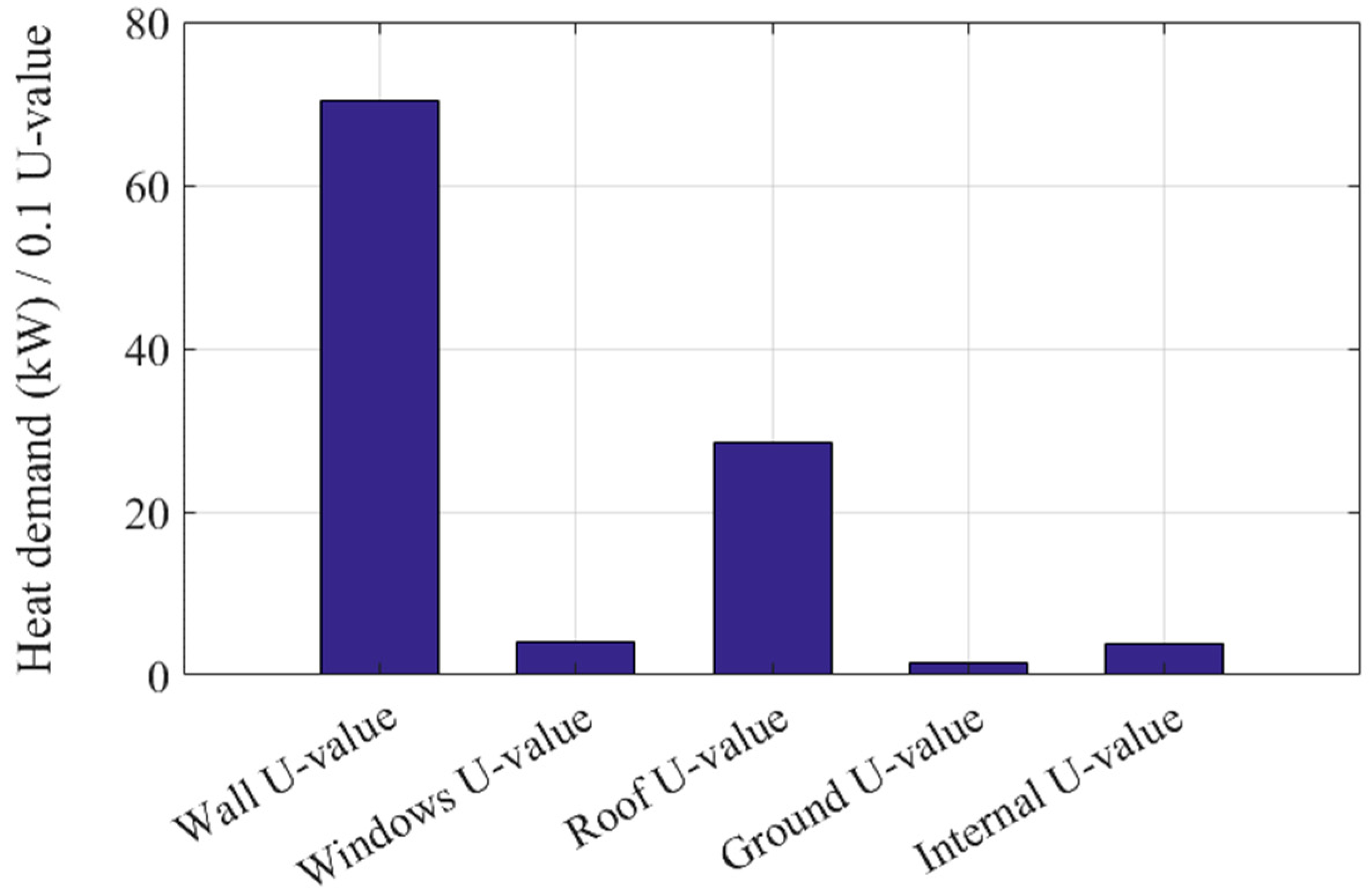
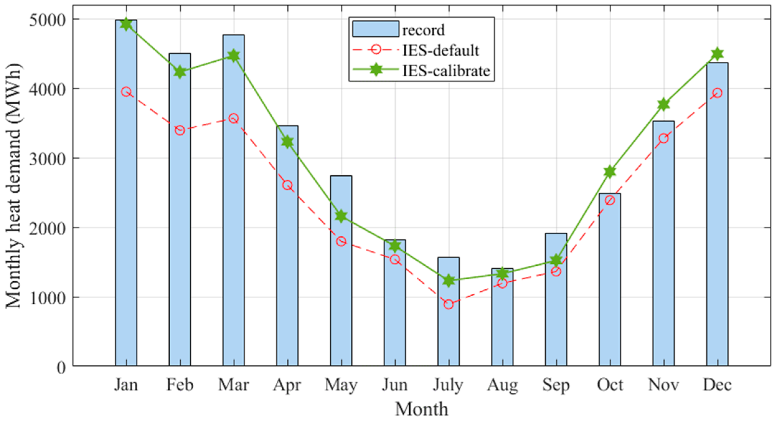
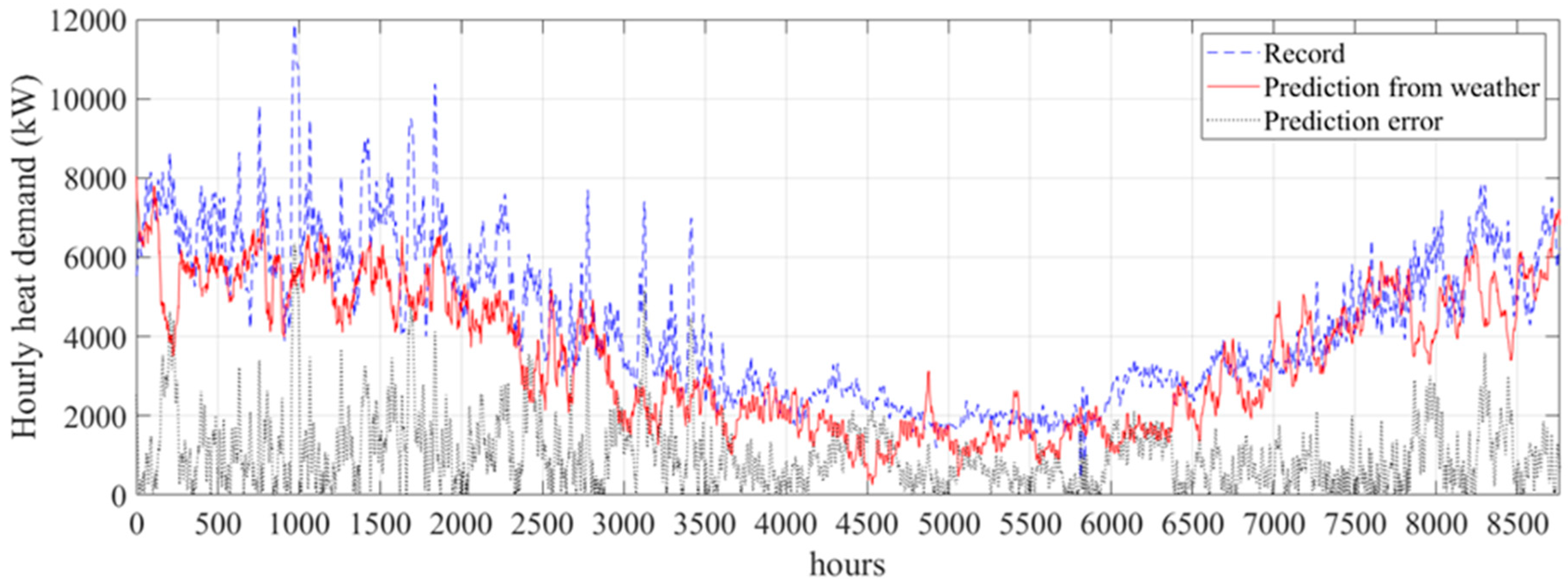
4.3. Multi-Parameters Calibration

In addition to external wall U-value and windows U-value, several more parameters affect the total energy consumption in building models. In the next case, three additional parameters, the U-value of roof, ground, and internal partition/floor/ceiling, will be calibrated simultaneously for the building model. These five parameters describe the building fabrication and thermal behaviour of all buildings, and they are calibrated together with random values as initially tested points to feed the emulator for the expected value at the untested points. The number of untested points grows exponentially with the number of calibration parameters. To reduce the computational burden of the emulator to calculate the conditional expectation and variance at untested points, the sampling method is used to randomly choose the points from the prior distribution range as untested points.
Based on the calculated value from the emulator, the points with expectation higher than the threshold are retained in the result while the points with lower expectation are reduced from the initial range. Only the points from the remaining range will be considered as the untested points. The points beyond the remaining range are considered as implausible. Due to the high-dimension results of five parameters, the scatter matrix plot is given to compare the parameters in pairs, as seen in Figure 8.
In the figure, each row and column show the remaining points of the corresponding parameter regarding the other four parameters. For example, the second plot in the first column indicates the remaining points whose parameters are chosen with the corresponding external wall U-value and windows U-value. The same points with corresponding external wall U-value and roof U-value are given in the third plot in the first column, and so were other plots. The bar charts on the diagonal line show the statistical distribution of each parameter. The first figure in the first column indicates the statistic result of all the remaining points distributed along with the parameters of the external wall. After several iterations in the multi-parameter calibration process, the maximum likelihood distribution of external wall U-value is from 1.05 W/m2K to 1.25 W/m2K after the final iteration of multi-parameter calibration. Based on the statistical distribution result of each parameter, the best parameter values can be chosen from the highest expected range from the calibration results. The remaining space of each parameter is the maximum likelihood range to make the model output fit the recorded heat demand. The simulation results show that the monthly and hourly prediction error has been reduced to 4.3% and 12.63%, respectively, compared with the recorded data. The calibrated parameters and their suggested results are shown in Table 3.
To validate the effect of model parameters, the sensitivity analysis has been made to provide the elementary effect of each parameter. The Morris method, which is the most commonly used global sensitivity analysis method, has been used to test the elementary effect in the case [43]. The basic idea of Morris method is to evaluate the response of model output on the basis of a small change in a single parameter. The mean elementary effect of a single parameter is presented as:
μ i * = 1 R j = 1 R | f ( x 1 , , x i + Δ , , x n ) f ( x 1 , , x n ) Δ |
where μ i * is the mean elementary effect of the ith parameter out of n parameters in total, j is the number of tested data out of R tested data in total; Δ is a small change in parameter and f ( · ) indicates the model output with related parameters.
The results of the sensitivity analysis are shown in Figure 9. The x-axis shows five parameters of the walls, windows, roof, ground and internal partition. The y-axis indicates the elementary effect with the unit of kW per change of U value in every 0.1 W/m2K. From the result, the wall U value has the highest elementary effect with about 70 kW increase of heat demand in every increment of 0.1 W/m2K in its U value. The second most significant parameter for the building thermal resistance is the roof U-value followed by that of windows and internal partitions. The ground U-value is the least significant parameter that affects the building thermal resistance and heat demand.
The calibrated result of the IES-VE model is compared with the recorded data and default result before calibration as given in Figure 10. The results show that the calibrated monthly heat demand has reduced from 16.3% to 4.3% as the best calibration result.
After the most probable parameters chosen after the calibration from the monthly result, the hourly heat demand of each building can be predicted from the model. The result comparison among one parameter calibration, two parameters calibration, and multi parameters calibration is given in Table 4. In the one parameter calibration, only the wall thickness has been calibrated and results in the smallest range. The result of that in the two-parameter calibration covers the same range. Because the second parameter has been calibrated together, the final range of the wall thickness is wider than that of the single parameter calibration. The same situation has been found in the multi-parameter calibration as well. The final range of each parameter is wider than that of the single parameter calibration, but the prediction error of model simulation is less in multi-parameter calibrations.
The average prediction error of hourly heat demand after multi-parameter calibration is around 12.6%. That means the prediction accuracy of using the proposed approach is more than 87% in predicting the hourly heat demand without known the detailed building information. The overall waveform of the predicted heat demand matches the recorded data and can be used for prediction of the whole heating network. In practical, the real building energy consumption not only depends on these parameters and weather conditions but also the human activities and other uncertainties, such as the observation error from the sensor, model uncertainty in simulating the thermal behaviour. In fact, the uncertainties, such as the domestic hot water usage and internal gains, are also contributors of heat demand, but they are hard to predict as it highly depends on the activities of occupants. In the IESVE simulation, the domestic hot water usage and internal gains have been set as a constant ratio of the total heat demand of each building. The model only predicts heat demand affected by the weather conditions (which is the dominant factor) in this work. The variation of heat demand caused by those secondary factors such as human activities is beyond the scope of this work, and it can be addressed by building control system.
The hourly heat demand prediction is shown in Figure 11. The recorded data of hourly heat demand is shown by the blue line. The red line represents the prediction on the basis of weather profile only, of which the actual human activities within the buildings have not been properly considered in the model. The grey line shows the absolute difference between these two sets of data, namely the prediction error of the model basis on weather profile. In comparison with Figure 10, one can find that the hourly prediction has much higher error than the monthly prediction.
There are two points should be highlighted here: (1) The IES-VE model has some default settings of human activities when the type of building is selected. However, such settings are just a constant value (i.e., an extra percentage of heat demand), which are very different from actual user’s behaviour that however are dynamic and have not been recorded by the University’s energy centre. Hence, the prediction error can be largely attributed to the unknown human activities within the buildings. (2) The model itself does not forecast weather, but uses the hourly weather profile of a whole year embedded in the IES-VE software, which are historical weather data recorded by the weather centre at Glasgow Airport. For this reason, the uncertainty introduced by the weather profile is considered negligible, and thus neglected in this paper. Furthermore, the hourly weather profile is used, the prediction is can be considered as one hour ahead of time.
Comparing Figure 10 with Figure 11, with reference to Table 4, one can find that the hourly prediction result has much higher error than the monthly prediction result, showing that the accuracy of the model is strongly affected by human activities, especially at short time scale. In general, the more factors being considered, the more accurately the model can predict the heating demand. Since not all input parameters can be accurately measured (e.g., user’s behaviour), the calibration methods developed in this paper becomes necessary and useful.
In summary, the proposed approach uses IES-VE to build the bottom-up model of a district-level heating network, and some unknown parameters are calibrated using the Bayesian-based approach to improve the model’s accuracy. The model can predict the hourly heating demand of each building with the error less than 13% for a case study, of which a number of building parameters are unknown.

5. Conclusions

This paper developed an approach to predict the hourly heat demand of a district-level heating network, using a model calibrated by the proposed Bayesian-based calibration method and monthly recorded data. The IES-VE building energy software is used to build the bottom-up model of buildings in a DHN. Due to the lack of detailed building parameters and heavy computational load of simulating such a large model, a Bayesian history matching based calibration method was proposed to calibrate the model over a shorter time span without the requirement of gradient calculation. In the approach, a statistical method-based emulator has been designed to estimate the conditional expectation and variance of model mismatch at untested points for the calibration iterations. The designed emulator-based calibration method has been compared with a traditional golden search algorithm, and the results show that the Bayesian approach-based emulator performs better with fewer calibration times to find the optimal point. Another case study has been designed to validate the proposed method in calibrating the single parameter, two-parameters, and multi-parameters of building envelope. The results indicate that the method is reliable and efficient to calibrate thermal parameters in building energy models. The multi-parameters calibration gives better performance by calibrating all parameters simultaneously. Finally, it is verified that the proposed approach can predict the hourly heat demand of a DHN without the requirements of detailed building information and accurate recorded data.

Author Contributions

Conceptualization: S.C., D.F. and Z.Y.; Methodology: S.C.; Software: S.C.; Formal Analysis: S.C.; Investigation: S.C.; Resources: S.C., Z.Y. and D.F.; Data Curation: S.C.; Writing—Original Draft Preparation: S.C.; Writing—Review & Editing: S.C., D.F., Z.Y., J.Y.; Visualization: S.C.; Supervision: Z.Y., D.F. and J.Y.; Project Administration: Z.Y.; Funding Acquisition: Z.Y.

Funding

This research was funded by Energy Technology Partnership (ETP) and SP Distribution PLC (Scottish Power), grant number 146. And the APC was funded by Energy Technology Partnership and Scottish Power.

Acknowledgments

The research presented in this article was undertaken as part of a project joint founded by Energy Technology Partnership (ETP), SP Distribution PLC (Scottish Power). The authors would like to thank Gillian Brown for providing valuable information on the campus energy consumption.

Conflicts of Interest

The authors declare no conflict of interest. The sponsors had no role in the design, execution, interpretation, or writing of the study.

References

  1. Heo, Y.; Choudhary, R.; Augenbroe, G. Calibration of building energy models for retrofit analysis under uncertainty. Energy Build. 2012, 47, 550–560. [Google Scholar] [CrossRef]
  2. Lund, H.; Andersen, A.N.; Østergaard, P.A.; Mathiesen, B.V.; Connolly, D. From electricity smart grids to smart energy systems—A market operation based approach and understanding. Energy 2012, 42, 96–102. [Google Scholar] [CrossRef]
  3. Kienzle, F.; Favre-Perrod, P.; Arnold, M.; Andersson, G. Multi-energy delivery infrastructures for the future. In Proceedings of the 2008 First International Conference on Infrastructure Systems and Services: Building Networks for a Brighter Future (INFRA), Rotterdam, The Netherlands, 10–12 November 2008. [Google Scholar]
  4. Wu, F.; Guo, Q.; Sun, H.; Pan, Z. Research on the optimization of combined heat and power microgrids with renewable energy. In Proceedings of the 2014 IEEE PES Asia-Pacific Power and Energy Engineering Conference (APPEEC), Hong Kong, China, 7–10 December 2014. [Google Scholar]
  5. Ozkahraman, H.T.; Bolatturk, A. The use of tuff stone cladding in buildings for energy conservation. Constr. Build. Mater. 2006, 20, 435–440. [Google Scholar] [CrossRef]
  6. Cøengel, Y. Heat and Mass Transfer: A Practical Approach; McGraw-Hill: New York, NY, USA, 2007. [Google Scholar]
  7. Fan, C.; Wang, J.; Gang, W.; Li, S. Assessment of deep recurrent neural network-based strategies for short-term building energy predictions. Appl. Energy 2019, 236, 700–710. [Google Scholar] [CrossRef]
  8. Bacher, P.; Madsen, H. Identifying suitable models for the heat dynamics of buildings. Energy Build. 2011, 43, 1511–1522. [Google Scholar] [CrossRef] [Green Version]
  9. Heo, Y.; Augenbroe, G.; Graziano, D.; Muehleisen, R.T.; Guzowski, L. Scalable methodology for large scale building energy improvement: Relevance of calibration in model-based retrofit analysis. Build. Environ. 2015, 87, 342–350. [Google Scholar] [CrossRef] [Green Version]
  10. Balaji, N.; Mani, M.; Reddy, B.V. Dynamic thermal performance of conventional and alternative building wall envelopes. J. Build. Eng. 2019, 21, 373–395. [Google Scholar] [CrossRef]
  11. Reddy, T.A. Literature Review on Calibration of Building Energy Simulation Programs: Uses, Problems, Procedures, Uncertainty, and Tools. ASHRAE Trans. 2006, 112, 226–240. [Google Scholar]
  12. Royapoor, M.; Roskilly, T. Building model calibration using energy and environmental data. Energy Build. 2015, 94, 109–120. [Google Scholar] [CrossRef] [Green Version]
  13. Raftery, P.; Keane, M.; O’Donnell, J. Calibrating whole building energy models: An evidence-based methodology. Energy Build. 2011, 43, 2356–2364. [Google Scholar] [CrossRef]
  14. Raftery, P.; Keane, M.; Costa, A. Calibrating whole building energy models: Detailed case study using hourly measured data. Energy Build. 2011, 43, 3666–3679. [Google Scholar] [CrossRef]
  15. Soebarto, V.I. Calibration of hourly energy simulations using hourly monitored data and monthly utility records for two case study buildings. In Proceedings of the Building Simulation, 5th International IBPSA Conference, Prague, Czech Republic, 8–10 September 1997. [Google Scholar]
  16. Bertagnolio, S. Evidence-Based Model Calibration for Efficient Building Energy Services. Ph.D. Thesis, Université de Liège, Liège, Belgium, 2012. [Google Scholar]
  17. Yang, Z.; Becerik-Gerber, B. A model calibration framework for simultaneous multi-level building energy simulation. Appl. Energy 2015, 149, 415–431. [Google Scholar] [CrossRef]
  18. Ruiz, G.R.; Bandera, C.F.; Temes, T.G.; Gutierrez, A.S. Genetic algorithm for building envelope calibration. Appl. Energy 2016, 168, 691–705. [Google Scholar] [CrossRef]
  19. Struck, C.; Hensen, J.; Kotek, P. On the application of uncertainty and sensitivity analysis with abstract building performance simulation tools. J. Build. Phys. 2009, 33, 5–27. [Google Scholar] [CrossRef]
  20. Eisenhower, B.; O’Neill, Z.; Fonoberov, V.; Mezic, I. Uncertainty and sensitivity decomposition of building energy models. J. Build. Perform. Simul. 2012, 5, 171–184. [Google Scholar] [CrossRef]
  21. Tindale, A. Third-order lumped-parameter simulation method. Build. Serv. Eng. Res. Technol. 1993, 14, 87–97. [Google Scholar] [CrossRef]
  22. Underwood, C. An improved lumped parameter method for building thermal modelling. Energy Build. 2014, 79, 191–201. [Google Scholar] [CrossRef] [Green Version]
  23. Aksoezen, M.; Daniel, M.; Hassler, U.; Kohler, N. Building age as an indicator for energy consumption. Energy Build. 2015, 87, 74–86. [Google Scholar] [CrossRef]
  24. Walker, R.; Pavía, S. Thermal performance of a selection of insulation materials suitable for historic buildings. Build. Environ. 2015, 94, 155–165. [Google Scholar] [CrossRef]
  25. Mustafaraj, G.; Marini, D.; Costa, A.; Keane, M. Model calibration for building energy efficiency simulation. Appl. Energy 2014, 130, 72–85. [Google Scholar] [CrossRef]
  26. Yang, S.; Pilet, T.; Ordonez, J. Volume element model for 3D dynamic building thermal modeling and simulation. Energy 2018, 148, 642–661. [Google Scholar] [CrossRef]
  27. Yuan, J.; Nian, V.; Su, B. A Meta Model Based Bayesian Approach for Building Energy Models Calibration. Energy Procedia 2017, 143, 161–166. [Google Scholar] [CrossRef]
  28. Yuan, J.; Nian, V.; Su, B.; Meng, Q. A simultaneous calibration and parameter ranking method for building energy models. Appl. Energy 2017, 206, 657–666. [Google Scholar] [CrossRef]
  29. Gao, H.; Koch, C.; Wu, Y. Building information modelling based building energy modelling: A review. Appl. Energy 2019, 238, 320–343. [Google Scholar] [CrossRef]
  30. Baker, P. U-Values and Traditional Buildings; Historic Scotland Conservation Group: Glasgow, UK, 2011. [Google Scholar]
  31. Balaji, N.; Mani, M.; Reddy, B.V. Discerning heat transfer in building materials. Energy Procedia 2014, 54, 654–668. [Google Scholar] [CrossRef]
  32. Evangelisti, L.; Guattari, C.; Gori, P.; Bianchi, F. Heat transfer study of external convective and radiative coefficients for building applications. Energy Build. 2017, 151, 429–438. [Google Scholar] [CrossRef]
  33. Masatin, V.; Latõšev, E.; Volkova, A. Evaluation factor for district heating network heat loss with respect to network geometry. Energy Procedia 2016, 95, 279–285. [Google Scholar] [CrossRef]
  34. Ullah, T.; Healy, W.M. The Effect of Piping Heat Losses on the Efficiency of Solar Thermal Water Heating in a Net-Zero Energy Home. In Proceedings of the 2015 ASHRAE Winter Conference, Chicago, IL, USA, 24–28 January 2015. [Google Scholar]
  35. Yan, D.; Zhe, T.; Yong, W.; Neng, Z. Achievements and suggestions of heat metering and energy efficiency retrofit for existing residential buildings in northern heating regions of China. Energy Policy 2011, 39, 4675–4682. [Google Scholar] [CrossRef]
  36. Vesterlund, M.; Sandberg, J.; Lindblom, B.; Dahl, J. Evaluation of losses in district heating system, a case study. In Proceedings of the International Conference on Efficiency, Cost, Optimization, Simulation and Environmental Impact of Energy Systems (ECOS 2013), Guilin, China, 16–19 July 2013. [Google Scholar]
  37. Bayarri, M.J.; Berger, J.O.; Paulo, R.; Sacks, J.; Cafeo, J.A.; Cavendish, J.; Lin, C.H.; Tu, J. A framework for validation of computer models. Technometrics 2007, 49, 138–154. [Google Scholar] [CrossRef]
  38. Kennedy, M.C.; O’Hagan, A. Bayesian calibration of computer models. J. R. Stat. Soc. Ser. B (Stat. Methodol.) 2001, 63, 425–464. [Google Scholar] [CrossRef]
  39. Robert, C.; Casella, G. Monte Carlo Statistical Methods; Springer Science & Business Media: Berlin/Heidelberg, Germany, 2013. [Google Scholar]
  40. Andrianakis, I.; Vernon, I.R.; McCreesh, N.; McKinley, T.J.; Oakley, J.E.; Nsubuga, R.N.; Goldstein, M.; White, R.G. Bayesian history matching of complex infectious disease models using emulation: A tutorial and a case study on HIV in Uganda. PLoS Comput. Biol. 2015, 11, e1003968. [Google Scholar] [CrossRef] [PubMed]
  41. Rasmussen, C.E. Gaussian processes in machine learning. In Summer School on Machine Learning; Springer: Berlin/Heidelberg, Germany, 2003. [Google Scholar]
  42. Scottish Government. Building Standards Technical Handbook 2019: Non-Domestic Buildings; Scottish Government: Edinburgh, UK, 2019.
  43. Campolongo, F.; Cariboni, J.; Saltelli, A. An effective screening design for sensitivity analysis of large models. Environ. Model. Software 2007, 22, 1509–1518. [Google Scholar] [CrossRef]
Figure 1. (a) The 3D satellite image obtained from Google global; (b) bottom-up model of buildings in a heating network built in SketchUp.
Energies 12 03408 g001
Figure 2. Temperature and condensation prediction for external building wall in IES.
Energies 12 03408 g002
Figure 3. Flow chart of history matching calibration approach.
Energies 12 03408 g003
Figure 4. The process of emulator for model parameter calibration. (a) Emulator’s process with Gaussian distribution; (b) the probability density function and expectation of improvement.
Energies 12 03408 g004
Figure 5. Results of one parameter calibration after each iteration. (a) Emulator’s result in the 1st iteration; (b) expected input space and suggested result in the 1st iteration; (c) emulator’s result in the 2nd iteration; (d) expected input space and suggested result in the 2nd iteration; (e) emulator’s result in the 3rd iteration; (f) expected input space and suggested result in the 3rd iteration.
Energies 12 03408 g005
Figure 6. Comparison of BHM calibration method with traditional golden search method. (a) The reduction of value range; (b) the reduction of modelling error.
Energies 12 03408 g006
Figure 7. Two parameters calibration result after (a) the first iteration, (b) the second iterations and (c) the third iterations.
Energies 12 03408 g007aEnergies 12 03408 g007b
Figure 8. The remaining sample points projected to the corresponding parameters of external wall, windows, roof, ground, and internal partition.
Energies 12 03408 g008
Figure 9. Elementary effect sensitivity analysis of each calibrated parameter.
Energies 12 03408 g009
Figure 10. Prediction result using IES-VE comparing with recorded monthly heat demand.
Energies 12 03408 g010
Figure 11. Comparison between record and predicted hourly heat demand.
Energies 12 03408 g011
Table 1. Settings of other parameters in IES-VE model.
ParametersValue & Unit
Room heating set-point21.8 °C
Natural ventilation in air exchangel/people/m2
Occupant density of people2 m2/people
Internal gains of people90 W/people
Lighting and equipment power density45 W/m2
Table 2. Calibration results of each iteration in single parameter calibration.
ParametersIterationCalibrated Range (W/m2K)Range to Its Initial (%)Suggested Value (W/m2K)Prediction Error (%)
External wall U-value (W/m2K)0th0.5–2.51001.7516.24
1st1.1–1.728.21.28.16
2nd1.1–1.289.11.158.27
3rd1.21–1.251.91.248.11
Table 3. Calibrated parameters with initial range and calibrated value.
ParametersUnitInitial RangeCalibrated RangeRange to Its Initial (%)Suggested Value
Wall U-valueW/m2K0.5–2.51.05–1.25101.16
Windows U-valueW/m2K2–63.2–4.2253.8
Roof U-valueW/m2K0.2–2.20.6–1.1250.95
Ground U-valueW/m2K0.2–0.90.4–0.7430.55
Internal U-valueW/m2K1.5–3.62.4–3292.7
Table 4. Prediction result comparison among different number of parameters to be calibrated.
ParametersMonthly Prediction ErrorHourly Prediction Error
Before calibration16.3%18.5%
One parameter calibration8.02%15.4%
Two parameters calibration6.1%13.2%
Multi parameters calibration4.3%12.6%

