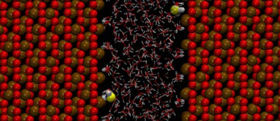
We also limit ourselves to some of the important hydrate phase transitions involved in hydrate formation in porous media. Formation of hydrate on the interface between a separate phase containing hydrate formers, and hydrate formation towards mineral surfaces, are the two fastest routes. When these two routes have created a hydrate film there will also be some hydrate formation from dissolved hydrate former in water. For methane this is limited by fairly low solubility, while the higher solubility of CO2 in water makes this route far more significant.
In order for a hydrate particle to reach critical size, the hydrate former molecules must be transported from an outer boundary on the liquid water side and through an interface layer of gradually increased water structure. The more structured the water, the slower the transport. The necessary time for enough hydrate former molecules to reach surface of the hydrate core at critical size is the nucleation time. Further growth through the hydrate film is very slow as indicated above. Since heat transport is very fast, and maybe two to three orders of magnitude faster than mass transport in liquid water, it will be several orders of magnitude faster than mass transport through hydrate. Assuming a constant mass transport rate through the hydrate film in order to supply the hydrate film with hydrate formers we are then able to estimate hydrate film thickness as a function of time. This will provide a basis for evaluating the necessary dynamics needed to break hydrate films, and correspondingly ensure that measures can be taken to prevent blocking hydrate films.
2.1. Hydrate Formation from Water and a Separate Phase Containing Hydrate Formers
Hydrate phase transition along the equilibrium curve is reversible. At equilibrium the free energy changes of the hydrate formation from liquid water (or ice) and hydrate formers coming from gas, liquid or fluid state is zero. Outside of equilibrium the molar free energy change, as given by Equation (1) below, has to be negative.
The superscript H1 denotes this specific heterogeneous phase transition. T is temperature, P is pressure. x is mole-fraction in either liquid or hydrate (denoted with a superscript H). y is mole-fraction in gas (or liquid, or fluid) hydrate former phase; i is an index for hydrate formers. Superscript water denotes a water phase. Generally this is ice, liquid or adsorbed water on mineral surfaces. In this work we only consider liquid water; µ is chemical potential. x is mole-fraction in liquid water or hydrate (as given by superscripts). Vector sign denote mole-fractions of all components in the actual phase.
Symmetric excess formulation for liquid water chemical potential is given by:
when
xH2O approaches unity.
Water as superscript on the left-hand side distinguishes liquid water phase from water in the hydrate phase. A right-hand side approximation of Equation (2) is not necessary but good enough for the purpose of this work. The alternative would be to use a model for the activity coefficient or utilization of the Gibbs-Duhem relation. In our phase field theory (PFT) modelling of CO
2 hydrate phase transition dynamics studies [
14,
15] we used the latter approach. Our PFT models are fairly complex and a simpler kinetic model might be more useful in order to visualize the various stages of the hydrate formation.
Water chemical potential in the hydrate structure is given by [
16]:
H denotes hydrate and superscript
O on first term on right hand side denotes empty clathrate. Calculated values for water chemical potentials in empty hydrates of structure I and II are readily available from model water (TIP4P) simulations [
12] as discussed above. Cavities per water in structure I hydrate,
νk is 1/23 for small cavities and 3/23 for large cavities.
is the canonical partitition function for s guest of type
i in cavity type
k. For a rigid water lattice the result is a Boltzmann integral over all possible water-guest and guest-guest interactions and a function of the free energy of the huest molecule [
12]. This is the most common way to calculate
in various available codes for hydrate equilibrium. A different formulation of
utilize a perturbation approach in which the movements of the guest molecule, relative to energy minimum position in the cavity, is approximated by an harmonic oscillator. The advantage of this approach is that some frequencies of guest movements may interfere with the water lattice librational frequencies. As such we directly also get calculations for these effects, which are typically included as empirical correction, incorporated. For CO
2 a comparison with a rigid lattice calculations and the harmonic oscillator approach reveal a destabilization effect of 1 kJ/mole due to CO
2 movements in the large cavity of structure I [
12]:
β is the inverse of the universal gas constant times temperature.
μki is the chemical potential of guest molecule
i in hydrate cavity of type
k. At equilibrium this chemical potential is equal to the chemical potential for the same molecule in the phase it comes from during the hydrate formation. For Equation (1) that means gas, liquid or fluid as a separate phase. In a non-equilibrium situation the guest chemical potentials are adjusted for distances from equilibrium through a Taylor expansion, as discussed later. The free energies of inclusion (latter term in the exponent) are given in
Table 3 below.
Filling fractions in the various cavities, and mole-fractions in the hydrate are given by:
is the filling fraction of component
i in cavity type
k:
ν is fraction of cavity per water. Corresponding mole-fraction water is then given by:
The associated hydrate free energy is then:
where
µ is chemical potential.
H2O subscripts denote water.
i are hydrate formers.
H superscripts denote hydrate.
x is mole-fraction in hydrate (superscript
H) and
G is free energy.
Guest molecule i (in the case of this work either CO
2 or CH
4) chemical potential that enters Equations (4) and (8) at equilibrium is given by:
where
yi is the mole-fraction of component
i in the gas (or liquid or fluid) mixture.
is the fugacity coefficient for component
i. Chemical potential for a monoatomic model of methane in ideal gas state is trivial and analytical from statistical mechanics and the Boltzmann integral over translational momentums. For the rigid CO
2 model there are two additional rotational contributions. The necessary moments of inertia are given in
Table 2. The resulting ideal gas chemical potential ends up as trivial functions of temperature and density. The SRK [
13] equation of state is utilized for calculating the fugacity coefficient, and also the density needed for the ideal gas chemical potential calculations.
2.2. Temperature and Pressure as Driving Forces for Heterogeneous Hydrate Formation on Water/Hydrate Former Interface
With two components (one hydrate former and water) and three phases (water, hydrate former phase and hydrate), there are 12 independent thermodynamic variables, while the sum of conservation laws and conditions for thermodynamic equilibrium cover 11 variables. Hence, when both temperature and pressure are given locally in a reservoir, the system is over determined by 1, and there is no unique equilibrium state. But a pressure temperature equilibrium curve will still represent asymptotic limits at which hydrate formation ends (or enter a modus on infinite time to continue) at that two-dimensional projection of the thermodynamic variables.
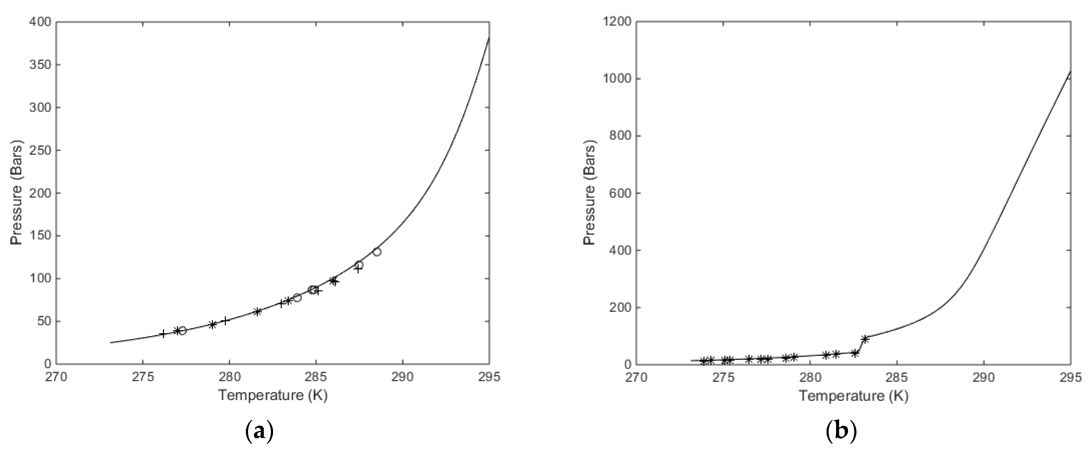
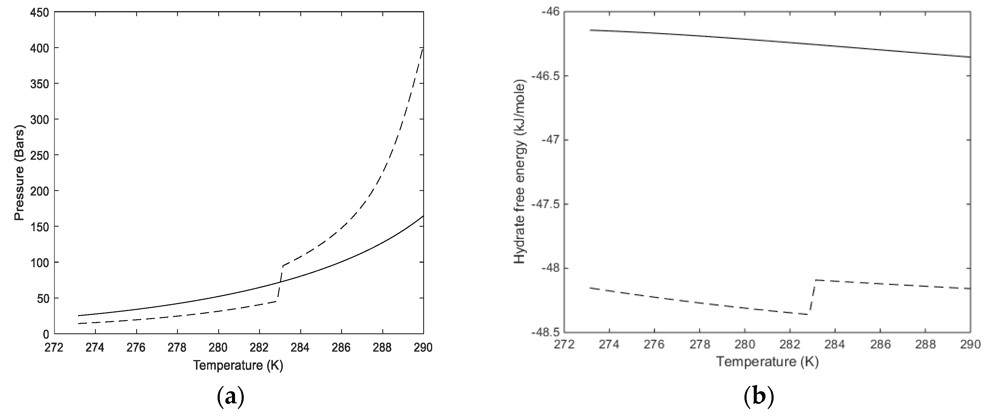
For the heterogeneous case we therefore first calculate the equilibrium curve. For pure CH
4 or pure CO
2, and a defined temperature, the chemical potential for the guest is given by Equation (9) for a variable pressure. This chemical potential enters Equation (4) along with the free energy of inclusion, which is a function of temperature only for small and large cavities. Equations (2) and (3) are solved for the same chemical potential of water in liquid state and hydrate given the equilibrium pressure. For completeness the free energies of inclusion are given in
Table 3 below. Calculated equilibrium curves for CH
4 and CO
2 are compared to experimental data in
Figure 2. It is important to keep in mind that the parameters for free energies of inclusion have been calculated from MD simulations with the procedures described in Kvamme and Tanaka [
12] for temperatures up to 280 K for CH
4. As such, all calculated results are predictions, and results for temperatures above 280 K are all extrapolations. For CO
2, on the other hand, a system of nine unit cells of hydrate structure I was surrounded on all sides with a 3 nm thick layer of CO
2 molecules. The system was run at 273.16 K and 283 K using SRK calculated densities in order to keep consistency with other calculations in this work that utilize the SRK equation of state. The system was then also run for 284 K and 290 K, which are both in the dense CO
2 region. The essential difference between the low temperature results and the high temperature results are the impact of the surrounding CO
2 molecules on the water lattice vibrations. The hydrate water structure is dominated by the 75% large cavities and the small cavity does not even benefit much from any stabilization of CO
2 due to the size and shape of the molecule. For the small cavities in structure I there is not statistical justification to distinguish between the effect of surround gas or liquid CO
2.
The models for extending thermodynamic properties of water and fluid phases are discussed in detail elsewhere [
19,
20,
21] and will not be repeated here due to space limitations.
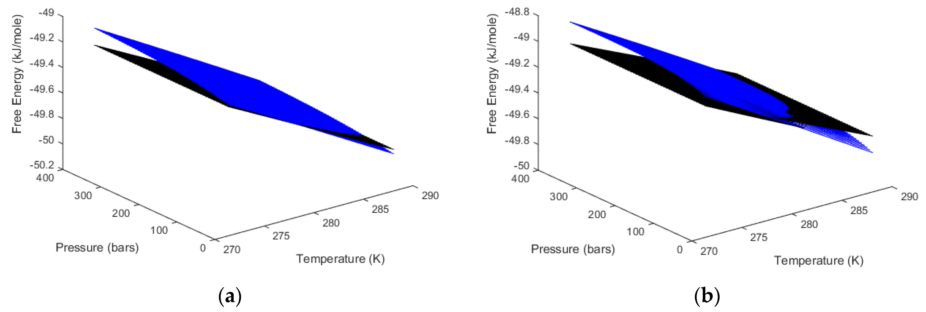
Two aspects regarding
Figure 2a,b are worth mentioning. The equilibrium curve for CO
2 in
Figure 2b does not have a discontinuity but there is a rapid change in density related to a phase transition. This leads to a rapid decrease in fugacity coefficients and a corresponding higher pressure needed to reach hydrate equilibrium. Some researchers actually presents
Figure 2b as a continuous smooth curve without any rapid change. A second aspect is illustrated in
Figure 2a. As can be seen, the equilibrium pressures for CO
2 hydrate are higher than the equilibrium pressures for CH
4 after the CO
2 density increase. This is often wrongly interpreted as a higher stability for the CH
4 hydrate above the temperature for the CO
2 phase transition. Pressure and temperature are independent thermodynamic variables. Free energies are the corresponding thermodynamic responses for the level of thermodynamic stability. In
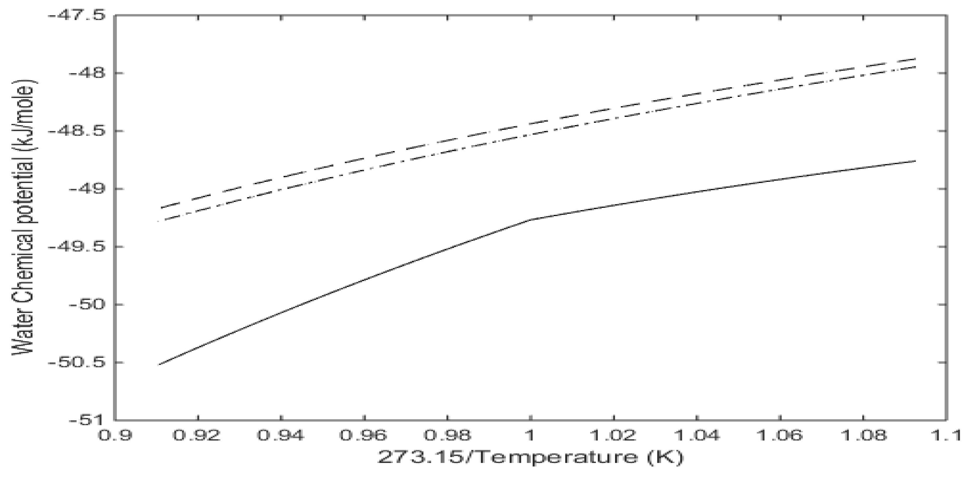
Figure 2b we plot free energies of CH
4 and CO
2 hydrate as function of temperature along the equilibrium pressures for the two types of hydrates.
Along the curves in
Figure 2 the free energy changes in Equation (1) are trivially zero. Outside equilibrium all properties of fluids are continuous and can be calculated for any pressure and temperature. The necessary pressure correction for water chemical potential in Equation (2) is available from the molar volume of liquid water, which is almost constant and independent of temperature and pressure, time pressure minus equilibrium pressure for the actual temperature. Hydrate water chemical potential, on the other hand, is based on an equilibrium theory. The derivation [
12] from the grand canonical ensemble in statistical mechanics leads to a Langmuir type of adsorption theory as expressed by Equation (3). For:
we choose
T to be equal to an equilibrium temperature, for which equilibrium pressure and compositions are calculated according to the equation and discussion above. The correction for pressure change is related to the partial molar volumes of water and hydrate formers in hydrate. Water partial molar volume is given by the structure of the hydrate while the occupation volume of the guest molecules can be calculated from Monte Carlo simulations according to the procedures described by Kvamme and Lund [
26] and Kvamme and Førridahl [
27]. The calculated volumes are 164.2 Å
3/molecule and 89.2 Å
3/molecule for CH
4 in large and small cavities, respectively. Corresponding values for CO
2 are 135.6 Å
3/molecule and 76.9 Å
3/molecule for large and small cavities, respectively. The value for CO
2 in small cavities is not practically interesting since the filling fractions of CO
2 in small cavities is practically zero.
Classical nucleation theory (CNT) for a spherical hydrate particle can be written as:
where
J0 is the mass transport flux supplying the hydrate growth. The phase transition in Equation (1) it will be the supply of CH
4 or CO
2 across an interface of gradually more structured water towards the hydrate core, as discussed in Kvamme et al. [
19,
20,
21]. The units of
J0 will be moles/m
2s for heterogeneous hydrate formation on the growing surface area of the hydrate crystal.
β is the inverse of the gas constant times temperature and Δ
GTotal is the molar free energy change of the phase transition. This molar free energy consists of two contributions (Equation (1) with Equation (10)) to correct for hydrate properties outside of equilibrium which are the free energy benefit of the phase transition and the second contribution is the penalty related to the work of pushing aside old phases. Even for a hydrate forming on the gas/water interface any hydrate core below critical size will be covered by water also on the side facing the gas due to capillary forces. Molar densities of liquid water and hydrate are reasonably close. It is therefore a fair approximation to multiply the molar free energy of the phase transition with molar density of hydrate times the volume of hydrate core. The penalty of the push work is the interface free energy times the surface area of the hydrate crystal. The total free energy change in extensive formulation (underlines indicate Joule units):
The simplest possible geometry of a crystal is a sphere and for a core radius
R the result is:
where
is the molar density of the hydrate and
is the interface free energy between the hydrate and the surrounding phase. There is no reliable value for interface free energy between hydrate and liquid water since the measurement of such a property is extremely difficult. We have not found any value in the open literature. Interface free energy between liquid water and ice is available [
28] and the reported value is 29.1 mJ/m
2. We have used this value as an approximation for interface free energy between liquid water and hydrate in the last term of Equation (13).
Differentiation of (13) with respect to
R gives the solution for maximum free energy radius (the critical core size):
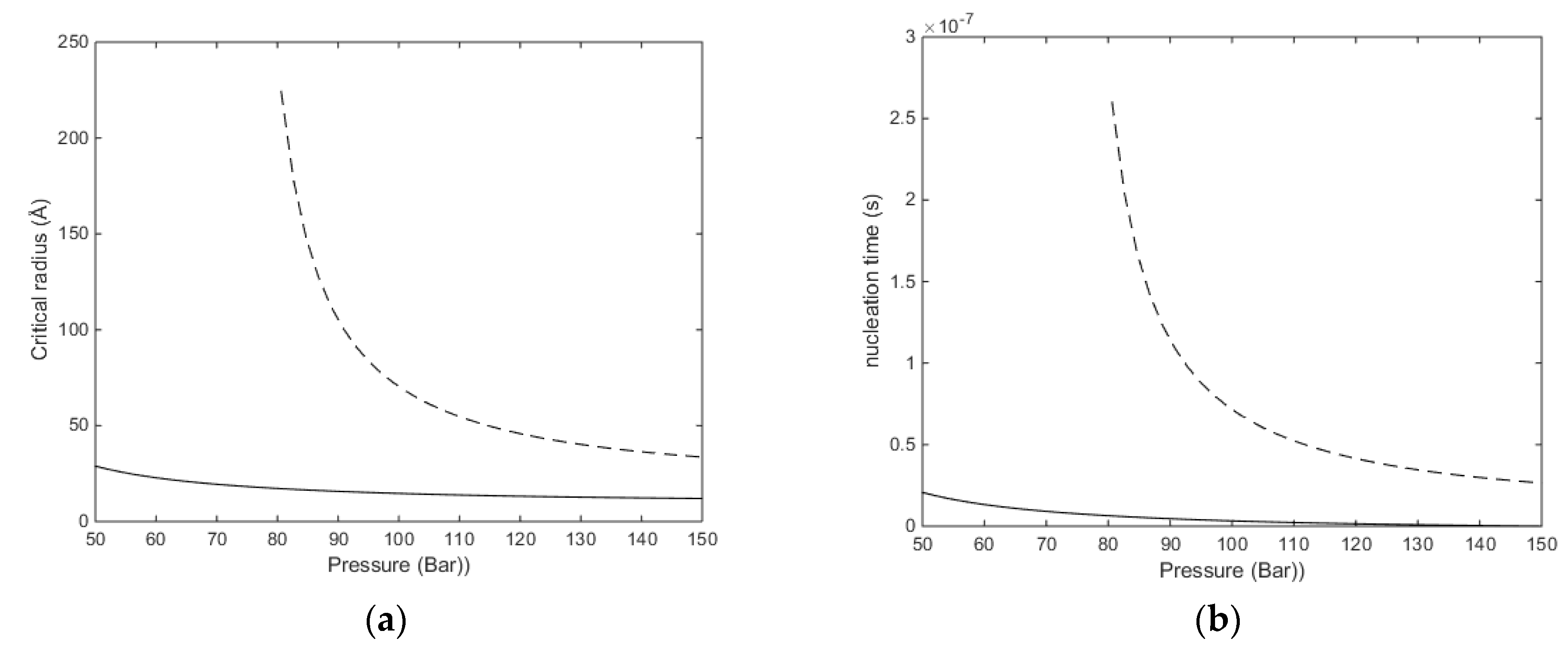
Superscript * denotes critical nuclei radius. Calculated critical radii for CH
4 hydrate at two different temperatures are given in
Figure 3a. The associated nucleation times are based on integration of Fick’s law:
The concentration profiles for CH
4 as a function of distance from the liquid side of the interface (
z = 0 Å) to the hydrate side of the interface (
z = 12 Å) is available from Kvamme [
19,
20] and Kvamme et al. [
21]. The diffusivity coefficient profile for CH
4 is assumed to be the same as for CO
2 since the diffusion of CH
4 and CO
2 through the liquid/water interface is dominated by the gradually increased structure of water towards the hydrate side of the interface. The profile is given by Figure 8a in Kvamme [
19] and fitted to Equation (16) with the parameters in
Table 4 below.
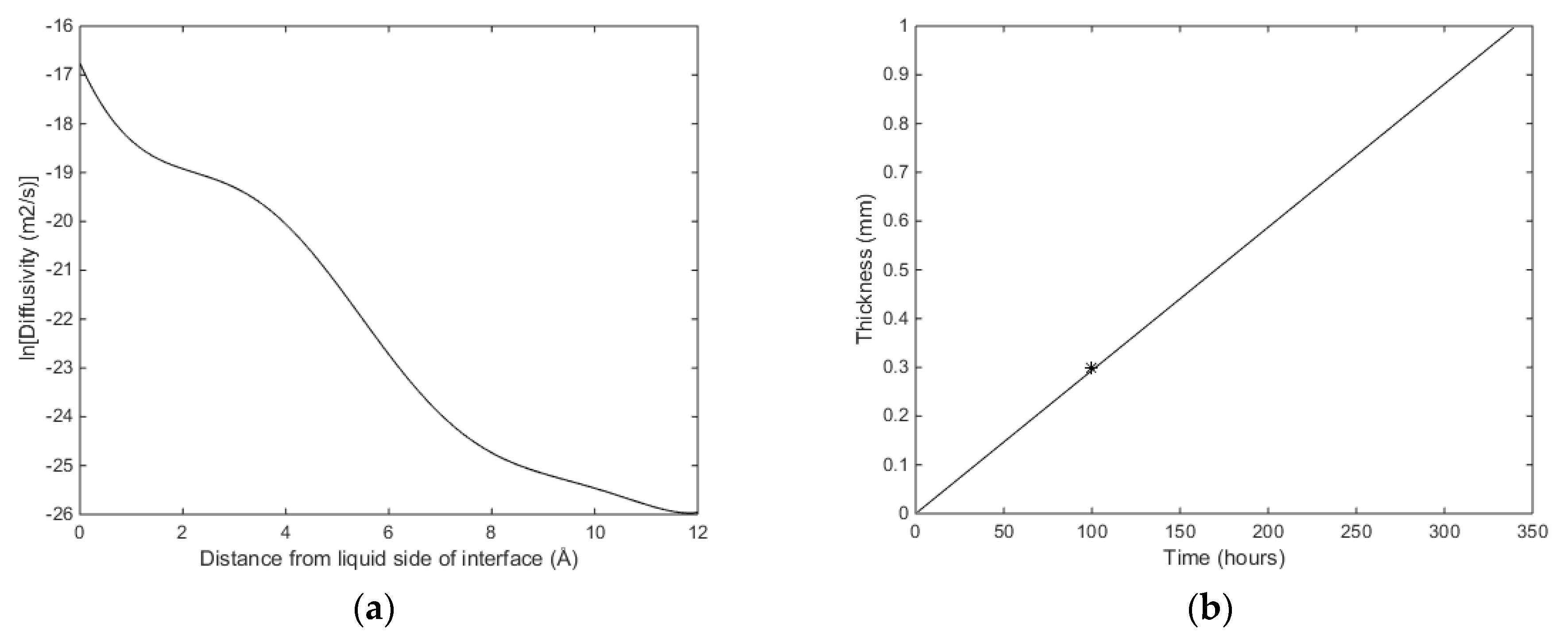
Using
Dliquid,j equal to 1.0·10
−08 m
2/s and integrating Equation (15) to critical size. That is, for every supply of hydrate-former needed to grow a hydrate core, the transport has to cross the interface thickness at the mass transport penalty given by Equation (16). The number of transported molecules is then recalculated to provide a corresponding radius added to the core size. This latter recalculation involves the calculated filling fraction and the corresponding volume of hydrate water. With reference to the equilibrium curve in
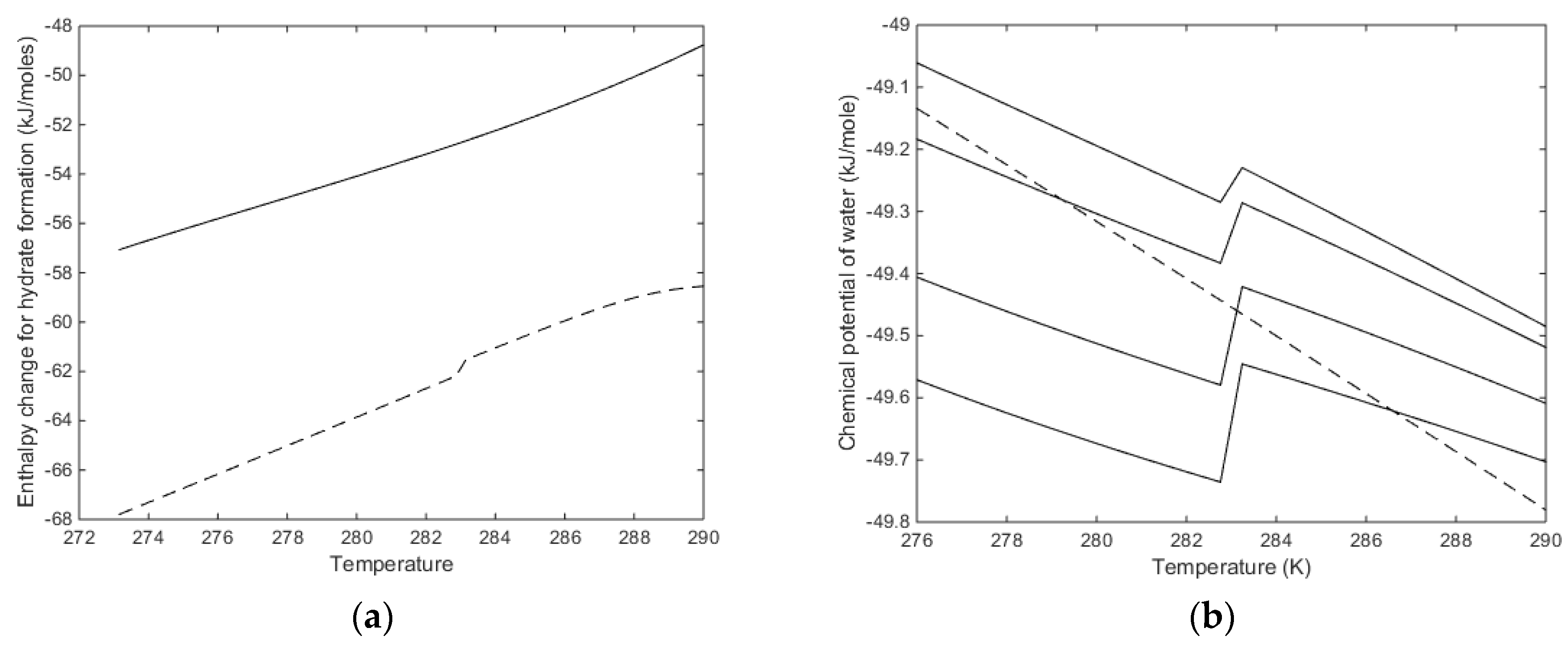
Figure 2a note that the equilibrium pressure for 283.16 K is around 80 bars and that is the reason for the exponential increase in critical size when the pressure approaches 80 bar. As expected, there is a substantial increase in nucleation time between these two temperatures. At 273.16 K and 150 bar the calculated critical radius is 12.0 Å and nucleation time is essentially instantaneous (less than one ns). Calculated critical radius at 283.16 K and 150 bars is 33.6 Å, and nucleation time is 26.5 ns.
For transport of CH
4 through the hydrate, in order to continue the growth of the film, it is now assumed that the diffusivity coefficient, and associated diffusion rate at the hydrate side of the interface, is equal to a stationary transport through the hydrate. This rate is expected to be slightly higher than regular diffusion through a block of hydrate without dynamics of couplings to heat transport and dynamic situations of partial local dissociation and reformation. See Kvamme et al. [
21] for a brief summary of reported diffusivities of hydrate-formers through hydrate. In summary the diffusivities range from 10
−15 m
2/s to 10
−17 m
2/s. Quite a number of the studies are based on Monte Carlo studies of “cavity jumping” and rarely reflect any mechanism for how guest molecules are actually able to move around in the hydrate structure. Based on our MD studies [
12] the mechanism seems more like a temporary destabilization of water hydrogen bonding structures between filled cavities and empty neighbor cavities. Nevertheless, more detailed studies are needed to verify these observations in a scientifically satisfactory manner. For our purpose in the context of this work we then might expect diffusivity coefficients which are higher than the range indicated above due to the couplings with heat transport dynamics rapid local dissociation/refreezing effects. The heat transport dynamics is implicitly coupled through the relationship:
which then connects Equations (12), (13) and (1) for any hydrate core since the number of moles in the actual radius of the core is simply the volume of the core times the molar density of the hydrate core. In the simple calculations below we disregard effects of heat transport dynamics. Based on our earlier calculations [
15,
16,
17,
18], and also in accordance with other sources in the literature, the heat transport rate through liquid water is 2–3 times faster than the corresponding mass transport rate. This ratio will be orders of magnitude higher for transport through hydrate. In accordance with this we expect that the mass transport rate is only affected by heat transport due to fast local phase transitions. Within the focus of this work we simply examine a couple of values for
Dliq in (16) and plot the time needed to reach 1 mm hydrate film thickness. In
Figure 4 we plot results for
Dliq = 5·10
−08 m
2/s in Equation (16) and the condition of temperature and pressure equal to that used in a magnetic resonance imaging experiment conducted at the ConocoPhillips research laboratory in Bartlesville (OK, USA). The experiment was conducted at a temperature of 276.25 K and 83 bars with initial equal volumes of liquid water and CH
4. See Kvamme et al. [
29] for more details on the experiment. The container was made of plastic and as such was methane-wetting.
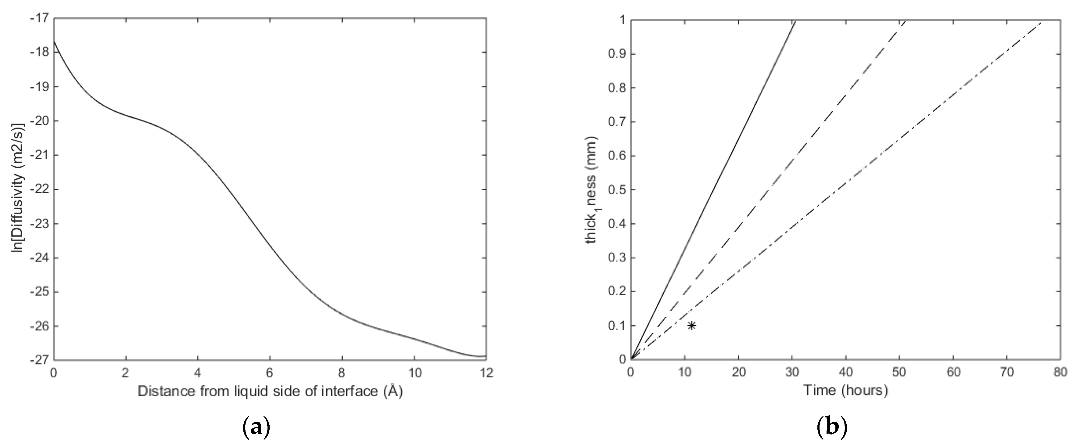
Nucleation studies for CO
2 have been published in a recent paper [
19] and in order to save space we limit ourselves to estimates of growth as illustrated in
Figure 5.
Based on the methods of Kvamme and Tanaka [
12] it is easy to see that water molecules between a filled cavity and a neighboring empty cavity have higher librational movements and hydrogen bonding structures can temporarily break and let guest molecules move to the empty cavity. For CH
4 this can happen for all cavities while for the larger CO
2 only large cavity neighbors can participate in such transports. As such it is reasonable that the diffusivity coefficient for CO
2, through hydrate, is lower than the corresponding values for CH
4. And just as macroscopic heat transport is orders of magnitude faster than mass transport so is the local molecular heat transport involved in breaking and reforming hydrogen water hydrogen bonds during migration of a guest molecule between cavities.
The mechanical strength of hydrate films in a pore depends on the cross section area, thickness and strength of connection to the mineral surfaces. As discussed in several papers, for instance [
32,
33] and papers referenced therein, hydrate can never touch the surface of minerals. From a thermodynamic point of view this can easily be verified in calculated and experimental structures of water. The density of the first adsorbed water layer on minerals such as calcite, hematite, and kaolinite is on the order of three times the density of liquid water. The associated chemical potential is very low and far lower than is ever possible for water in hydrate. Even the average chemical potential of adsorbed water as calculated over the first five layers of water adsorbed on Hematite may be as low as 3.4 kJ/mole lower than liquid water [
32]. The reason is the strong Coulombic interactions between water partial charges and charges on atoms in the mineral surfaces. For the same reason it is also easy to see that the regular distribution of partial charges on water hydrogens and oxygens in a hydrate crystal can never favorably match the distribution of positive and negative charges on the mineral surfaces.
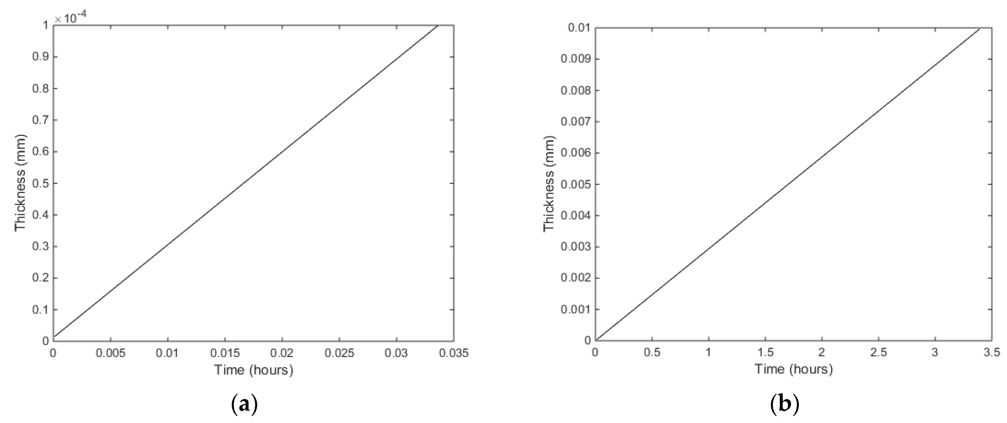
What we have presented above provides a tool for analyzing how rapidly the hydrate film will grow, and for specific porosity and minerals, when and at what frequency we need to shock the system in order to break these hydrate films during the formation of hydrate in a specific sediment model (or real sediment from coring) in a laboratory set-up. For this purpose we need a higher resolution time scale of the growth, and in
Figure 6 we plot the times needed to reach 100 nm and 10 micron (10,000 nm).
As discussed above it is a straightforward mechanical calculation to determine the magnitude of a mechanical pulse. If 100 nm is an acceptable thickness then the frequency of a mechanical shock pulse needs to be on the average 2 min. Depending on the laboratory set-up this pulse can be generated by sound, mechanical shaking of the sediments section etc. The important thing is that the sediments section is kept in place relative to circulation of fluids and that the mechanical pulse that is used to break the hydrate films is moderate according to the forces needed to break the hydrate films. The necessary force needed is sensitive to many factor like for instance pore size, geochemical issues (mineral types and salinity) as well as temperature and pressure. Calculations of necessary forces to break the hydrate films using mechanical pulses are therefore too case specific to discuss in a more general paper like this.
In the Ignik Sikumi test on hydrate production [
8,
9,
11] large amounts of N
2 were added and the thermodynamic driving force for creating a new CO
2 hydrate was practically lost [
9]. Instead of mechanically, breaking the hydrate films with efficient surfactants can keep the water/CO
2 interface free of blocking hydrate and permit for more continuous hydrate formation from the injected CO
2. Even methanol has surfactant properties but is too solvable in water to be interesting. And methanol is of course poisonous and not desirable to use. But some general insight can be found from a recent study [
21].


 ,
, 


