Adaptive Sliding Mode Trajectory Tracking Control for WMR Considering Skidding and Slipping via Extended State Observer

Abstract

When the wheeled mobile robot (WMR) is required to perform specific tasks in complex environment, i.e., on the forestry, wet, icy ground or on the sharp corner, wheel skidding and slipping inevitably occur during trajectory tracking. To improve the trajectory tracking performance of WMR under unknown skidding and slipping condition, an adaptive sliding mode controller (ASMC) design approach based on the extended state observer (ESO) is presented. The skidding and slipping is regarded as external disturbance. In this paper, the ESO is introduced to estimate the lumped disturbance containing the unknown skidding and slipping, parameter variation, parameter uncertainties, etc. By designing a sliding surface based on the disturbance estimation, an adaptive sliding mode tracking control strategy is developed to attenuate the lumped disturbance. Simulation results show that higher precision tracking and better disturbance rejection of ESO-ASMC is realized for linear and circular trajectory than the ASMC scheme. Besides, experimental results indicate the ESO-ASMC scheme is feasible and effective. Therefore, ESO-ASMC scheme can enhance the energy efficiency for the differentially driven WMR under unknown skidding and slipping condition.

1. Introduction

With the increasingly widespread application of robotics, wheeled mobile robot (WMR) is required to perform many tasks, i.e., rescue operation [1], transportation products [2], social interaction [3], planetary exploration [4] and so on. High-performance control strategy is the prerequisites to implement the different practical tasks efficiently. Therefore, the motion control problem has become the hotspot in the robotics field.

Due to the WMR is a typical nonholonomic system, most present researches on the tracking control schemes were base on assuming that the wheel rolling without considering slipping and skidding. A combined kinematic/torque controller was presented with the adaptive backstepping in [5], a finite-time tracking controller with output feedback was developed in [6], a data-based path tracking control algorithm was realized in [7,8], sliding-mode based algorithms [9,10,11] were presented to allow two different types of WMRs to track the reference path. [12,13,14,15] presented several other effective algorithms, such as the neural networks method [12], robust control scheme [13,14], and backstepping approach for path tracking control in [15]. Unfortunately, the controller in [5,6,7,8,9,10,11,12,13,14,15] had achieved certain performance on trajectory tracking based on nonslipping and nonskidding assumptions.

However, the WMRs do not always satisfy the nonslipping and nonskidding conditions when the WMRs are applied in some unknown and complex environment, i.e., on the forestry, wet or icy roads, on the sharp corner. As a result, wheel skidding and slipping may happen easily during the movement. Therefore, to tackle the tracking control problem for WMR considering wheel skidding and slipping affect, it is very necessary to design the control scheme for WMRs. Many approaches have been applied by the various researchers for WMR. GPS-based tracking strategy based on kinematics model was proposed for one car-like WMR considering skidding-slipping effect [16,17,18]. A robust tracking and regulation controller was developed using the kinematic model [19]. In terms of kinematics, Ramon et al. proposed an adaptive control approach using a linear matrix inequalities with slipping [20]. In [21], an adaptive tracking approach was presented, where the sliding model based observer was designed to online estimate the sliding parameter. The path tracking problem using kinematics model under consideration of the wheel skidding-slipping phenomena had achieved certain results. However, due to the nonlinearity and uncertainty exists in WMR, consequently another framework in dynamics were proposed to address the tracking problem for WMRs under the wheel skidding and slipping condition.

In general, the existing control schemes can be divided into two main groups, the one was the adaptive control scheme and the other was the robust tracking control scheme. With the unknown longitudinal slipping, an improved adaptive control strategy was proposed for the trajectory tracking, where the neural network online weight tuning algorithm was designed to ensure the tracking error [22]. A neural network tracking approach was developed via reinforcement learning to track the desired trajectory. The WMR was regarded as nonlinear discrete-time dynamic system in the motion control when the skidding and slipping phenomena existed [23]. For another robust tracking controller in presence of skidding and slipping, a desired virtual velocity controller based on disturbance observer (DOB) was developed in [24], a generalized extended state observer [25] and fuzzy disturbance observer [26] were developed. In the controller, the skidding and slipping was regarded as disturbance and thus the dynamics equation was modified. An improved disturbance attenuation controller was designed in [27] to solve the reference trajectory tracking when the lateral and longitudinal slippage existed. Specifically, the tracking differentiator and nonlinear state error feedback was introduced into the controller, thus the disturbance attenuation can be achieved.

As one practical solution for disturbance attenuation, DOB is developed to estimate the disturbance from system state or output measurement and introduce the estimation result to eliminate the disturbance effect in the system. [28,29] As a fundamental part of active disturbance attenuation, extended state observer (ESO) was first proposed by Han [30] to reject the lumped disturbance containing both uncertainty and the external disturbance [27,31,32]. Besides, the main characteristics of the sliding mode controller possesses the maim characteristics, i.e., overcoming the system uncertainty and strongly robust on parameter uncertainty and disturbance [33]. Especially for nonlinear system, adaptive sliding mode control (ASMC) strategy is used to weaken the chattering phenomenon [34].

Therefore, to track the desired trajectory of WMR with consideration of unknown skidding and slipping effect, an adaptive sliding mode tracking approach via an extended state observer is presented. The proposed controller combines the advantage of sliding mode control and extended state observer, thus can effectively compensate the disturbance influence. For the existing unknown skidding and slipping, it is regarded as disturbance. The ESO is introduced to estimate the lumped disturbance, an adaptive sliding surface based on the disturbance estimation is developed to counteract the lumped disturbance.

The remainder of this paper is organized as follows. Section 2 describes in detail the problem formulation and preliminaries of the WMR system. The ESO-ASMC tracking controller is designed in Section 3. Simulation results are given to illustrate the tracking performance of the ESO-ASMC controller in Section 4. Experimental platform is built up and practical tests are carried out in Section 5, to validate the practicality of the ESO-ASMC control approach. Finally, Section 6 gives the conclusion.

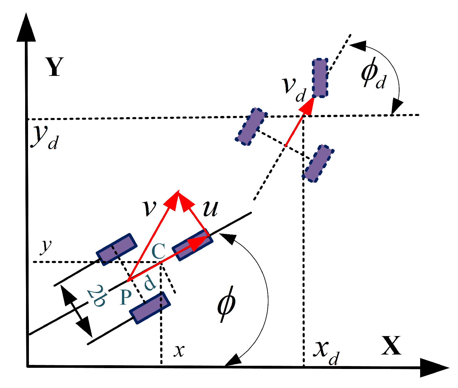
2. Problem Formulation and Preliminaries

A typical example of a differentially driven mobile robot used for tracking research is studied in this section. As depicted in Figure 1, the self-developed WMR composes of two driving wheels, a front wheel used for supporting the robotic platform and without guiding function. The motion of the WMR is actuated by two direct drive motors of the driving wheel. Although the two direct drive motors are mounted independently, each drive motor has almost the same characteristics, i.e., position, velocity, force response, friction model and other nonlinear phenomenon.

The dynamic equation of the differentially driven WMR in the Lagrange form [21,22,23,24] is:

$$M\left(q\right)\ddot{q}+V\left(q,\dot{q}\right)\dot{q}+G\left(q\right)+{\tau }_d=T\left(q\right)\tau -A^T\left(q\right)\lambda ,$$

(1)

where $q={\left[x,y,\varphi ,{\psi }_r,{\psi }_l\right]}^T\in {\Re }^{\mathrm{n}}$ is the generalized coordinates, $x,y$ and $\varphi$ describe the position and forward direction angle. ${\psi }_r$ and ${\psi }_l$ present the angular position of the right and left driving wheel, $M\left(q\right)\in {\Re }^{\mathrm{n}\times n}$ is a symmetric, positive definite inertia matrix, $V\left(q,\dot{q}\right)\in {\Re }^{\mathrm{n}\times n}$ is the centripetal and Coriolis matrix, $G\left(q\right)\in {\Re }^{\mathrm{n}}$ is the gravitational vector, ${\tau }_d\in {\Re }^{5\times 1}$ denotes the bounded external disturbances, $T\left(q\right)\in {\Re }^{n\times r}$ is the input transformation matrix, $\tau$ is the input torque provided by the two direct drive motors, $A\left(q\right)\in {\Re }^{\mathrm{m}\times n}$ is the matrix associated with the constraints, and $\lambda \in {\Re }^{\mathrm{m}}$ is the vector of constraint force. As the WMR in the paper operates on the even ground, the gravitational vector $G\left(q\right)\in {\Re }^{\mathrm{n}}$ equals zero.

From Figure 1 we can see, the centroid C of WMR does not coincide with geometric center P. The nonholonomic constraints of WMR are expressed as:

$$\left\{\begin{array}{c}-\dot{x}sin\varphi +\dot{y}cos\varphi -d\dot{\varphi }=0\\ \dot{x}cos\varphi +\dot{y}sin\varphi +b\dot{\varphi }=r{\dot{\psi }}_r\\ \dot{x}cos\varphi +\dot{y}sin\varphi -b\dot{\varphi }=r{\dot{\psi }}_l\end{array},\right.$$

(2)

where $\dot{x}$ and $\dot{y}$ are the generalized velocity defined in the inertial coordinate system, ${\dot{\psi }}_r$ and $\dot{{\psi }_r}$ represent the angular velocity of the two driving wheels. d is the distance between the centroid and the geometric center of WMR platform, b is the half width of the WMR and r is the wheel radius. Equation (2) can be rewritten as:

$$A\left(q\right)\dot{q}=0,$$

(3)

where $A\left(q\right)=\left[\begin{array}{ccc}-sin\varphi & cos\varphi & \begin{array}{ccc}-d& 0& 0\end{array}\\ cos\varphi & sin\varphi & \begin{array}{ccc}b& -r& 0\end{array}\\ cos\varphi & sin\varphi & \begin{array}{ccc}-b& 0& -r\end{array}\end{array}\right]$ is the nonholonomic constraint matrix.

Based on Equation (3), a matrix $J\left(q\right)$ is defined to satisfy $A\left(q\right)J\left(q\right)=0$, where $J\left(q\right)=\left[\begin{array}{cc}cos\varphi & -dsin\varphi \\ \begin{array}{c}sin\varphi \\ 0\\ \frac{1}{r}\\ \frac{1}{r}\end{array}& \begin{array}{c}dcos\varphi \\ 1\\ \frac{b}{r}\\ -\frac{b}{r}\end{array}\end{array}\right]$.

With the expansion of WMR applications, the kinematic model does not always meet the skidding and nonslipping constraint in some special situation. The kinematic equation of the WMR considering unknown skidding-slipping effect is:

$$\left\{\begin{array}{c}-\dot{x}sin\varphi +\dot{y}cos\varphi -d\dot{\varphi }=u\\ \dot{x}cos\varphi +\dot{y}sin\varphi +b\dot{\varphi }=r\left({\dot{\psi }}_r-{\theta }_r\right)\\ \dot{x}cos\varphi +\dot{y}sin\varphi -b\dot{\varphi }=r\left({\dot{\psi }}_l-{\theta }_l\right)\end{array},\right.$$

(4)

where u denotes the lateral skidding velocity, ${\dot{\theta }}_r$ and ${\dot{\theta }}_l$ present the perturbed angular velocity caused by wheel slipping. Equation (4) can be put into matrix form:

$$A\left(q\right)\dot{q}={\left[u,-r{\theta }_r,-r{\theta }_l\right]}^T.$$

(5)

With regard to the skidding and slipping in the movement, the kinematic equation of the WMR is:

$$\dot{q}=J\left(q\right)\left(\zeta -\delta \right)+N\left(q\right)p_0,$$

(6)

where $\zeta ={\left[v,w\right]}^T$, $v=r\left({\dot{\psi }}_r+{\dot{\psi }}_l\right)/2$ denotes the forward linear velocity, $w=r\left({\dot{\psi }}_r-{\dot{\psi }}_l\right)/2b$ is the angular velocity. $\delta ={\left[{\delta }_v,{\delta }_w\right]}^T$, ${\delta }_v=r\left({\theta }_r+{\theta }_l\right)/2$ denotes the longitudinal slipping velocity, ${\delta }_w=r\left({\theta }_r-{\theta }_l\right)/\left(2b\right)$ is the perturbed angular velocity. $N\left(q\right)p_0$ denotes the unmatched disturbance matrix due to the perturbed nonholonomic constraint, and:

$$N\left(q\right)=\left[\begin{array}{ccc}-sin\varphi & 0& 0\\ cos\varphi & 0& 0\\ \begin{array}{c}0\\ 0\\ 0\end{array}& \begin{array}{c}0\\ 1\\ 0\end{array}& \begin{array}{c}0\\ 0\\ 1\end{array}\end{array}\right],p_0={\left[u,{\theta }_r,{\theta }_l\right]}^T.$$

Assumption 1.

The perturbation δ, u, and also their first, second, third derivatives are bounded. In addition, perturbation δ, u and their derivatives are relatively small compared with the reference velocity [24].

The derivation of Equation (6) is

$$\ddot{q}=\dot{J}\left(q\right)\left(\zeta -\delta \right)+J\left(q\right)\left(\dot{\zeta }-\dot{\delta }\right)+\dot{N}\left(q\right)p_0+N\left(q\right){\dot{p}}_0$$

(7)

Substituting Equation (7) into Equation (1), the dynamic formula of the WMR in presence of skidding and slipping is:

$$S_1\left(q\right)\left(\dot{\zeta }-\dot{\delta }\right)+U_1\left(q,\dot{q}\right)\left(\zeta -\delta \right)+P_1\left(q\right){\dot{p}}_0+P_2\left(q\right)p_0+P_3\left(q\right)+{\tau }_d=\tau ,$$

(8)

where:

$$\begin{array}{cc}\hfill S_1\left(q\right)& ={\left(J^T\left(q\right)T\left(q\right)\right)}^{-1}{J}^T\left(q\right)M\left(q\right)J\left(q\right),\hfill \\ \hfill U_1\left(q,\dot{q}\right)& ={\left(J^T\left(q\right)T\left(q\right)\right)}^{-1}{J}^T\left(q\right)\left[M\left(q\right)\dot{J}\left(q\right)+V\left(q,\dot{q}\right)J\left(q\right)\right],\hfill \\ \hfill P_1\left(q\right)& ={\left(J^T\left(q\right)T\left(q\right)\right)}^{-1}{J}^T\left(q\right)M\left(q\right)\mathrm{N}\left(q\right),\hfill \\ \hfill P_2\left(q\right)& ={\left(J^T\left(q\right)T\left(q\right)\right)}^{-1}{J}^T\left(q\right)\left[M\left(q\right)\dot{N}\left(q\right)+V\left(q,\dot{q}\right)N\left(q\right)\right],\hfill \\ \hfill P_3\left(q\right)& ={\left(J^T\left(q\right)T\left(q\right)\right)}^{-1}{J}^T\left(q\right)G\left(q\right).\hfill \end{array}$$

Property 1.

Reference [26]: $S_1\left(q\right)$ is symmetric and positive-definite, and $\left(\dot{\overline{M}}\left(q\right)-2\overline{V}\left(q\right)\right)$ is skew-symmetric, where $S_1\left(q\right)={\left(\overline{T}\left(q\right)\right)}^{-1}\overline{M}\left(q\right)$, $\overline{T}\left(q\right)=J^T\left(q\right)T\left(q\right)$, $\overline{M}\left(q\right)=J^T\left(q\right)M\left(q\right)J\left(q\right)$, $\overline{V}\left(q,\dot{q}\right)=J^T\left(q\right)\left[M\left(q\right)\dot{J}\left(q\right)+V\left(q,\dot{q}\right)J\left(q\right)\right]$.

As the WMR execute work on the level surface, we obtain gravity vector $G\left(q\right)$ equals zero and $P_3\left(q\right)$ equals zero. Considering Equation (8), we have:

$$\dot{\zeta }=U_2\left(q,\dot{q}\right)\zeta +S_2\left(q\right)\tau -U_2\left(q,\dot{q}\right)\delta +\dot{\delta }-S_2\left(q\right)\left[P_1\left(q\right){\dot{p}}_0+P_2\left(q\right)p_0\right]-S_2\left(q\right)P_3\left(q\right)-S_2\left(q\right){\tau }_d,$$

(9)

where $S_2\left(q\right)=S_1^{-1}\left(q\right),U_2\left(q,\dot{q}\right)=-S_1^{-1}\left(q\right)U_1\left(q,\dot{q}\right)$.

In addition, parameter uncertainty and parameter variation is considered due to the $S_2\left(q\right),U_2\left(q,\dot{q}\right)$ is determined by q. Equation (9) can be simplified as:

$$\dot{\zeta }=f\left(\zeta \right)+S_2\left(q\right)\tau +D,$$

(10)

where $f\left(\zeta \right)=U_2\left(q,\dot{q}\right)\zeta$, $D=-U_2\left(q,\dot{q}\right)\delta +\dot{\delta }-S_2\left(q\right)\left[P_1\left(q\right){\dot{p}}_0+P_2\left(q\right)p_0\right]-S_2\left(q\right){\tau }_d+\Delta U_2\left(q,\dot{q}\right)\zeta +\Delta S_2\left(q\right)\tau$, $\Delta U_2\left(q,\dot{q}\right),\Delta S_2\left(q\right)$ are parameter uncertainty and parameter variation caused by the driving wheel’s skidding and slipping.

Remark 1.

D denotes the compound disturbance, i.e., skidding and slipping of the driving wheel, input disturbance, parameter variation, and parameter uncertainty such as mass, moment of inertia, etc. And according to Assumption 1, D is bounded.

3. Tracking Problem for a Nonholonomic WMR

Before discussing the path tracking approach, in the inertial coordinate system the pose is defined as $q\left(t\right)={\left[x,y,\varphi \right]}^T$ and reference pose as $q_d\left(t\right)={\left[x_d,y_d,{\varphi }_d\right]}^T$ for the WMR.

Assumption 2.

At any time, v or w for the reference trajectory is nonzero simultaneously.

From the above analysis we can see, under the Assumption 2, the trajectory tracking control problem for WMR is to find the bounded control input $\tau =\left[\begin{array}{c}{\tau }_1\\ {\tau }_2\end{array}\right]$ to realize the tracking error $q_e={\left[\begin{array}{ccc}{x}_e& y_e& {\varphi }_e\end{array}\right]}^T$ bounded with $\underset{t\to \infty }{lim}∥q_e∥=0$ for the arbitrary initial error.

Specifically, the tracking error is:

$$q_e=\left[\begin{array}{c}{x}_e\\ y_e\\ {\varphi }_e\end{array}\right]=\left[\begin{array}{ccc}cos\varphi & sin\varphi & 0\\ -sin\varphi & cos\varphi & 0\\ 0& 0& 1\end{array}\right]\left[\begin{array}{c}{x}_d-x\\ y_d-y\\ {\varphi }_d-\varphi \end{array}\right].$$

(11)

The derivation of $q_e$ can be written as:

$${\dot{q}}_e=\left[\begin{array}{c}{v}_{d}cos{\varphi }_e-v+y_e\dot{\varphi }\\ v_{d}sin{\varphi }_e-x_e\dot{\varphi }\\ w_d-\dot{\varphi }\end{array}\right].$$

(12)

The auxiliary velocity is defined as [28]:

$${\zeta }_c=\left[\begin{array}{c}{v}_c\\ w_c\end{array}\right]=\left[\begin{array}{c}{v}_{d}cos{\varphi }_e+k_1{x}_e\\ w_d+v_d\left(k_2{y}_e+k_{3}sin{\varphi }_e\right)\end{array}\right],$$

(13)

where $k_1,k_2,k_3$ are the positive parameters to be designed.

The derivation of ${\zeta }_c$ is:

$${\dot{\zeta }}_c=\left[\begin{array}{c}{\dot{v}}_c\\ {\dot{w}}_c\end{array}\right]=\left[\begin{array}{c}{\dot{v}}_{d}cos{\varphi }_e\\ {\dot{w}}_d+k_2{\dot{v}}_d{y}_e\end{array}\right]+\left[\begin{array}{ccc}\begin{array}{c}{k}_1\\ 0\end{array}& \begin{array}{c}0\\ k_2{v}_d\end{array}& \begin{array}{c}-v_{d}sin{\varphi }_e\\ k_3{v}_{d}cos{\varphi }_e\end{array}\end{array}\right]{\dot{q}}_e.$$

(14)

Assuming the reference velocity is constant, we obtain:

$${\dot{\zeta }}_c=\left[\begin{array}{c}{\dot{v}}_c\\ {\dot{w}}_c\end{array}\right]=\left[\begin{array}{ccc}\begin{array}{c}{k}_1\\ 0\end{array}& \begin{array}{c}0\\ k_2{v}_d\end{array}& \begin{array}{c}-v_{d}sin{\varphi }_e\\ k_3{v}_{d}cos{\varphi }_e\end{array}\end{array}\right]{\dot{q}}_e.$$

(15)

The auxiliary velocity tracking error [24] is introduced using the backstepping approach:

$$e\left(t\right)={\zeta }_c-\zeta =\left[\begin{array}{c}{v}_c-v\\ w_c-w\end{array}\right].$$

(16)

Now, the control target is to design one torque input to satisfy $\underset{t\to \infty }{lim}e\left(t\right)=0$ and $\underset{t\to \infty }{lim}{q}_e\left(t\right)=0$.

The Lyapunov function candidate for ${\zeta }_c$ is defined as:

$$V_0=\frac{1}{2}\left(x_{\mathrm{e}}^2+y_{\mathrm{e}}^2\right)+\frac{1}{K_2}\left(1-cos{\varphi }_e\right).$$

(17)

The derivative of Equation (17) with respect to time yields:

$$\begin{array}{cc}\hfill {\dot{V}}_0=& {\dot{x}}_e{x}_e+{\dot{y}}_e{y}_e+\frac{1}{k_2}{\dot{\varphi }}_{e}sin{\varphi }_e\hfill \\ & =\left(v_{d}cos{\varphi }_e-v+y_e\dot{\varphi }\right)x_e+\left(v_{d}sin{\varphi }_e-x_e\dot{\varphi }\right)y_e+\frac{1}{k_2}\left(w_d-\dot{\varphi }\right)sin{\varphi }_e\hfill \\ & =\left(\left(w_d+v_d\left(k_2{y}_e+k_{3}sin{\varphi }_e\right)\right)y_e-\left(v_{d}cos{\varphi }_e+k_1{x}_e-{\psi }_v\right)+v_{d}cos{\varphi }_e\right)x_e\hfill \\ & +\left(v_{d}sin{\varphi }_e-x_e\left(w_d+v_d\left(k_2{y}_e+k_{3}sin{\varphi }_e\right)\right)\right)y_e+\frac{1}{k_2}\left(w_d-\left(w_d+v_d\left(k_2{y}_e+k_{3}sin{\varphi }_e\right)\right)\right)sin{\varphi }_e\hfill \\ & =w_d{x}_e{y}_e+v_d\left(k_2{y}_e+k_{3}sin{\varphi }_e\right)x_e{y}_e-k_1{x_e}^2+v_{d}sin{\varphi }_e{y}_e\hfill \\ & -x_e{w}_d{y}_e-x_e{v}_d\left(k_2{y}_e+k_{3}sin{\varphi }_e\right)y_e-\frac{1}{k_2}{v}_d\left(k_2{y}_e+k_{3}sin{\varphi }_e\right)sin{\varphi }_e\hfill \\ & =-k_1{x_e}^2-\frac{1}{k_2}{v}_d{k}_3{sin}^2{\varphi }_e\le 0\hfill \end{array}.$$

(18)

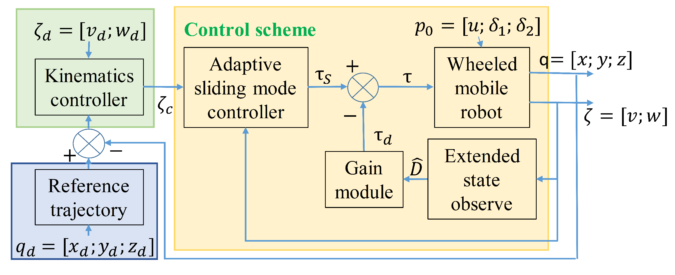
4. Controller Design and Stability Analysis

Considering the uncertainty such as modeling error, parameter perturbation and disturbance of WMR, the tracking controller is designed base on the kinematics and dynamics, to track the following trajectory under the condition of skidding and slipping.

4.1. Design of the Extended State Observer (ESO)

As the key step of the active disturbance rejection control, ESO regards the uncertainty as a new state and observes the state by output feedback. For the system in Equation (10), let $x_1=\zeta ,x_2=\dot{\zeta }$, the system can be extended as:

$$\left\{\begin{array}{c}{\dot{x}}_1=x_2\hfill \\ {\dot{x}}_2=x_3+f\left(x_1\right)+S_2\left(q\right)\tau \hfill \\ {\dot{x}}_3=h\hfill \end{array},\right.$$

(19)

where $x_3$ is the extended state representing the lumped disturbance term.

To estimate the disturbance D, the ESO is introduced and depicted as:

$$\left\{\begin{array}{c}{e}_1=z_1-y\hfill \\ {\dot{z}}_1=z_2-{\beta }_{01}{e}_{01}\hfill \\ {\dot{z}}_2=z_3-{\beta }_{02}fal\left(e_{01}\right)+S_2\left(q\right)\tau \hfill \\ {\dot{z}}_3=-{\beta }_{03}fal\left(e_{01}\right)\hfill \end{array},\right.$$

(20)

where $z_1$ denotes the estimation of $\zeta ,z_2$ denotes the estimation of $\dot{\zeta },z_3$ denotes the estimation of disturbances D. $e_{0i}=z_i-x_i$ is the estimation error, ${\beta }_{01},{\beta }_{02},{\beta }_{03}$ is the observer gain to be designed. $fal\left(•\right)$ is the nonlinear function defined as $fal\left(e_1,{\alpha }_i,\sigma \right)=\left\{\begin{array}{c}{∥e_1∥}^{{\alpha }_i}sign\left(e_1\right),∥e_1∥>\sigma \\ \frac{e_1}{{\sigma }^{1-{\alpha }_i}},∥e_1∥\le \sigma \end{array},i=1,2\right.$ where $\sigma$ is the length of the linear interval, $0<{\alpha }_i<1$.

Theorem 1.

For the given $\sigma >0$, if the ${\alpha }_1,{\alpha }_2,{\beta }_i,i=1,2,3$ are appropriately chosen, and satisfy the following condition:

$$\left\{\begin{array}{c}0<{\alpha }_2\le {\alpha }_1\le 1\hfill \\ 0<{\beta }_1<{\beta }_2<{\beta }_3\hfill \\ {\beta }_3<{\beta }_1{\beta }_2{\sigma }^{({\alpha }_l-{\alpha }_2)}\hfill \end{array}.\right.$$

(21)

The estimation error of ESO can exponentially converge to a small neighborhood of the origin.

The Proof of Theorem 1 can be seen in Appendix A.

4.2. Design of the Adaptive Sliding Mode Controller

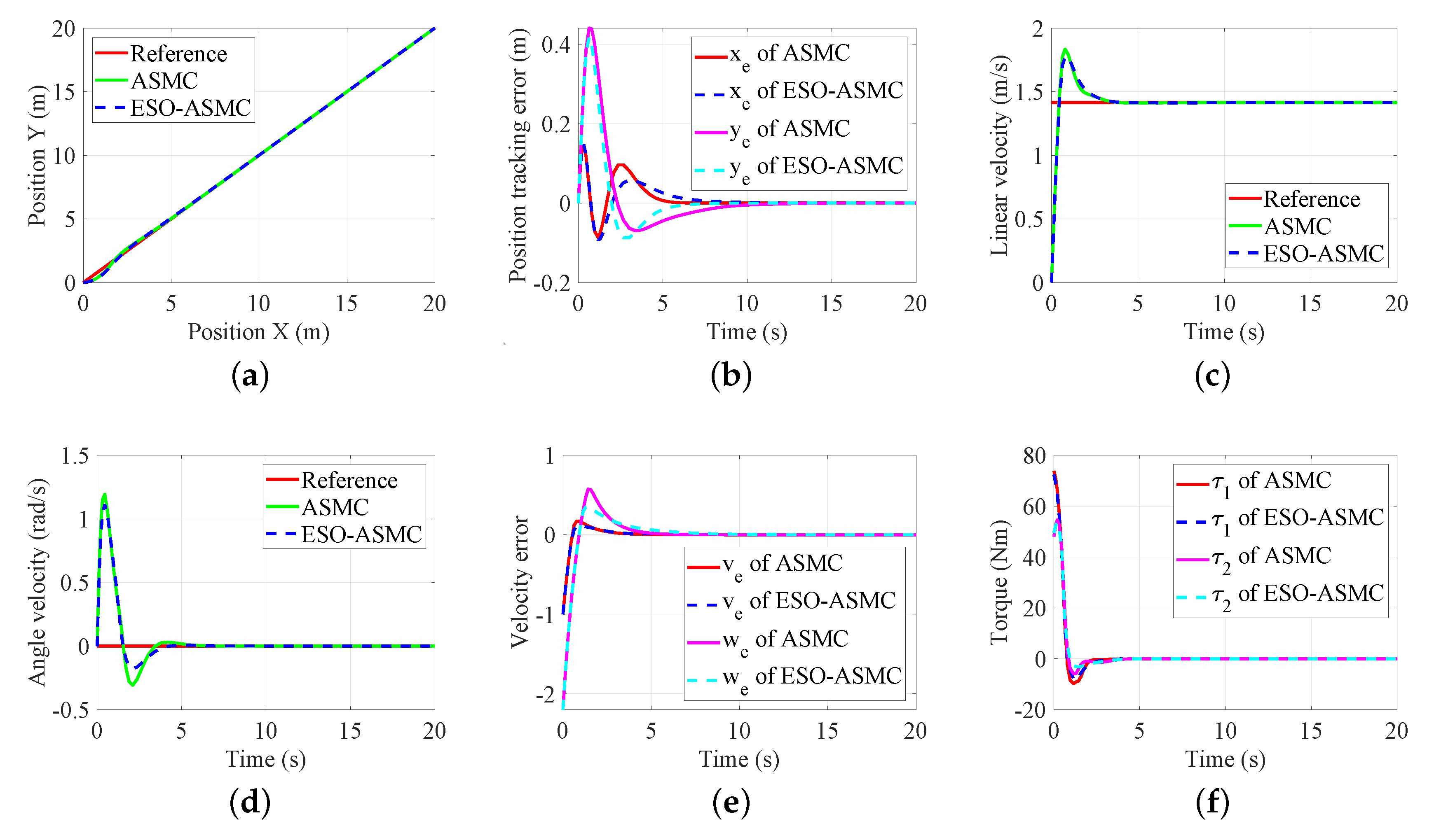
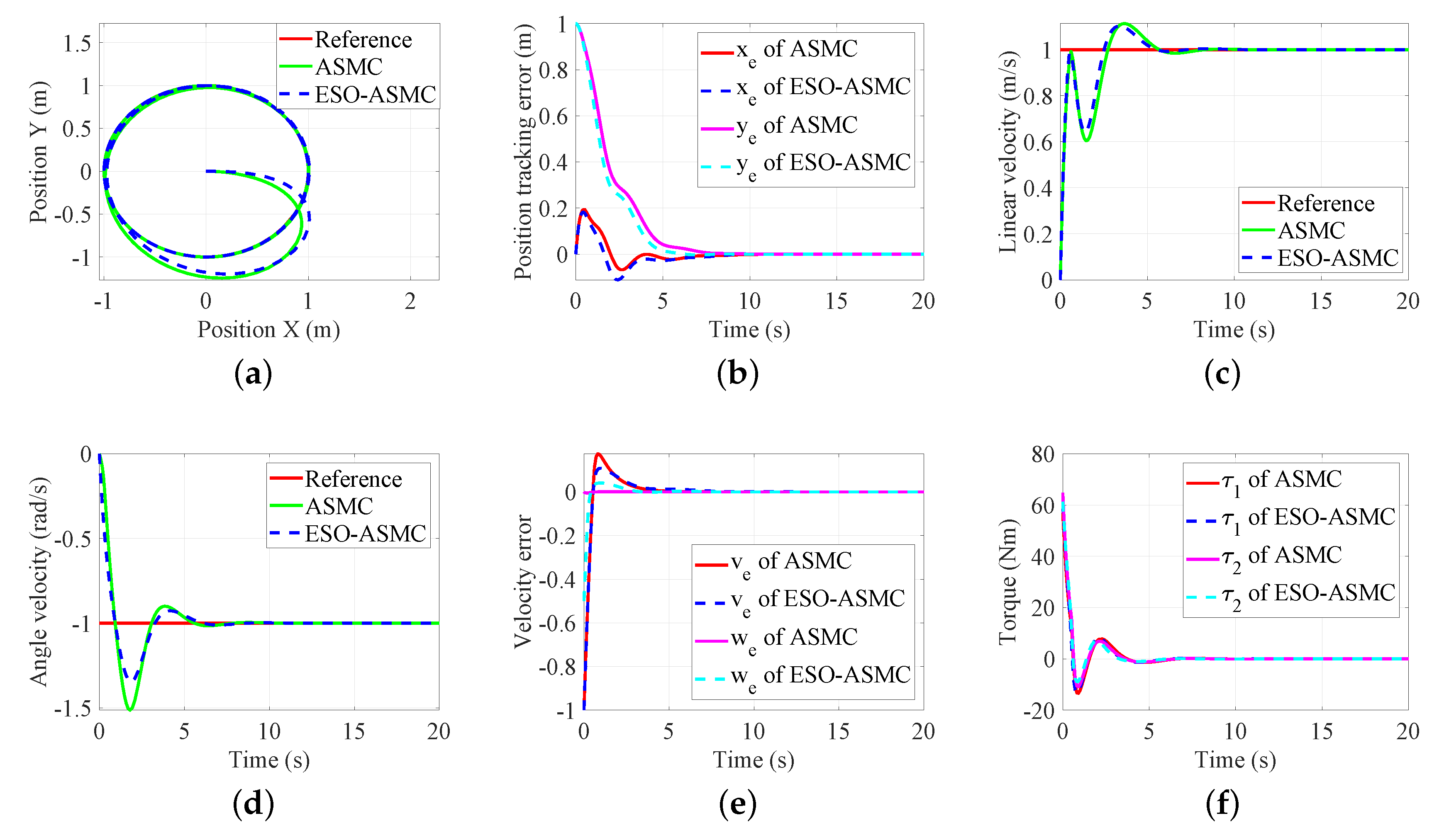
Due to the integral sliding model control is an efficient solution for counteracting the disturbance, in this subsection, to further improve the tracking control performance, based on the ESO in Equation (19), the integral sliding-mode control scheme for the WMR system is applied to compensate the un-observation disturbance. When ESO is adopted, Equation (10) can be given as

$$\begin{array}{cc}\hfill \dot{\zeta }=& f\left(\zeta \right)+S_2\left(q\right)\left({\tau }_S-{\tau }_D\right)+D\hfill \\ \hfill =& f\left(\zeta \right)+S_2\left(q\right){\tau }_S-\widehat{D}+D\hfill \\ \hfill =& f\left(\zeta \right)+S_2\left(q\right){\tau }_S+\tilde{D}\hfill \end{array}$$

(22)

It can be seen that the disturbance in Equation (10) is decreased. The Equation (22) can be expressed as

$$\dot{\zeta }=f\left(\zeta \right)+S_2\left(q\right){\tau }_S+\tilde{D}$$

(23)

The sliding surface is designed as

$$s\left(t\right)=e\left(t\right)+\Lambda \underset{0}{\overset{t}{\int }}e\left(\tau \right)d\tau$$

(24)

where $\Lambda =\left[\begin{array}{cc}{\lambda }_1& 0\\ 0& {\lambda }_2\end{array}\right]$ is a control parameter to be designed.

The derivation of s is

$$\begin{array}{cc}\hfill \dot{s}=& \dot{e}\left(t\right)+\Lambda e\left(t\right)={\dot{\zeta }}_c-\dot{\zeta }+\Lambda e\left(t\right)\hfill \\ \hfill =& {\dot{\zeta }}_c-\left[f\left(\zeta \right)+S_2\left(q\right){\tau }_S+\tilde{D}\right]+\Lambda e\left(t\right)\hfill \end{array}$$

(25)

The integral sliding-model controller based on nonlinear DOB is given as

$${\tau }_S={S_2}^{-1}\left(q\right)\left[{\dot{\zeta }}_c-f\left(\zeta \right)+\Lambda e\left(t\right)+\widehat{\mu }sign\left(s\right)\right]$$

(26)

where $\widehat{\mu }$ is the estimation of $\tilde{D}$ with estimation error $\tilde{\mu }=\mu -\widehat{\mu }$, $\mathrm{sign}\left(s\right)={\left[\begin{array}{cc}\mathrm{sign}\left(s_1\right)& \mathrm{sign}\left(s_2\right)\end{array}\right]}^T$. The adaptive control law is

$$\dot{\widehat{\mu }}=\eta \times \left|s\right|$$

(27)

where $\eta >0$ is the gain of adaptive control law.

Theorem 2.

For the given WMR system in Equation (10), when the control law in Equation (26) and the adaptive law Equation (27) are adopted, the sliding mode surface asymptotically converges to zero in any initial state, i.e., system state variable $\zeta =\left[\begin{array}{c}v\\ w\end{array}\right]$ can asymptotically and stably track the given signal ${\zeta }_c=\left[\begin{array}{c}{v}_c\\ w_c\end{array}\right]$.

The Lyapunov function candidate for the controller can be defined as

$$V_2=\frac{1}{2}{s}^{T}s+\frac{1}{2\eta }{\tilde{\mu }}^2$$

(28)

The derivative of Equation (28) with respect to time yields

$$\begin{array}{cc}\hfill {\dot{V}}_2& =s^T\dot{s}-\frac{1}{\eta }\tilde{\mu }\dot{\widehat{\mu }}\hfill \\ & =s^T\left[\dot{e}\left(t\right)+\Lambda e\left(t\right)\right]-\frac{1}{\eta }\tilde{\mu }\dot{\widehat{\mu }}\hfill \\ & =s^T\left[{\dot{\zeta }}_c-\dot{\zeta }+\Lambda e\left(t\right)\right]-\frac{1}{\eta }\tilde{\mu }\dot{\widehat{\mu }}\hfill \end{array}$$

(29)

Substituting Equation (26) into Equation (29), we have

$$\begin{array}{cc}\hfill {\dot{V}}_2& =s^T\left[{\dot{\zeta }}_c-\left(f\left(\zeta \right)+S_2\left(q\right){\tau }_S+\tilde{D}\right)+\Lambda e\left(t\right)\right]-\frac{1}{\eta }\tilde{\mu }\dot{\widehat{\mu }}\hfill \\ & =s^T\left[-\widehat{\mu }sign\left(s\right)-\tilde{D}\right]-\frac{1}{\eta }\tilde{\mu }\dot{\widehat{\mu }}\le \mu \left|s\right|-\widehat{\mu }\left|s\right|-\frac{1}{\eta }\tilde{\mu }\dot{\widehat{\mu }}=\tilde{\mu }\left|s\right|-\frac{1}{\eta }\tilde{\mu }\dot{\widehat{\mu }}\hfill \end{array}$$

(30)

Substituting Equation (27) into Equation (30), we have

$${\dot{V}}_2\le -L{\tilde{D}}^2\le 0$$

(31)

For the WMR considering skidding and slipping, the block diagram on the implementation of the proposed ESO-ASMC is given in Figure 2.

5. Simulation

In order to demonstrate the efficiency of the proposed ESO-ASMC approach, representative simulations for the trajectory tracking are performed. In the dynamic equation, the matrixes of the WMR are:

$$M\left(q\right)=\left[\begin{array}{cccc}m& 0& mdsin\varphi & \begin{array}{cc}0& 0\end{array}\\ 0& m& -mdcos\varphi & \begin{array}{cc}0& 0\end{array}\\ mdsin\varphi & -mdcos\varphi & I& \begin{array}{cc}0& 0\end{array}\\ \begin{array}{c}0\\ 0\end{array}& \begin{array}{c}0\\ 0\end{array}& \begin{array}{c}0\\ 0\end{array}& \begin{array}{cc}\begin{array}{c}{I}_c\\ 0\end{array}& \begin{array}{c}0\\ I_c\end{array}\end{array}\end{array}\right],$$

$$V\left(q,\dot{q}\right)=\left[\begin{array}{cccc}0& 0& md\dot{\varphi }cos\varphi & \begin{array}{cc}0& 0\end{array}\\ 0& 0& md\dot{\varphi }sin\varphi & \begin{array}{cc}0& 0\end{array}\\ 0& 0& 0& \begin{array}{cc}0& 0\end{array}\\ \begin{array}{c}0\\ 0\end{array}& \begin{array}{c}0\\ 0\end{array}& \begin{array}{c}0\\ 0\end{array}& \begin{array}{cc}\begin{array}{c}0\\ 0\end{array}& \begin{array}{c}0\\ 0\end{array}\end{array}\end{array}\right], B\left(q\right)=\left[\begin{array}{cc}\begin{array}{c}cos\varphi \\ sin\varphi \\ 2b\\ r\end{array}& \begin{array}{c}cos\varphi \\ sin\varphi \\ -2b\\ 0\end{array}\\ 0& r\end{array}\right].$$

In addition, by utilizing the dynamic analysis software Adams, the parameters of WMR are shown in

Table 1. Parameters of WMR used for simulation.

Parameters	Symbol	Value	Units
Mass of the WMR platform	m	76.	Kg
Moment of inertia of WMR	I	4.8	$\mathrm{Kg}{\mathrm{m}}^2$
Moment of inertia of driving wheel	Ic	0.00072	$\mathrm{Kg}{\mathrm{m}}^2$
Radius of the driving wheel	r	0.06	m
Half distance between the two driving wheels	b	0.20	m
Distance between the point C and P	d	0.18	m

.

Considering the application environment of WMR, linear and circular trajectories are conducted. The reference trajectory and velocity applied are in

Table 2. Reference trajectory and velocity for WMR.

Trajectory in x axis	Trajectory in y axis	Linear Velocity	Angular Velocity
$x_d=t$	$y_d=t$	$v_d=\sqrt{2}m/s$	$w_d=0rad/s$
$x_d=sin\left(t\right)$	$y_d=cos\left(t\right)$	$v_d=1m/s$	$w_d=-1rad/s$

. In the following simulations, the control gains are selected as: $\Lambda =\left[\begin{array}{cc}0.5& 0\\ 0& 0.5\end{array}\right]$, $\mu =\left[\begin{array}{cc}1.5& 0\\ 0& 1.5\end{array}\right]$, $k_1=1,k_2=1.5,k_3=2.2,{\beta }_0=-1,{\beta }_0=-2$, the skidding and slipping velocity are given as $u=0.5e^{-t},{\theta }_r=0.5e^{-3t}+0.1e^{-t},{\theta }_l=0.5e^{-3t}-0.1e^{-t}$.

From simulation results in Figure 3, we can see that the ESO-ASMC scheme has higher tracking performance in trajectory and velocity tracking compared with the ASMC, and more robust to disturbance attenuation for the WMR. Due to the slipping and skidding occurs in the movement, it can directly influence the WMR to track the desired linear trajectory shown in Figure 3a. With the ESO-ASMC controller, the WMR can track the desired trajectory more rapidly and have faster convergence on position tracking error than the ASMC strategy as shown in Figure 3b. It is noted that the position tracking error of ESO-ASMC is smaller than that of ASMC. Besides, it is shown the linear velocity in Figure 3c is perturbed during the movement together with the angular velocity in Figure 3d. And the linear and angular velocity tracking error of ESO-ASMC scheme converges to zero more rapidly than that of ASMC in Figure 3e. The input torque fluctuation of ESO-ASMC is more stable than the ASMC when slipping and skidding occurs as in Figure 3f. The ESO-ASMC method is implemented into circular trajectory, and thus the same tracking performance and disturbance attenuation effect are obtained as shown in Figure 4. In addition, to further evaluate the tracking performance of ESO-ASMC, the position tracking error is defined as $e=\sqrt{{\left(e_x\right)}^2+{\left(e_y\right)}^2}$. The simulation results are analyzed in terms of RSME, max error, and min error as shown in

Table 3. Performance comparison of ASMC and ESO-ASMC.

Model	RMSE (m)		Max Error (m)		Min Error (m)
	ASMC	ESO-ASMC	ASMC	ESO-ASMC	ASMC	ESO-ASMC
Linear trajectory	0.1400	0.1267	0.4431	0.4197	0	0
Circular trajectory	0.2957	0.2819	1	1	0	0

. It is clearly seen that the root mean squared error (RMSE) of the ESO-ASMC strategy is smaller than ASMC for both the linear and circular trajectory. For the linear trajectory, the max error of the ESO-ASMC is smaller than the ASMC, while the min error of the two control methods converge to zero because the trajectory with slipping and skidding can perfectly track the desired trajectory. For the circular trajectory, the max error of the ESO-ASMC is the same with the ASMC because the same max error is obtained at beginning of the trajectory, while the the min error of the both tracking approaches is also the same due to the given trajectory can track the desired trajectory well.

6. Experiment

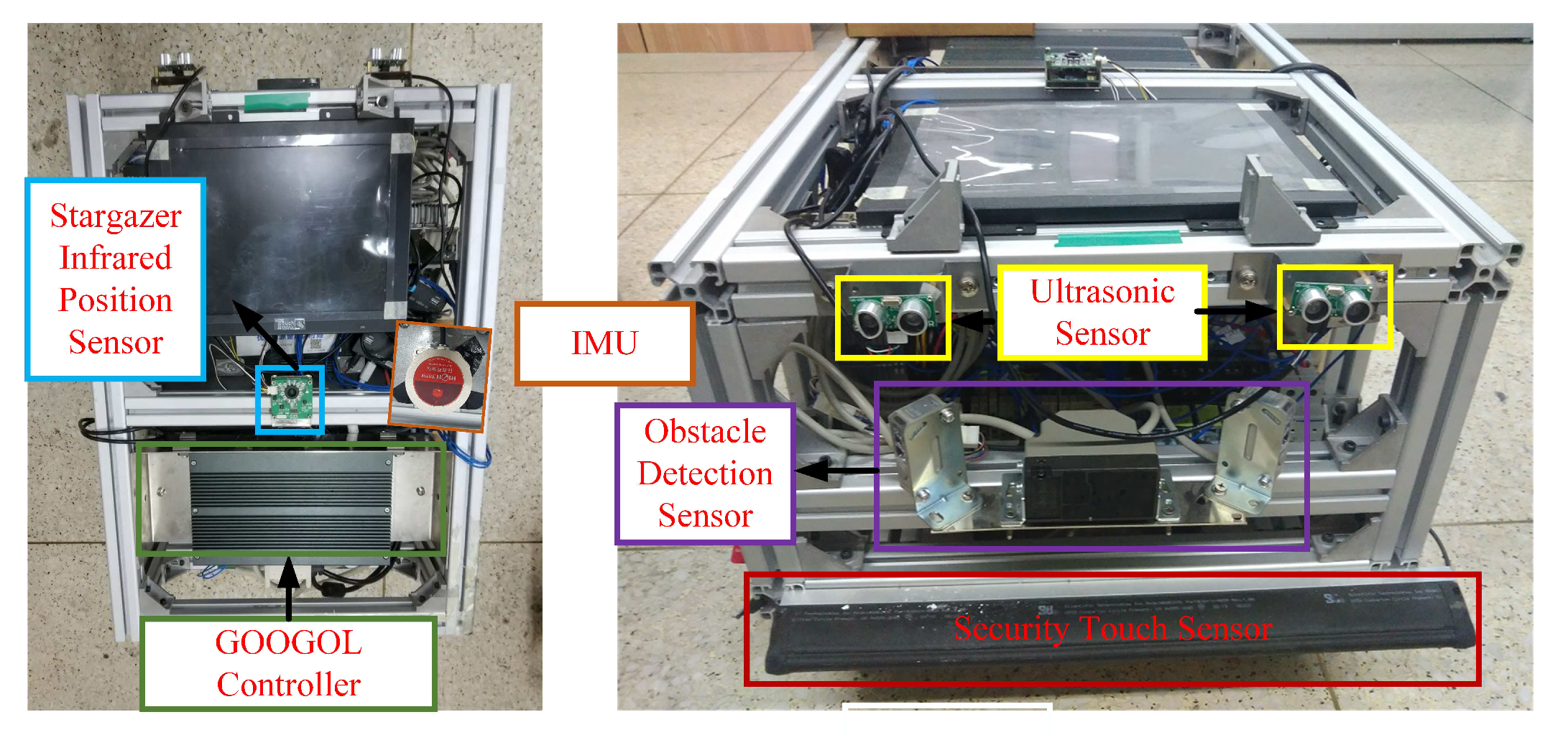
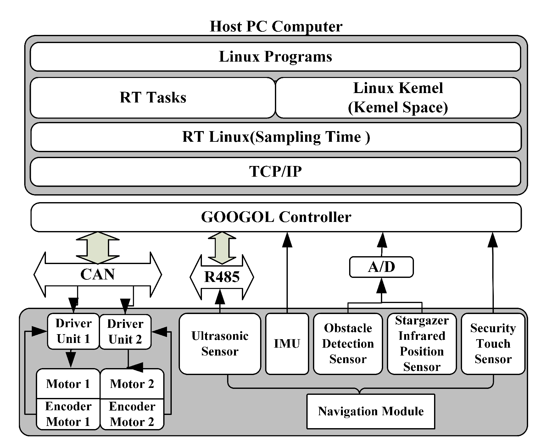
6.1. Experimental Setup

A verification platform is built up to illustrate the ESO-ASMC controller in motion control of WMR with skidding and slipping. The experiment platform consists of two direct motors with absolute rotary encoder, a stargazer infrared position sensor, IMU, obstacle detection sensor, ultrasonic sensor and security touch sensor, as displayed in Figure 5. The IMU is used for collecting the WMR’s current orientation, while the absolute rotary encoder for collecting the position. The specific implementation architecture of WMR is depicted in Figure 6.

In the experimental verification, the linear trajectory is taken as an typical example to conduct the experiment. The WMR with the orientation angle as zero degree starts form the initial location to track the desired trajectory with the orientation angle as 45 degree. The linear trajectory is conducted under three different groups of ground condition: Group A-normal marble ground, Group B-icy ground, and Group C-damp marble ground. The position tracking error is introduced in the inertial coordinate system to evaluate the effects.

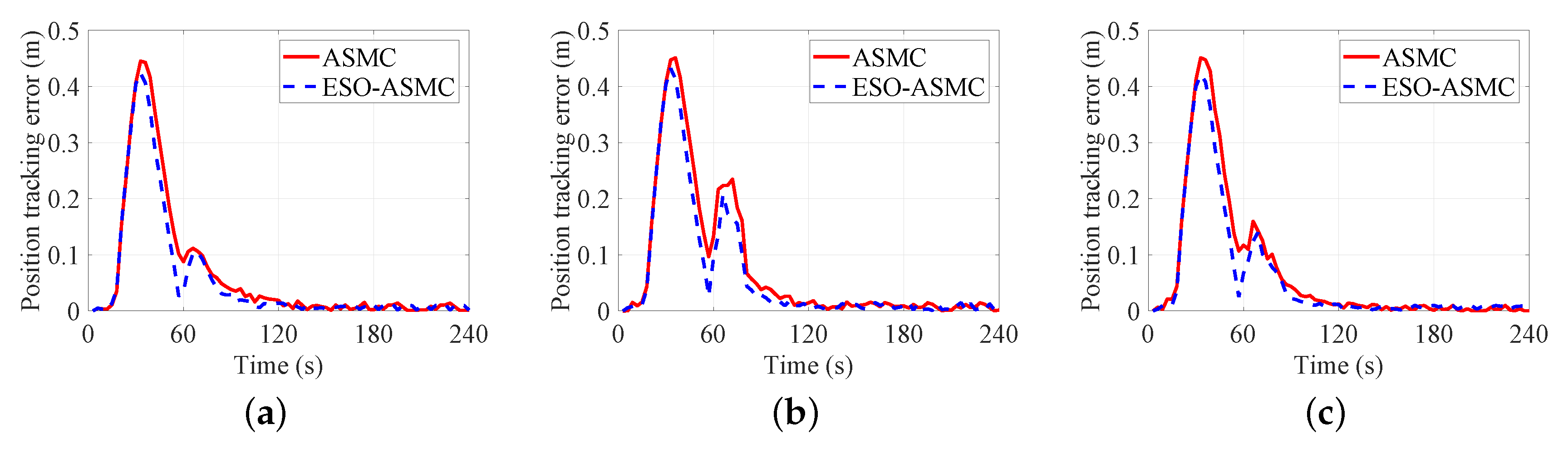
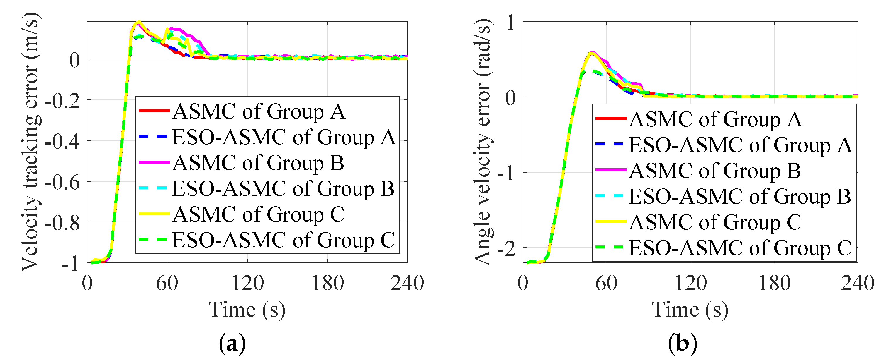
6.2. Experimental Results and Discussion

The experimental results present a similar tendency for the Group A, B, and C, the position tracking precision of the ESO-ASMC scheme is all superior to the ASMC scheme in Figure 7 and

Table 4. Experimental results comparison of ASMC and ESO-ASMC.

Linear Trajectory	RMSE (m)		Max Error (m)		Min Error (m)
	ASMC	ESO-ASMC	ASMC	ESO-ASMC	ASMC	ESO-ASMC
Group A	0.1441	0.1283	0.4452	0.4236	0	0
Group B	0.1509	0.1312	0.4511	0.4323	0	0
Group C	0.1482	0.1296	0.4511	0.4206	0	0

. In the first 60 s, the WMR is required to adjust the orientation angle to track the reference trajectory, thus it leads to the max tracking error in Table 4 for the Group A, B, C. When the slipping and skidding phenomena occurs in the about 60 s, it have negative affects on the real trajectory and velocity. In the Figure 7, it is clearly seen that the max error of the ASMC scheme during slipping-skidding is 0.111 m, 0.235 m, 0.143 m for the Group A, B, C, while the max error of the ESO-ASMC scheme is 0.105 m, 0.207 m, 0.139 m. Despite the experiment with icy ground in Group B makes slipping and skidding phenomena more obvious, the position error in Figure 7b and the RMSE in Table 4 of the Group B present slightly larger comparing with the Group A in Figure 7a and Group C in Figure 7c. Besides, it is noting that the motion of WMR in Group B need similar time to track the reference trajectory in the experiment process. The reason for this phenomenon is that the slipping and skidding as an external decreases the velocity of WMR, thus the controller is required to adjust input component to compensate this deviation due to the wheel slipping and skidding. With the effect of the controller, the min error for both ASMC and ESO-ASMC methods all converge to zero for the Group A, B, C during the whole motion. Although the linear velocity error in Figure 8a and angle velocity tracking error in Figure 8b are a bit larger than the result of Group A and Group C, it suggest that the ESO-ASMC approach in three experimental cases all perform better than the ASMC approach. It indicates that the ESO-ASMC approach has better robustness against disturbance compared with ASMC approach under different working condition. This is consistent with the simulation results. It can be concluded the ESO-ASMC method has certain practicality to the wheel slipping and skidding with the different ground condition and thus can realize the adaptive tracking ability.

7. Conclusions

The present work addresses the trajectory tracking problem of WMR in presence of the wheel skidding and slipping. The kinematic and dynamic model of WMR considering the skidding and slipping phenomenon are derived. The influence of unknown skidding and slipping is regarded as an external disturbance of the WMR system, therefore the extended state observer based adaptive sliding mode control approach is designed to counteract the disturbance and thus improve the path precision performance. The asymptotic stability of the WMR system is proved by Lyapunuov function. Simulation results indicate the ESO-ASMC approach outperforms the ASMC for linear and circular trajectories, i.e., tracking precision, disturbance attenuation. Besides, simulation results also show that the RMSE, max error, and min error for the position tracking are all better than the ASMC. The experimental platform are built, and experiments are conducted to evaluate the ESO-ASMC method under normal, wet, and icy ground. The results suggest that the tracking and disturbance rejection performance of the ESO-ASMC are better than that of the ASMC scheme. Consequently, the ESO-ASMC method possesses great application foreground in the motion control field of mobile manipulator, unmaned ground vehicle, and it could make important contributions to other control problem for the nonlinear system. In our paper, the motion control problem in dynamic level can be achieved just for the differentially driven WMR. In our further research, we will do research about the precise motion control problem of omni-directional four-Mecanum wheel driven mobile robot under skidding and slipping condition.

References

1. Pandey, A. Mobile Robot Navigation in Static and Dynamic Environments using Various Soft Computing Techniques. Ph.D. Thesis, National Institute of Technology Rourkela, Rourkela, India, July 2016. [Google Scholar]
2. Terakawa, T.; Komori, M.; Matsuda, K.; Mikami, S. A novel omnidirectional mobile robot with wheels connected by passive sliding joints. IEEE/ASME Trans. Mechatron. 2018, 23, 1716–1727. [Google Scholar] [CrossRef]
3. Kretzschmar, H.; Spies, M.; Sprunk, C.; Burgard, W. Socially compliant mobile robot navigation via inverse reinforcement learning. Int. J. Robot. Res. 2016, 35, 1289–1307. [Google Scholar] [CrossRef]
4. Quillen, P.; Subbarao, K.; Munoz, J. Guidance and control of a mobile robot via numerical navigation functions and backstepping for planetary exploration missions. In Proceedings of the 2016 AIAA SPACE, Long Beach, CA, USA, 13–16 September 2016. [Google Scholar]
5. Fukao, T.; Nakagawa, H.; Adachi, N. Adaptive tracking control of a nonholonomic mobile robot. IEEE Trans. Robot. Autom. 2000, 16, 609–615. [Google Scholar] [CrossRef]
6. Wu, D.; Cheng, Y.; Du, H.; Zhu, W.; Zhu, M. Finite-time output feedback tracking control for a nonholonomic wheeled mobile robot. Aerosp. Sci. Technol. 2018, 78, 574–579. [Google Scholar] [CrossRef]
7. Chen, J.; Chen, W.E.; Dawson, M.; McIntyre, M. Homography-based visual servo tracking control of a wheeled mobile robot. IEEE Trans. Robot. 2006, 22, 406–415. [Google Scholar] [CrossRef] [Green Version]
8. Mirzaeinejad, H.; Shafei, A.M. Modeling and trajectory tracking control of a two-wheeled mobile robot: Gibbs-Appell and prediction-based approaches. Robotica 2018, 36, 1551–1570. [Google Scholar] [CrossRef]
9. Esmaeili, N.; Alfi, A.; Khosravi, H. Balancing and trajectory tracking of two-wheeled mobile robot using backstepping sliding mode control: Design and experiments. J. Intell. Robot. Syst. 2017, 87, 601–613. [Google Scholar] [CrossRef]
10. Asif, M.; Khan, M.J.; Cai, N. Adaptive sliding mode dynamic controller with integrator in the loop for nonholonomic wheeled mobile robot trajectory tracking. Int. J. Control 2014, 87, 964–975. [Google Scholar] [CrossRef]
11. Peng, S.; Shi, W. Adaptive fuzzy integral terminal sliding mode control of a nonholonomic wheeled mobile robot. Math. Probl. Eng. 2017, 2017, 1–12. [Google Scholar] [CrossRef]
12. Ding, L.; Li, S.; Gao, H.; Chen, C.; Deng, Z. Adaptive partial reinforcement learning neural network-based tracking control for wheeled mobile robotic systems. IEEE Trans. Syst. Man Cybern. Syst. 2018, 1–12. [Google Scholar] [CrossRef]
13. Yang, H.; Fan, X.; Shi, P.; Hua, C.C. Nonlinear control for tracking and obstacle avoidance of a wheeled mobile robot with nonholonomic constraint. IEEE Trans. Control Syst. Technol. 2016, 24, 741–746. [Google Scholar] [CrossRef]
14. Huang, D.; Zhai, J.; Ai, W.; Fei, S. Disturbance observer-based robust control for trajectory tracking of wheeled mobile robots. Neurocomputing 2016, 198, 74–79. [Google Scholar] [CrossRef]
15. Hwang, E.J.; Kang, H.S.; Hyun, C.H.; Park, M. Robust backstepping control based on a Lyapunov redesign for skid-steered wheeled mobile robots. Int. J. Adv. Robot. Syst. 2013, 10, 26. [Google Scholar] [CrossRef]
16. Wang, D.; Low, C.B. Modeling and analysis of skidding and slipping in wheeled mobile robots: Control design perspective. IEEE Trans. Robot. 2008, 24, 676–687. [Google Scholar] [CrossRef]
17. Low, C.B.; Wang, D. GPS-based path following control for a car-like wheeled mobile robot with skidding and slipping. IEEE Trans. Control Syst. Technol. 2008, 16, 340–347. [Google Scholar]
18. Low, C.B.; Wang, D. GPS-based tracking control for a car-like wheeled mobile robot with skidding and slipping. IEEE/ASME Trans. Mechatron. 2008, 13, 480–484. [Google Scholar]
19. Dixon, W.E.; Dawson, D.M.; Zergeroglu, E. Robust control of a mobile robot system with kinematic disturbances. In Proceedings of the IEEE International Conference on Control Applications, Anchorage, AK, USA, 27 September 2000; pp. 437–442. [Google Scholar]
20. Gonzalez, R.; Fiacchini, M.; Alamo, T.; Guzman, J.L.; Rodriguez, F. Adaptive control for a mobile robot under slip conditions using an LMI-based approach. Eur. J. Control 2010, 16, 144–155. [Google Scholar] [CrossRef]
21. Cui, M.; Sun, D.; Liu, W.; Zhao, M.; Liao, X. Adaptive tracking and obstacle avoidance control for mobile robots with unknown sliding. Int. J. Adv. Robot. Syst. 2012, 9, 171. [Google Scholar] [CrossRef]
22. Gao, H.; Song, X.; Ding, L.; Xia, K.; Li, N.; Deng, Z. Adaptive motion control of wheeled mobile robot with unknown slippage. Int. J. Control 2014, 87, 1513–1522. [Google Scholar] [CrossRef]
23. Li, S.; Ding, L.; Gao, H.; Chen, C.; Liu, Z.; Deng, Z. Adaptive neural network tracking control-based reinforcement learning for wheeled mobile robots with skidding and slipping. Neurocomputing 2018, 283, 20–30. [Google Scholar] [CrossRef]
24. Chen, M. Disturbance attenuation tracking control for wheeled mobile robots with skidding and slipping. IEEE Trans. Ind. Electron. 2016, 64, 3359–3368. [Google Scholar] [CrossRef]
25. Kang, H.S.; Kim, Y.T.; Hyun, C.H.; Park, M. Generalized extended state observer approach to robust tracking control for wheeled mobile robot with skidding and slipping. Int. J. Adv. Robot. Syst. 2013, 10, 155. [Google Scholar] [CrossRef]
26. Kang, H.S.; Hyun, C.H.; Kim, S. Robust tracking control using fuzzy disturbance observer for wheeled mobile robots with skidding and slipping. Int. J. Adv. Robot. Syst. 2014, 11, 75. [Google Scholar] [CrossRef]
27. Chen, C.; Gao, H.; Ding, L.; Li, W.; Yu, H.; Deng, Z. Trajectory tracking control of WMRs with lateral and longitudinal slippage based on active disturbance rejection control. Robot. Auton. Syst. 2018, 107, 236–245. [Google Scholar] [CrossRef]
28. Ding, Z. Consensus disturbance rejection with disturbance observers. IEEE Trans. Ind. Electron. 2015, 62, 5829–5837. [Google Scholar] [CrossRef]
29. Xu, B. Disturbance observer-based dynamic surface control of transport aircraft with continuous heavy cargo airdrop. IEEE Trans. Syst. Man Cybern. Syst. 2016, 47, 161–170. [Google Scholar] [CrossRef]
30. Jingqing, H. The extended state observer of a class of uncertain systems. Control Decis. 1995, 10, 85–88. [Google Scholar]
31. Chen, W.H.; Yang, J.; Guo, L.; Li, S. Disturbance-observer-based control and related methods-An overview. IEEE Trans. Ind. Electron. 2015, 63, 1083–1095. [Google Scholar] [CrossRef]
32. Castillo, A.; Garcia, P.; Sanz, R.; Albertos, P. Enhanced extended state observer-based control for systems with mismatched uncertainties and disturbances. ISA Trans. 2018, 73, 1–10. [Google Scholar] [CrossRef] [Green Version]
33. Mallavalli, S.; Fekih, A. Adaptive fault tolerant control design for actuator fault mitigation in quadrotor UAVs. In Proceedings of the IEEE Conference on Control Technology and Applications, Copenhagen, Denmark, 21–24 August 2018; pp. 193–198. [Google Scholar]
34. Huang, Y.J.; Kuo, T.C.; Chang, S.H. Adaptive sliding-mode control for nonlinearsystems with uncertain parameters. IEEE Trans. Syst. Man Cybern. Part B Cybern. 2008, 38, 534–539. [Google Scholar] [CrossRef]
Figure 1. Overview of the differentially driven wheeled mobile robot (WMR).
Energies 12 03305 g001
Figure 2. Block diagram of control method.
Energies 12 03305 g002
Figure 3. Linear trajectory tracking for WMR considering skidding and slipping. (a) Trajectory tracking. (b) Position tracking error. (c) Linear velocity tracking. (d) Angle velocity tracking. (e) Velocity tracking error. (f) Control input. ESO = extended state observer; ASMC = adaptive sliding mode controller.
Energies 12 03305 g003
Figure 4. Circular trajectory tracking for WMR considering skidding and slipping. (a) Trajectory tracking. (b) Position tracking error. (c) Linear velocity tracking. (d) Angle velocity tracking. (e) Velocity tracking error. (f) Control input.
Energies 12 03305 g004
Figure 5. Experiment platform of WMR.
Energies 12 03305 g005
Figure 6. Implementation architecture of WMR.
Energies 12 03305 g006
Figure 7. Position tracking errors. (a) Group A. (b) Group B. (c) Group C.
Energies 12 03305 g007
Figure 8. Velocity tracking errors. (a) Linear velocity tracking error. (b) Angle velocity tracking error.
Energies 12 03305 g008