1. Introduction
Transmission-line protection is critical to power system security. High speed and selective isolation of faults in transmission lines help to improve the reliability of the power supply. Accuracy in locating permanent faults is also important.
The most widely used fault-detection algorithms calculate the fundamental frequency of current and voltage waveforms and then impedance is determined. Although this solution features a low computational cost and high reliability, it is time-consuming (at least one cycle). As lines are repaired by crews, a precise fault location minimizes repair time and benefits the security and quality of the supply.
The accuracy of the impedance method for fault location is affected by fault resistance, the mutual coupling effect and vague line-parameter knowledge [
1]. Parameter-free fault-location algorithms provide more accurate results [
2,
3].
When a fault happens, transients are generated and propagate through the transmission line. Fault information is included in the waves traveling toward both ends. Furthermore, traveling wave-based methods can provide accurate fault location in shorter time frames [
4,
5], which also make them suitable for DC systems [
6].
Acquiring the arrival time of the traveling wave is difficult, but it can be done accurately using wavelet transform (WT) [
7,
8]. These methods can be single-ended [
9] or double-ended [
10]. In the first case, data are independent from the communication equipment and also make it possible to avoid the complexities of synchronization between terminals [
11].
WT is effective for analyzing voltage [
12] and current signals associated with faults both in the frequency and time domain [
13]. WT is merged with other methods, such as artificial neural networks [
14], probabilistic neural networks on transmission lines with FACTS [
15], least-squares method [
11], extreme learning machine (ELM) [
16] or support vector machine [
17], where WT is normally used to detect and classify the fault, and then the cited techniques estimate fault location.
Wavelet-based methods are characterized by their speediness and accuracy in fault detection and location; however, they may not be successful for fault location with a low inception angle [
18,
19]. For unsymmetrical faults to earth with a low fault-inception angle, aerial-mode coefficients may have low values; in this case, they are masked by noise. To address this issue, a fault detection and location scheme based on the zero-mode coefficient analysis was proposed in [
20] but its precision for these faults was low (about 5%). Additionally, due to limitations imposed by the current sampling frequency, faults occurring close to the relay location cannot be located using the WT method.
Location methods based on response to impulse injection are proposed in [
21,
22]. In both cases, the methods are applied to distribution systems. In [
21] the location method is based on calculating the input impedance matrix for the location of high-impedance faults in overhead distribution lines. In [
22], the fault location is based on detecting the instant when pre-fault and fault images diverge.
In this paper, a new accurate fault-location algorithm is proposed. The algorithm, based on the WT, uses the aerial mode and zero mode of the current wave to detect faults. WT is also used to locate the fault, except for single-line-ground (SLG) faults with low inception angle and when faults occur close to the relay; the proposed half-sine method is applied in these cases. When a fault is detected, 100 kHz half-sine voltage waveforms are injected into each phase of the transmission line and the response given by the fault point is measured. The fault distance is calculated accurately from the time elapsed between the half-sine injection instant and the response derivative maximum.
2. WT with Multiresolution Analysis
The discrete wavelet transform (DWT) decomposes a sampled signal
f(
t) into a set of wavelets
ψ:
where the integers
k and
j are the translation and dilation factors, respectively, and
the
DWT coefficients in the wavelet basis considered.
Alternatively, multiresolution analysis (MRA) provides a different time-and-frequency resolution at each level of analysis. MRA employs two sets of functions (scaling functions
φ(
t) and wavelet functions
ψ(
t)), which allow the sampled signal
f(
t) to expand thus:
where
is the approximation coefficients and
the detail coefficients, which can be calculated in terms of the scaling and wavelet basis:
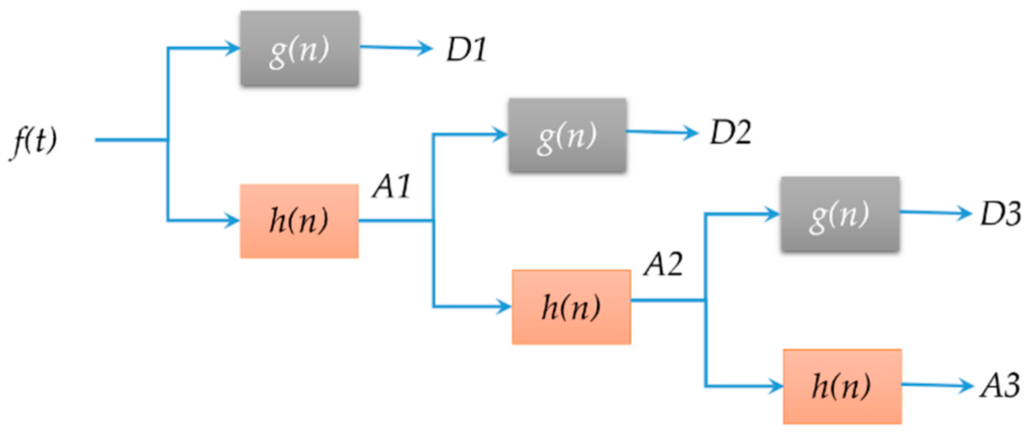
MRA builds a wavelet decomposition tree as shown in
Figure 1. At each level, the signal is decomposed by applying successive pairs of low-pass (
h(
n)) and high-pass (
g(
n)) filters. After each filtering, half of the samples are eliminated and a level of decomposition is achieved at each end row; detail coefficients
D1,
D2,
D3 and approximation coefficients
A3 are obtained as a result. It allows both time and frequency information to be extracted simultaneously, even though the resolution differs; consequently, high time resolution is achieved for lower frequencies. Once the current fault transients are decomposed into their modal components (
Section 5), the MRA of these signals allow to obtain WT coefficients of the aerial mode and zero mode current which are used to detect faults. For unsymmetrical faults to earth, zero-mode coefficients (i
0) are considered. In the other cases, aerial-mode currents (i
α, i
β) are considered. WT is also used to locate the fault, except for single-line-ground (SLG) faults with low inception angle and when faults occur close to the relay; the proposed half-sine method is applied in these cases.
3. Half-Sine Method
The transient response to a disturbance in the transmission system is obtained by solving the differential equations governing signal propagation:
where the column vectors [
V(
t)] and [
i(
t)] represent the voltages and currents along the conductors, and [
R], [
L], [
G] and [
C] represent the per-unit-length resistance, inductance, conductance, and capacitance, respectively. The solution to these differential equations is the sum of an incident and a reflected wave. In time domain analysis, the response wave
R(
t) is the convolution of the incident wave
Vin(
t) with the impulse response
h(
t), which can be expressed in matrix notation as follows
where [
R(
t)] and [
Vin(
t)] are two sequences of n samples, and [
h(
t)] is a cyclic convolution matrix (nxn).
In the proposed method, a half-sine (per phase) is injected into the transmission line under normal conditions, before the fault event. The half-sine
Hs is defined as
where
u(
t) is the unit step function and
f the frequency.
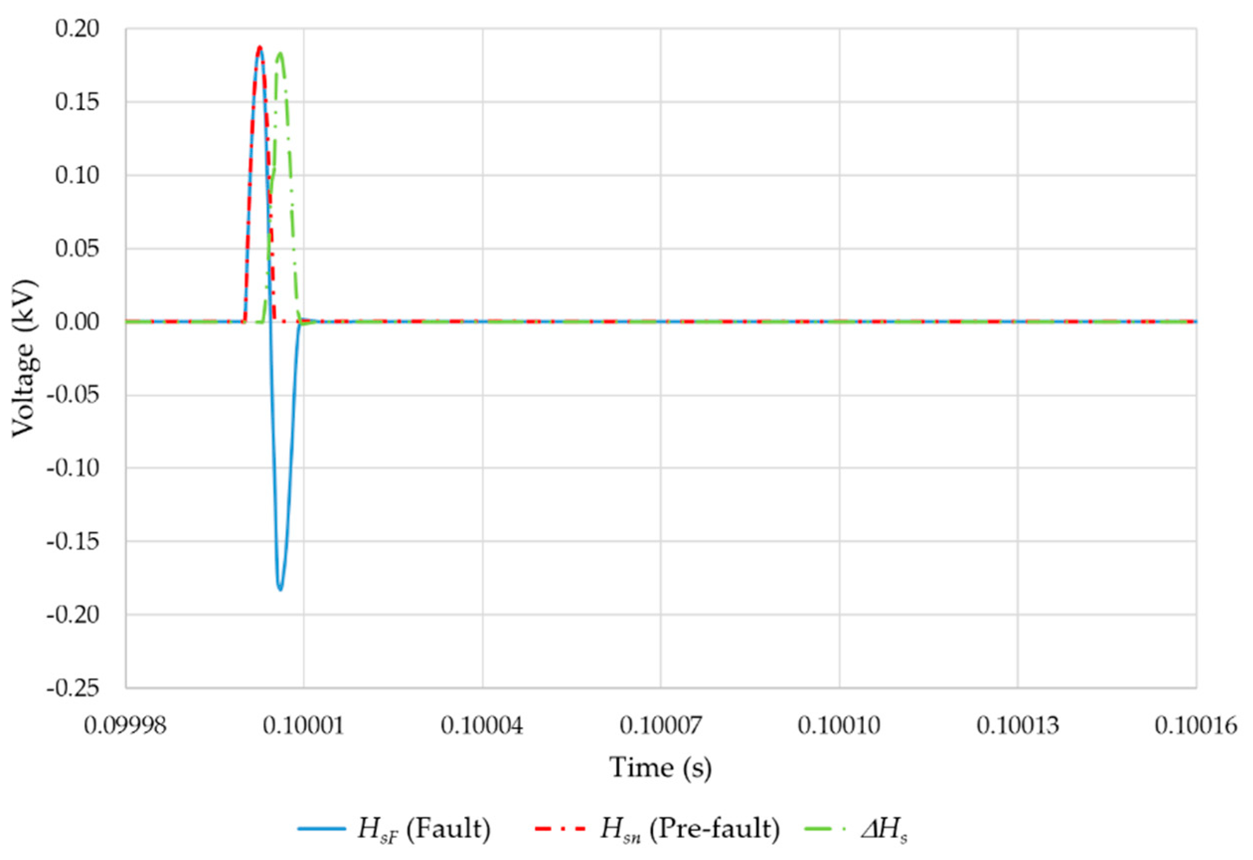
After fault detection, a new half-sine (Hs) is injected, which propagates along the line until it reaches the fault point, where it is reflected back.
The difference (∆
Hs) between the signals measured when half-sines are injected in normal conditions (
Hsn) and in fault conditions (
HsF) is given by:
The travel time to the fault point (Δt), and the propagation speed (v), taking the instants when half-sines are injected as a time reference, allow us to calculate the distance to the fault (d) easily.
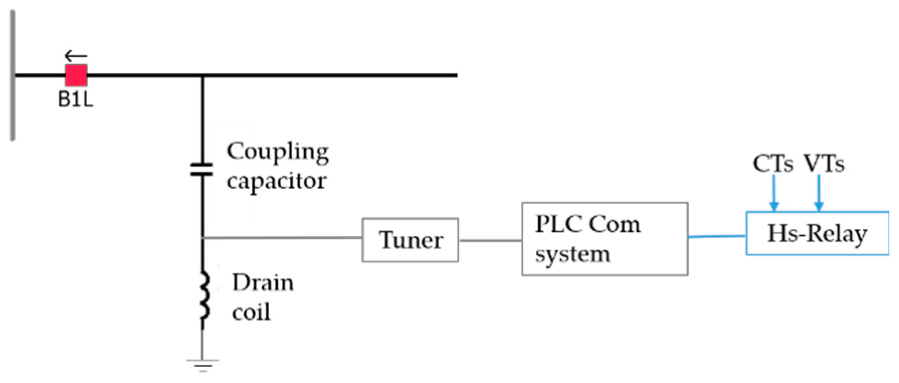
To inject the half-sine, the coupling capacitors of a PLC (power-line communication) connection can be used as shown in
Figure 2, where the injection is done by means of the fault locator device (
Hs-relay). The coupling filter and the capacitance of the coupling capacitors are a broad band-pass filter matching the transmission-line surge impedance with the device impedance. To keep the bandwidth as wide as possible and to reduce the loss of energy on the transmission, the capacitance in use usually varies from 1 to 50 nF. PLCs are in common use, which makes the approach more applicable.
4. Modeled Power System
The power system considered here is the 132-kV system shown in
Figure 3, which has been modeled in PSCAD/EMTDC [
23]. The
Hs-relay analysed in this study is installed at the line position B1L at G1. The transmission-line lengths are 100 km for the transmission line TL1 and 120 km for the transmission line TL2 and, in both cases, the frequency-dependent phase model is applied. Harmonic distortion in voltage waveform is also considered; the expected THD in voltage waveform (THDV) must be lower than 2.5% for normal operations, and for conditions lasting less than one hour, this limit may be exceeded by 50%. Therefore, the THDV is set to a value of 3.75%.
The electrical networks connected to the buses G1 and G2 are represented by their respective Thévenin equivalent voltage and impedance (
Figure 3).
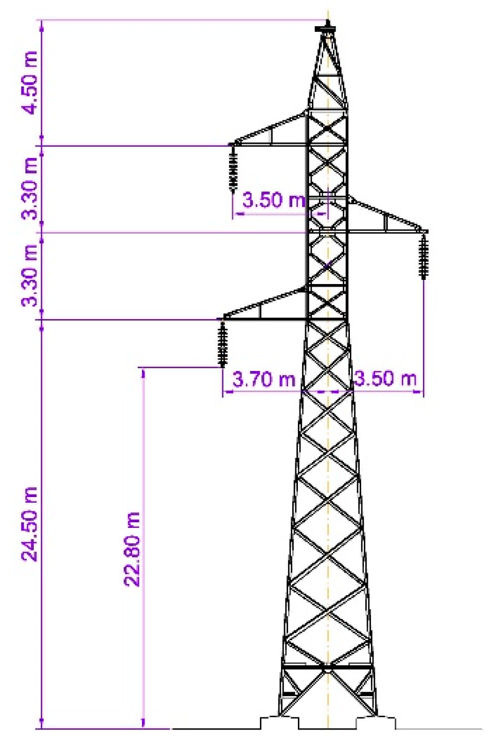
Figure 4 shows the transmission tower dimensions.
The propagation speed for aerial modes and for the earth mode is calculated by:
where
L1 and
C1 are the positive sequence inductance and capacitance, and
L0 and
C0 are the zero sequence inductance and capacitance whose values are shown in
Table 1.
These values of L0 and C0, and the zero sequence speed v0 given by Equation (11), have been calculated considering the ground as a perfect conductor, which is true for seawater; however, the value of ground resistivity will vary for different soil types and, while C0 is constant, L0 and, consequently, v0 are affected by this parameter.
5. Fault Detection and Location Algorithm
A flowchart of the proposed fault detection and location algorithm is shown in
Figure 5.
5.1. Fault Detection
Fault inception gives rise to a variation of current modes, which allows detection schemes based on the WT to determine whether faults are present. Detection schemes based on WT use the aerial-mode current. However, when the fault-inception angle is close to zero, the fault signal detected is weak and can be masked by noise. To avoid this drawback, fault detection can be improved by considering zero-mode coefficients, which provide more relevant information and appreciable magnitudes with fault-inception angles close to the zero-crossing region. In a high-impedance grounded distribution network, the accuracy of this detection method would drop due to problems such as a weak fault signal, noise or unbalanced operation, and other techniques should, therefore, be considered [
21]. However, this is not the case of (usually solidly) grounded transmission systems.
The current fault transients are decomposed into their modal components and, to improve fault detection, both aerial- and zero-mode coefficients are employed for fault detection. For unsymmetrical faults to earth, zero-mode coefficients are considered. In the other cases, aerial-mode currents are considered.
Table 2 shows the current modes considered to detect the fault type (single-line-to-ground (SLG), line-to-line (LL), line-to-line-to-ground (LLG) or three-phase faults (3L/3LG)).
5.2. Wavelet Analysis
Modal transformation allows a three-phase coupled line to be decomposed into three independent propagation modes. Out of the various modal transformation methods, Clarke transformation is employed to calculate the modal components of currents:
where
i0 is the zero or earth mode, and
iα,
iβ are the aerial modes of the current.
The MRA of a signal provides WT coefficients; the absolute local maximum values of these coefficients and the instants of occurrence (i.e., the arrival times of the traveling waves from the fault point to the substation) are obtained using wavelet modulus maxima (WMM).
Figure 6 shows the result of applying WMM to the detail coefficients.
The mother wavelet type, as well as the number of decomposition scales, may differ from one application or condition to another and, therefore, cannot be generalized to all cases. Several wavelet families with a variety of vanishing moments, such as Haar, Daubechies (db), Symlets, Coiflets, Biorthogonal, Reverse Biorthogonal and Discrete Meyer, were tested to select the most suitable mother wavelet. According to the results, and considering Daubechies family properties in fault-location applications and their low computational cost, db3 wavelet was selected as the mother wavelet.
Applying WMM allows us to clearly identify the wave peaks, and, therefore, fault distance is determined as follows:
where
d_wt is the estimated distance to fault,
t2 − t1 is the time difference between two consecutive maximum values of WT coefficients and v is the propagation speed through the line or ground.
The propagation speed in aerial modes is calculated from positive sequence parameters by means of Equation (10). For SLG faults with a low inception angle, aerial-mode coefficients are not effective. The zero mode is not used in the proposed algorithm because fault location using zero-mode coefficients leads to errors. Measuring zero-mode velocity with enough accuracy is difficult as ground resistivity varies along the line.
When SLG faults occur with a low inception angle, the algorithm applies the half-sine H’s method, as explained below.
5.3. Hs and H’s Methods
The fault-locator device injects Hs signals and registers the response of the network under normal conditions, allowing the fault locator to detect any irregularity in the transmission line.
5.3.1. H’s Method
When a fault is detected, Hs are injected in each phase of the transmission line and recorded. Therefore, the algorithm calculates the signal ∆Hs, given by Equation (9). The maximum of ∆Hs can be used to determine the time ΔtHsF elapsed between the instant a Hs signal is injected and the reception of the reflected signal when the fault has happened, taking the instants when Hs are injected as a time reference. Finally, the distance to the fault (dHsF) is obtained as follows
For faults near to a substation, both high and low frequency
Hs allow for fault location. For long-distance faults and high-frequency
Hs, the signal is affected by attenuation. However, for low frequency
Hs there is also a clear signal deformation and a deviation of the maximum (
Figure 7), which finally results in greater inaccuracies in the fault location.
Signals are sampled with a frequency of 1.7 MHz. Hence, a 5 kHz
Hs, which has a duration of 0.1 ms, is described by 170 samples. However, in a 100 kHz
Hs (duration of 5 μs) only 8 points are sampled. As can be seen in
Figure 8, compared with the 5 kHz
Hs, the 100 kHz,
Hs is of shorter duration and, consequently, the attenuation affects the 100 kHz
Hs amplitude without causing a deviation of the signal maximum, as happens for a low frequency
Hs.
5.3.2. H’s Method
A preferable alternative to the detection of the maximum in the
Hs method is to consider the time derivative of ∆
Hs which can be expressed as the convolution of
H’s and the variation of the system impulse response (Δ
nF) under fault compared with normal conditions
where
H’s starts at a maximum value making it easier to locate the distance to the fault (
dH’sF). Likewise, it is easier to inject a sine than a cosine, whose difficulty is equivalent to generating an ideal step. In
Figure 9,
H’s is compared with
Hs.
5.3.3. Comparison of Hs and H’s Methods
Table 3 shows a comparison of results obtained using the aforementioned methods for a long-distance fault (100 km, at the end of the line) and considering a constant soil resistivity of 200 Ω∙m:
5-kHz Hs: The fault distance is calculated measuring the time interval (dHsF) between the signal maximum ∆Hs and the time reference (signal injection instant), when a Hs of 0.1 ms duration is applied.
5-kHz H’s: The distance (dH’sF) is obtained by measuring the time between the derivative signal of a 5-kHz Hs and the time reference.
100-kHz Hs and 100-kHz H’s: The fault distance dH’sF is calculated as before but with half-sines of 5 μs duration.
It can be noticed that the H’s method shows good results, especially for high-frequency half-sines. Therefore, to improve accuracy, the fault distance is evaluated using a 100-kHz half-sine, which is a frequency compatible with PLC equipment that can operate over a frequency band up to 500 kHz.
6. Discussion and Results
6.1. Discussion
Although WT methods offer high accuracy in fault location, a drawback associated with this method is that faults close to the substation cannot be located due to the limitation of sampling frequency.
To ensure an accurate fault location, the time difference between two consecutive peaks of the WT coefficients is considered to be, at least, twice the period of the applied WT. Therefore, in the case of this fault locator (current signals are sampled at 1.7 MHz), 2 km is the threshold distance (Blind_d) from which the WT method gives accurate fault-location estimation, and below this distance there is a blind zone. To overcome this shortcoming, the sampling frequency could be increased, but that would make it too expensive. The proposed algorithm tackles this drawback by applying the H’s method for calculating the fault distance with single-phase-to-ground faults and with low inception-angle faults, achieving good accuracy in both cases.
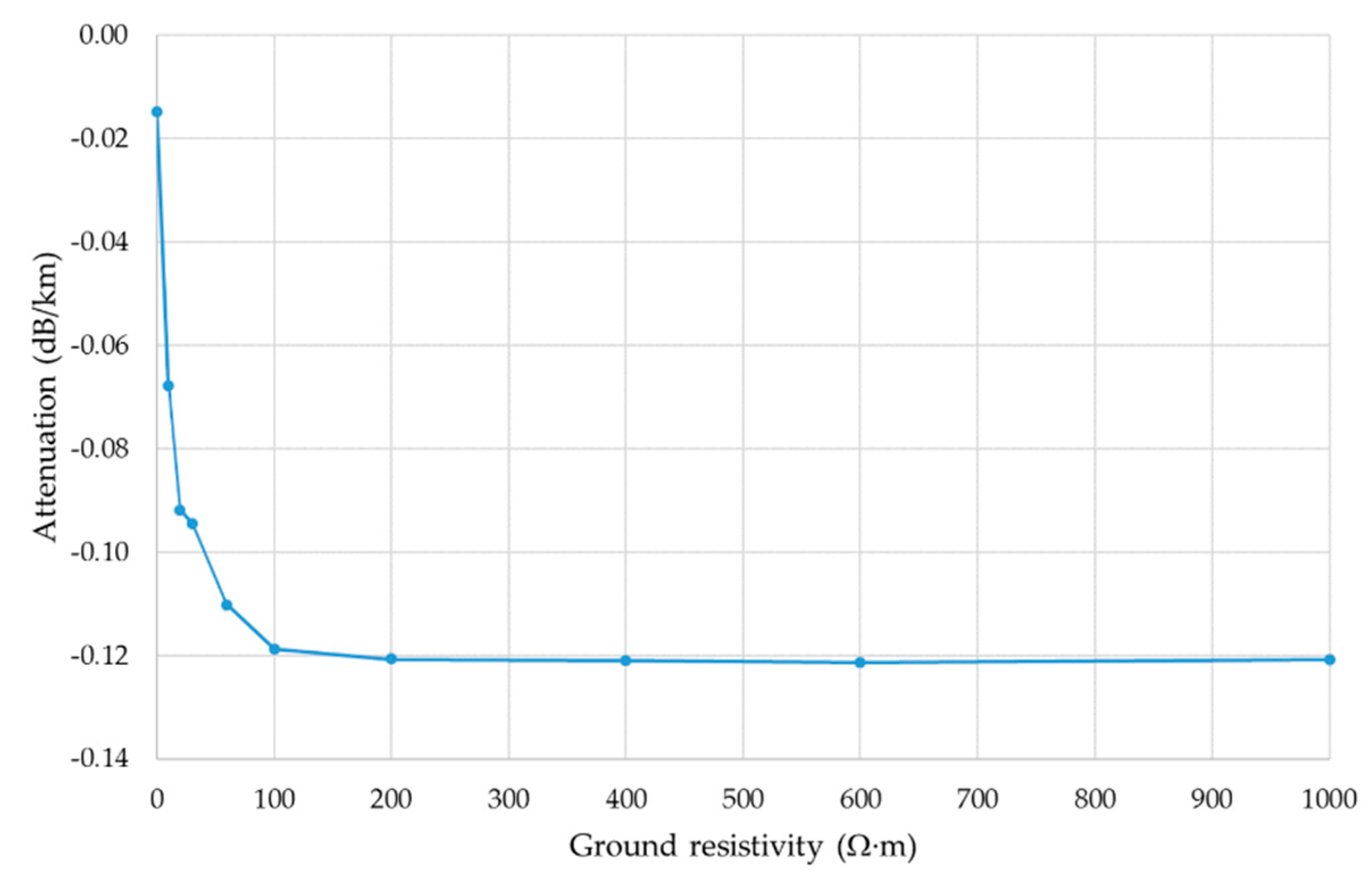
In overhead lines, signals lose energy as they are transmitted. Attenuation per unit length increases with frequency due to the skin effect, but it is also affected by ground resistivity (
ρ) [
4]. In propagation in overhead lines with ground return, the series impedance per unit length is the sum of the series impedances considering ground as a perfect conductor and of the ground impedance integral [
24], which is evaluated in PSCAD through direct numerical integration. Alternatively, the ground impedance integral can be estimated by an analytical approximation [
25,
26]. If ground is a perfect conductor (
ρ ≈ 0 Ω∙m), the attenuation is negligible. For low values of
ρ (<100 Ω∙m), the attenuation rises rapidly with increasing
ρ, and, from this point (
ρ = 100 Ω∙m), it remains almost constant as shown in
Figure 10. The ground effect return affects the injected half-sines as the length of the line increases; therefore, it will determine the half-sine amplitude.
6.2. Simulation Results
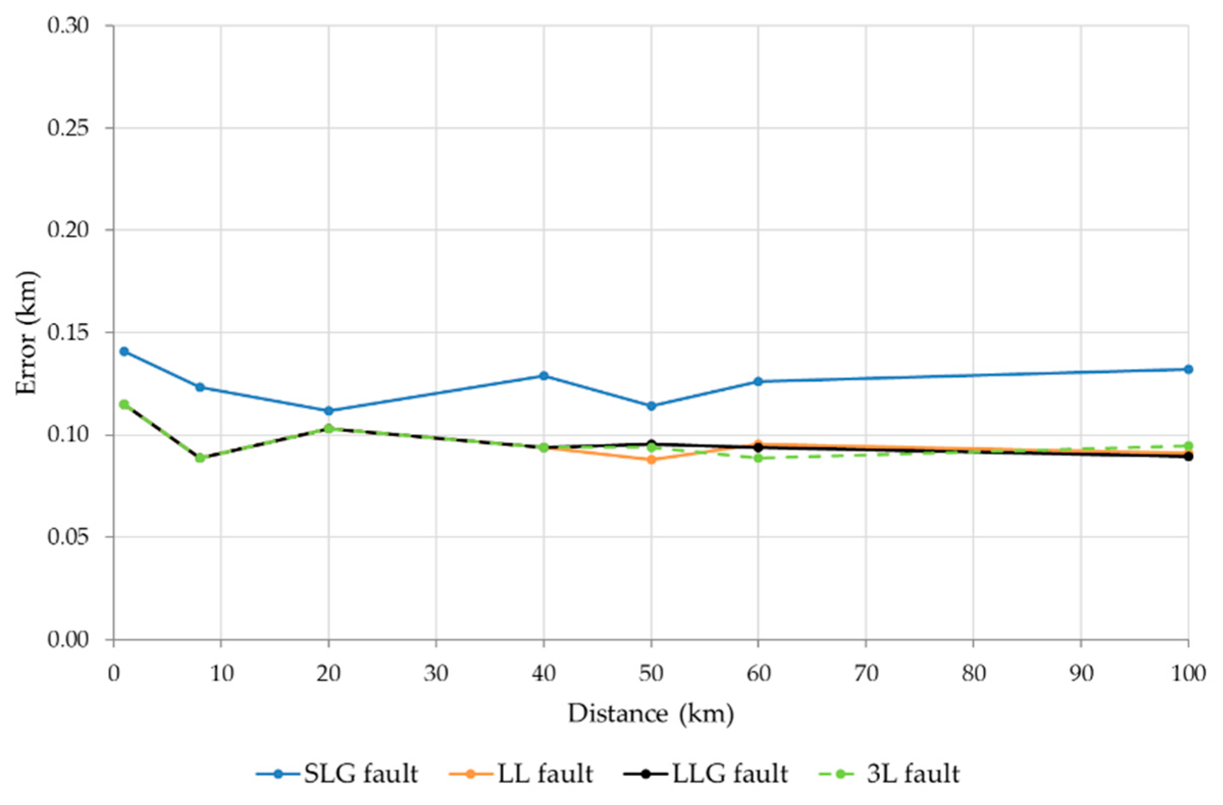
The algorithm performance is evaluated by varying fault resistance, location, and fault type on the power system of
Figure 3.
Figure 11 and
Figure 12 show the error in fault distance estimation for single-line-ground (SLG), double-line-to-ground (LLG), line-to-line (LL) and three-phase (3L) faults, varying fault location (1, 8, 20, 30, 40, 50, 60 and 100 km). It should be noted that these errors are almost insensitive to different fault types, being slightly higher for SLG faults.
Figure 13 depicts the error in fault distance estimation for different fault locations (1, 8, 20, 40, 50, 60 and 100 km) and fault resistance values (between 0 Ω and 150 Ω), in case of SLG faults.
For faults close to the bus, below the threshold distance
Blind_d and for the sampling frequency considered, the error (
Table 4) is lower than 133 m (0.13%) and independent of the angle of inception, fault resistance or ground resistivity. For longer distances, the maximum relative error detected is 0.14%, which is obtained for a fault resistance value of 150 Ω when an SLG fault is applied. These results were obtained considering the worst harmonic distortion and inception angle (0°) conditions.
Figure 14 shows how the error for different location faults is not affected by the inception angle which is varied between 0° and 270°. Additionally, these results are not altered when ground resistivity values vary (between 0 and 10,000 Ω∙m), as can be noticed in
Figure 15. Ground resistivity just affects waveform attenuation and, for sufficient high-frequency half-sine, the impact is negligible.
In
Table 5 the proposed method is compared with several methods: a traditional distance algorithm (DFFT distance algorithm) [
27], a distance relaying scheme based on the current phase jump behaviour during fault conditions to improve the apparent impedance estimated (DFFT distance algorithm + JCF) [
27], a fault location method based on time difference of arrival of ground-mode and aerial-mode traveling waves [
4], a wavelet-based method [
20] and the proposed method. The comparison shows that the proposed method has better accuracy with respect to the traditional methods described in [
20] and [
27]. The proposed algorithm accuracy is obtained even for faults close to the bus (<2%), low inception angles and it is independent of the soil resistivity value.
Finally, overreach, as a common cause of incorrect operation, was considered. To identify external faults, a reference could be registered during line energization with the remote terminal open. However, when a close fault happens in the adjacent line TL2 (
Figure 3) and measuring errors are considered, there could be a small probability of incorrect operation. A time-delayed zone could be defined to solve this problem, but the protection should, nevertheless, be fast, and any intentional time delay should be avoided. There is a better alternative, the reception of the
Hs signal from the remote end can be used to block the trip. The proposed scheme will provide selective and fast clearance of faults. The response time of the proposed algorithm to detect faults is lower than 0.5 ms.
7. Conclusions
An accurate fault-location scheme for transmission lines is presented based on single-ended measurements.
Faults are detected by a wavelet multi-resolution analysis of the current transients. Aerial current modes are used, and zero modes are considered to improve fault detection when fault-inception angles are close to zero.
Fault location is also based on the wavelet analysis, except for faults close to the bus and fault-inception angles near to zero for SLG faults. In such cases, the fault locator employs the H’s method to improve accuracy. In the proposed H’s method, the fault distance is calculated by measuring the difference between the time when a 100-kHz half-sine signal is sent and the time when the derivative response is received.
The proposed algorithm was checked considering harmonic distortion and varying fault resistance, ground resistivity, location and inception angle. According to these results, the distance location can be determined with an accuracy lower than 150 m in all the cases.
Author Contributions
S.M.A. and M.G.-G. performed the simulations and wrote the paper. A.M. contributed with the wavelet algorithm part and valuable comments and corrections. All authors discussed the results and commented on the manuscript at all stages.
Funding
This research was funded by Spanish Economy, Industry and Competitiveness Ministry and by European Regional Development Fund (ERDF), grant number RTC-2016-5234-3, in the frame of the Project MHiRED “New technologies for wind-photovoltaic hybrid mini networks managed with storage in connection to the grid and with synchronous support in off-grid operation”.
Acknowledgments
The authors wish to thank the technical support from the Research Group on Renewable Energy Integration of the University of Zaragoza (funded by the Government of Aragon).
Conflicts of Interest
The authors declare no conflict of interest.
References
- Das, S.; Santoso, S.; Gaikwad, A.; Patel, M. Impedance-Based Fault Location in Transmission Networks: Theory and Application. IEEE Access 2014, 2, 537–557. [Google Scholar] [CrossRef]
- Wang, C.; Yun, Z. Parameter-Free Fault Location Algorithm for Distribution Network T-Type Transmission Lines. Energies 2019, 12, 1534. [Google Scholar] [CrossRef]
- Dobakhshari, A.S. Noniterative Parameter-Free Fault Location on Untransposed Single-Circuit Transmission Lines. IEEE Trans. Power Deliv. 2017, 32, 1636–1644. [Google Scholar] [CrossRef]
- Liang, R.; Yang, Z.; Peng, N.; Liu, C.; Zare, F. Asynchronous Fault Location in Transmission Lines Considering Accurate Variation of the Ground-Mode Traveling Wave Velocity. Energies 2017, 10, 1957. [Google Scholar] [CrossRef]
- Guzmán, A.; Kasztenny, B.; Tong, Y.; Mynam, M.V. Accurate and Economical Traveling-Wave Fault Locating Without Communications. In Proceedings of the 2018 Texas A&M Conference for Protective Relay Engineers, College Station, TX, USA, 26–29 March 2018. [Google Scholar]
- Zhang, S.; Zou, G.; Huang, Q.; Gao, H. A Traveling-Wave-Based Fault Location Scheme for MMC-Based Multi-Terminal DC Grids. Energies 2018, 11, 401. [Google Scholar] [CrossRef]
- Robertson, D.C.; Camps, O.I.; Mayer, J.S.; Gish, W.B. Wavelets and Electromagnetic Power System Transients. IEEE Trans. Power Deliv. 1996, 11, 1050–1058. [Google Scholar] [CrossRef]
- Hasheminejad, S.; Seifossadat, S.G.; Razaz, M.; Joorabian, M. Ultra-High-Speed Protection of Transmission Lines Using Traveling Wave Theory. Electr. Power Syst. Res. 2016, 132, 94–103. [Google Scholar] [CrossRef]
- Zhang, G.; Shu, H.; Lopes, F.V.; Liao, Y. Single-Ended Travelling Wave-Based Protection Scheme for Double-Circuit Transmission Lines. Int. J. Electr. Power Energy Syst. 2018, 97, 93–105. [Google Scholar] [CrossRef]
- Rathore, B.; Shaik, A.G. Wavelet-Alienation Based Transmission Line Protection Scheme. IET Gener. Transm. Distrib. 2017, 11, 995–1003. [Google Scholar] [CrossRef]
- Lin, S.; He, Z.Y.; Li, X.P.; Qian, Q.Q. Travelling Wave Time–Frequency Characteristic-Based Fault Location Method for Transmission Lines. IET Gener. Transm. Distrib. 2012, 6, 764–772. [Google Scholar] [CrossRef]
- Mallaki, M.; Dashti, R. Fault Locating in Transmission Networks Using Transient Voltage Data. Energy Procedia 2012, 14, 173–180. [Google Scholar] [CrossRef]
- Shaik, A.G.; Pulipaka, R.R.V. A New Wavelet Based Fault Detection, Classification and Location in Transmission Lines. Int. J. Electr. Power Energy Syst. 2015, 64, 35–40. [Google Scholar] [CrossRef]
- Abdullah, A. Ultrafast Transmission Line Fault Detection Using a DWT-Based ANN. IEEE Trans. Ind. Appl. 2018, 54, 1182–1193. [Google Scholar] [CrossRef]
- Reyes-Archundia, E.; Moreno-Goytia, E.L.; Guardado, J.L. An Algorithm Based on Traveling Waves for Transmission Line Protection in a TCSC Environment. Int. J. Electr. Power Energy Syst. 2014, 60, 367–377. [Google Scholar] [CrossRef]
- Akmaz, D.; Mamiş, M.S.; Arkan, M.; Tağluk, M.E. Transmission Line Fault Location Using Traveling Wave Frequencies and Extreme Learning Machine. Electr. Power Syst. Res. 2018, 155, 1–7. [Google Scholar] [CrossRef]
- Ray, P.; Mishra, D.P. Support Vector Machine Based Fault Classification and Location of a Long Transmission Line. Eng. Sci. Technol. Int. J. 2016, 19, 1368–1380. [Google Scholar] [CrossRef]
- Costa, F.B. Fault-Induced Transient Detection Based on Real-Time Analysis of the Wavelet Coefficient Energy. IEEE Trans. Power Deliv. 2014, 29, 140–153. [Google Scholar] [CrossRef]
- Adly, A.R.; El Sehiemy, R.A.; Abdelaziz, A.Y.; Ayad, N.M.A. Critical Aspects on Wavelet Transforms Based Fault Identification Procedures in HV Transmission Line. IET Gener. Transm. Distrib. 2016, 10, 508–517. [Google Scholar] [CrossRef]
- García-Gracia, M.; Montañés, A.; El Halabi, N.; Comech, M.P. High Resistive Zero-Crossing Instant Faults Detection and Location Scheme Based on Wavelet Analysis. Electr. Power Syst. Res. 2012, 92, 138–144. [Google Scholar] [CrossRef]
- Milioudis, A.N.; Andreou, G.T.; Labridis, D.P. Detection and Location of High Impedance Faults in Multiconductor Overhead Distribution Lines Using Power Line Communication Devices. IEEE Trans. Smart Grid 2015, 6, 894–902. [Google Scholar] [CrossRef]
- Abad, M.; García-Gracia, M.; El Halabi, N.; López Andía, D. Network Impulse Response Based-on Fault Location Method for Fault Location in Power Distribution Systems. IET Gener. Transm. Distrib. 2016, 10, 3962–3970. [Google Scholar] [CrossRef]
- Manitoba HVDC Research Centre. PSCAD simulation software (version 4.6.1.). Windows; Manitoba HVDC Research Centre: Winnipeg, MB, Canada, 2017. [Google Scholar]
- Carson, J.R. Wave Propagation in Overhead Wires with Ground Return. Bell Syst. Tech. J. 1926, 5, 539–554. [Google Scholar] [CrossRef]
- Deri, A.; Tevan, G.; Semlyen, A.; Castanheira, A. The Complex Ground Return Plane a Simplified Model for Homogeneous and Multi-Layer Earth Return. IEEE Trans. Power Appar. Syst. 1981, PAS-100, 3686–3693. [Google Scholar] [CrossRef]
- Marti, J.R.; Tavighi, A. Frequency-Dependent Multiconductor Transmission Line Model with Collocated Voltage and Current Propagation. IEEE Trans. Power Deliv. 2018, 33, 71–81. [Google Scholar] [CrossRef]
- El Halabi, N.; García-Gracia, M.; Arroyo, S.M.; Alonso, A. Application of a Distance Relaying Scheme to Compensate Fault Location Errors Due to Fault Resistance. Electr. Power Syst. Res. 2011, 81, 1681–1687. [Google Scholar] [CrossRef]
Figure 1.
Multiresolution analysis (MRA) decomposition into three scales, where h(n) and g(n) are low-pass and high-pass filters, A approximations and D details.
Figure 1.
Multiresolution analysis (MRA) decomposition into three scales, where h(n) and g(n) are low-pass and high-pass filters, A approximations and D details.
Figure 2.
Proposed half-sine injection system.
Figure 2.
Proposed half-sine injection system.
Figure 3.
Modeled power system.
Figure 3.
Modeled power system.
Figure 4.
Transmission tower dimensions.
Figure 4.
Transmission tower dimensions.
Figure 5.
Fault detection and location scheme, where d_wt is the distance calculated by wavelet transform (WT), Blind_d is the blind zone of the wavelet method and dH’sF the distance obtained by the H’s method.
Figure 5.
Fault detection and location scheme, where d_wt is the distance calculated by wavelet transform (WT), Blind_d is the blind zone of the wavelet method and dH’sF the distance obtained by the H’s method.
Figure 6.
Wavelet modulus maxima (WMM) and arrival times for a current waveform.
Figure 6.
Wavelet modulus maxima (WMM) and arrival times for a current waveform.
Figure 7.
Comparison of a 5 kHz Hs in pre-fault condition with the response HsF in fault condition (d = 0.5 km) and the difference .
Figure 7.
Comparison of a 5 kHz Hs in pre-fault condition with the response HsF in fault condition (d = 0.5 km) and the difference .
Figure 8.
Comparison of a 100 kHz Hs in pre-fault condition with the response HsF in fault condition (d = 0.5 km) and the difference .
Figure 8.
Comparison of a 100 kHz Hs in pre-fault condition with the response HsF in fault condition (d = 0.5 km) and the difference .
Figure 9.
Hs and its normalized derivative .
Figure 9.
Hs and its normalized derivative .
Figure 10.
Attenuation variation versus ground resistivity.
Figure 10.
Attenuation variation versus ground resistivity.
Figure 11.
Distance errors for different faults (SLG, LL, LLG and 3L) with a very low inception angle (0°), a soil resistivity of 200 Ω∙m and Rf = 0 Ω.
Figure 11.
Distance errors for different faults (SLG, LL, LLG and 3L) with a very low inception angle (0°), a soil resistivity of 200 Ω∙m and Rf = 0 Ω.
Figure 12.
Distance errors for different faults (SLG, LL, LLG and 3L) with a very low inception angle (0°), a soil resistivity of 200 Ω∙m and Rf = 150 Ω.
Figure 12.
Distance errors for different faults (SLG, LL, LLG and 3L) with a very low inception angle (0°), a soil resistivity of 200 Ω∙m and Rf = 150 Ω.
Figure 13.
Location error for SLG faults with varying fault location (1, 8, 20, 40, 50, 60 and 100 km) and fault resistances between 0 Ω and 150 Ω.
Figure 13.
Location error for SLG faults with varying fault location (1, 8, 20, 40, 50, 60 and 100 km) and fault resistances between 0 Ω and 150 Ω.
Figure 14.
Location error for SLG faults with varying the inception angle between 0° and 270°.
Figure 14.
Location error for SLG faults with varying the inception angle between 0° and 270°.
Figure 15.
Location error for SLG faults with varying the soil resistivity.
Figure 15.
Location error for SLG faults with varying the soil resistivity.
Table 1.
Positive and zero sequence parameters.
Table 1.
Positive and zero sequence parameters.
| Ω/km | mH/km | nF/km |
|---|
| R1 = 0.197 | L1 = 1.392 | C1 = 8.289 |
| R0 = 0.214 | L0 = 2.326 | C0 = 4.994 |
Table 2.
Current modes used to detect fault types.
Table 2.
Current modes used to detect fault types.
| Fault Type | Current Modes |
|---|
| iα | iβ | i0 |
|---|
| Three-Phase: 3L, 3LG | Yes | Yes | No |
| Double-Phase | LL | Yes | Yes | No |
| LLG | Yes | Yes | Yes |
| Single-Phase to Ground (SLG) | A-G, B-G | Yes | No | Yes |
| C-G | No | Yes | Yes |
Table 3.
Error comparison between Hs and H’s methods.
Table 3.
Error comparison between Hs and H’s methods.
| Method | Location Distance (km) | Error (m) | Error (%) |
|---|
| 5-kHz Hs | 104.4 | 4441 | 4.44 |
| 5-kHz H’s | 101.2 | 1181 | 1.18 |
| 100-kHz Hs | 100.2 | 176 | 0.18 |
| 100-kHz H’s | 100.1 | 132 | 0.13 |
Table 4.
Distance errors for faults close to the bus with a fault resistance of Rf = 150 Ω∙and a soil resistivity of 200 Ω∙m.
Table 4.
Distance errors for faults close to the bus with a fault resistance of Rf = 150 Ω∙and a soil resistivity of 200 Ω∙m.
| Fault Distance (m) | dH’sF (m) | Error (m) |
|---|
| 1500 | 1627.64 | 127.64 |
| 750 | 876.84 | 126.84 |
| 500 | 632.79 | 132.79 |
| 200 | 317.18 | 117.18 |
| 100 | 233.84 | 133.84 |
Table 5.
Comparison of the proposed method with different single-ended methods.
Table 5.
Comparison of the proposed method with different single-ended methods.
| Method | Location Distance (% of Line Length) | Max Error | Fault Angle | Fault Resistance | Soil Resistivity |
|---|
| DFFT distance algorithm [27] | <2% | * | | | |
| 10–40% | 64 km | | 0–75 Ω | 100 Ω∙m |
| 40–90% | 59 km |
| 90–100% | 100 km |
| DFFT distance algorithm + JCF [27] | <2% | * | | | |
| 10–40% | 1.13 km | | | |
| 40–90% | 2.84 km | 30° and 60° | 0–75 Ω | 100 Ω∙m |
| 90–100% | 2.37 km | | | |
| Method based on ground-mode and aerial-mode traveling waves [4] | <2% | * | 30° and 90° | 0 & 300 Ω | * |
| 10–40% | 0.37 km |
| 40–90% | 0.21 km |
| 90–100% | 0.33 km |
| Wavelet-based method [20] | <2% | * | | | |
| 10–40% | 0.40 km | 0°–90° | 0–80 Ω | 100 Ω∙m |
| 40–90% | 0.75 km |
| 90–100% | 0.19 km |
| Wavelet-based method [20] | | 3.53 km | 0°–90° | 0–80 Ω | 50–1000 Ω∙m |
| Proposed method | <2% | 0.14 km | 0°–270° | 0–150 Ω | |
| 10–40% | 0.13 km | 50–1000 Ω∙m |
| 40–90% | 0.14 km |
| 90–100% | 0.13 km |
| * No information |
© 2019 by the authors. Licensee MDPI, Basel, Switzerland. This article is an open access article distributed under the terms and conditions of the Creative Commons Attribution (CC BY) license (http://creativecommons.org/licenses/by/4.0/).


