Computation of Transient Profiles along Nonuniform Transmission Lines Including Time-Varying and Nonlinear Elements Using the Numerical Laplace Transform ^†

Abstract

Electromagnetic transients are responsible for overvoltages and overcurrents that can have a negative impact on the insulating elements of the electrical transmission system. In order to reduce the damage caused by these phenomena, it is essential to accurately simulate the effect of transients along transmission lines. Nonuniformities of transmission line parameters can affect the magnitude of voltage transients, thus it is important to include such nonuniformities correctly. In this paper, a frequency domain method to compute transient voltage and current profiles along nonuniform multiconductor transmission lines is described, including the effect of time-varying and nonlinear elements. The model described here utilizes the cascade connection of chain matrices in order to take into consideration the nonuniformities along the line. This technique incorporates the change of parameters along the line by subdividing the transmission line into several line segments, where each one can have different electrical parameters. The proposed method can include the effect of time-dependent elements by means of the principle of superposition. The numerical Laplace transform is applied to the frequency-domain solution in order to transform it to the corresponding time-domain response. The results obtained with the proposed method were validated by means of comparisons with results computed with ATP (Alternative Transients Program) simulations, presenting a high level of agreement.

1. Introduction

Electromagnetic transients can produce overvoltages and overcurrents that can have a negative impact on electric power systems. In order to reduce the potential deterioration or damage due to this condition, accurate transient simulations are needed [1]. Typically, the transient analysis of electrical systems is performed by means of two-port models of uniform transmission lines, thus the voltage/current measurements are available at certain nodes of the network. However, the maximum transient overvoltages and overcurrents may appear at interior points of the transmission line [2]. In such cases, the traditional simulation methods may not be well suited to correctly analyze this kind of phenomena. Additionally, nonuniformities can be present along the transmission line in the form of parameter variations such as the height of the line or the properties of the terrain; if these nonuniformities are too prominent, the distribution and magnitude of the voltage and currents can drastically be affected along the transmission line in comparison with uniform transmission lines (lines with space-independent per-unit-length parameters) [3,4].

There has been a considerable interest in developing methods to accurately model nonuniform transmission lines during electromagnetic transients. Previous works have presented line models applying different techniques such as the numerical Laplace transform, the method of characteristics, rational approximations, among others, with good results [5,6,7,8,9,10,11,12]. However, in general, these methods are only able to provide voltage and current information at the ends of the line, which in some cases may not be enough to correctly analyze the transient behavior of a transmission line [2], such as for insulation design or protection purposes.

A frequency domain method for the computation of transient voltage and current profiles along transmission lines was reported in [13,14], and later extended to include time-varying and nonlinear elements [15]. However, this method cannot be applied to nonuniform transmission lines. In [16], Laplace-domain and time-domain methods were tested in the computation of transient profiles on a nonuniform electronic system. It was found that the line model that used the inverse numerical Laplace transform (INLT) provided the most accurate results. However, the method described in [16] can only be applied to time-invariant linear systems.

Expanding upon the aforementioned publications, the main contribution of the present paper is the complete description and verification of a method for the computation of transient voltage and current profiles along nonuniform transmission lines. This method utilizes a modeling approach defined in the frequency domain and based on the cascaded connection of chain matrices. Furthermore, using the superposition technique, the proposed method can include time-dependent and nonlinear elements (such as switching devices and surge arresters) in the computation of transient profiles along nonuniform lines, something that has not been conducted in any previously reported research. Since the line model is defined in the frequency domain, it can take into account the frequency dependence of electrical parameters in a straightforward manner, providing more accurate results in comparison with existing methods defined in the time domain.

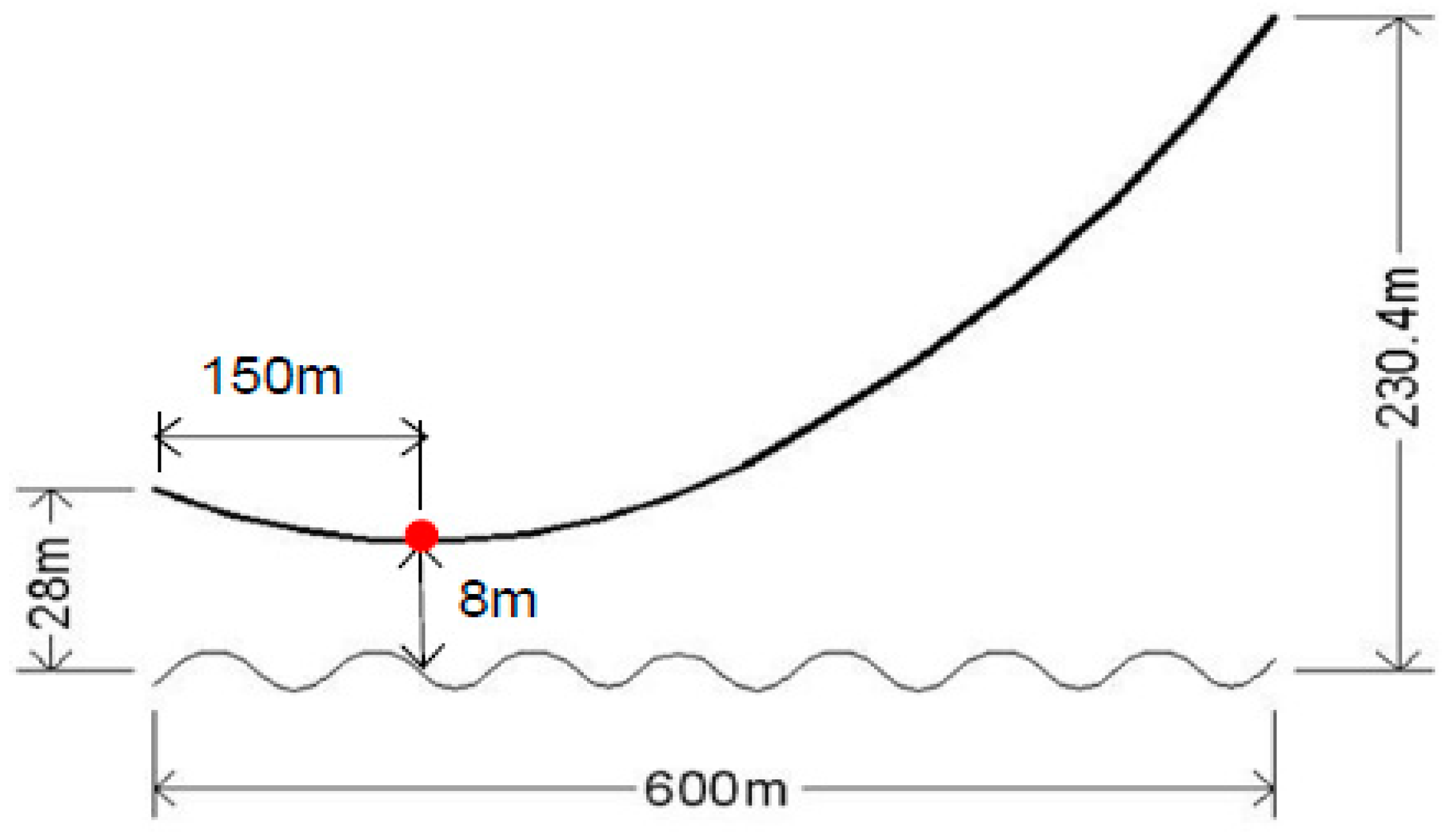
The method presented here makes use of the inverse numerical Laplace transform [17,18] to convert the computed frequency domain solution to a time-domain transient response. This method has strong potential for application in fault location and insulation coordination, with particular accuracy benefits for lines with prominent nonuniformities, such as river crossings, hilly terrains, and other substantial sagging conditions, which are commonly encountered in large countries such as China, Canada, India, Russia, and Brazil. For example, very challenging river crossings are found in Brazil for overhead lines constructed to connect the power generation in the Amazon Basin to the main load centers of the country. These river crossings are in the order of 2 km leading to very tall towers and wide line spans [19]. Accurate fault location under these circumstances requires an appropriate consideration of wave propagation along nonuniform lines, which can be achieved with the method described here. Additionally, the proposed method can be expanded to the modeling of other power system nonuniform elements, such as transmission towers [20] and rotating machines [21].

In order to validate the accuracy of the proposed method, the results obtained are compared with those obtained from simulations performed with ATP (Alternative Transients Program) [22]. In the ATP simulations, the J. Marti line model [23] was used, and the transmission line was subdivided into several line segments to allow the connection of measuring probes at internal points of the line, as well the inclusion of nonuniformities.

The computation of transient profiles along nonuniform transmission lines including nonlinear and time-varying conditions has not been previously reported, providing an original contribution to the current state of the art of the topic.

2. Nonuniform Transmission Line Model for the Transients Profiles Computation

This section describes the transmission line model used to compute the transient profiles as well as the technique used to include time-varying and nonlinear elements. Additionally, a brief explanation for the implementation of the INLT algorithm is presented.

2.1. Nonuniform Transmission Line Model

This work introduces the nonuniformities along transmission lines by means of the technique of cascade connection of chain matrices, as it has been previously shown to be an effective technique for the simulation of electromagnetic transients when nonuniform transmission lines are considered [11,24].

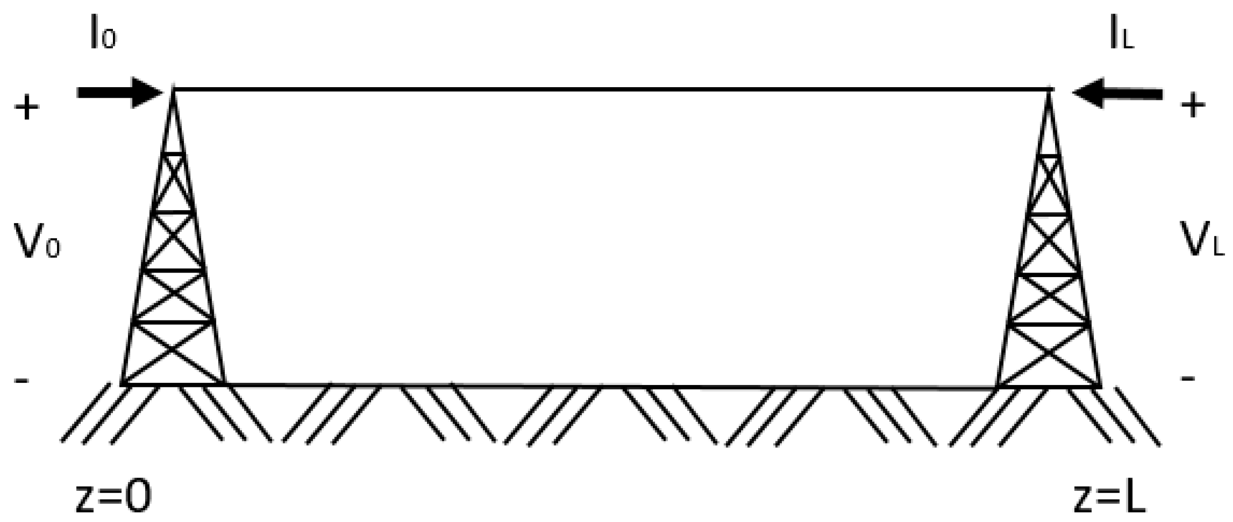
Initially, the uniform transmission line of Figure 1 is considered. This line can be represented by a two-port model known as transfer or ABCD matrix model:

$$\left[\begin{array}{c}{\mathit{V}}_L\left(s\right)\\ {\mathit{I}}_L\left(s\right)\end{array}\right]=\left[\begin{array}{cc}\mathit{A}& \mathit{B}\\ \mathit{C}& \mathit{D}\end{array}\right]\left[\begin{array}{c}{\mathit{V}}_0\left(s\right)\\ {\mathit{I}}_0\left(s\right)\end{array}\right]$$

(1)

where

$$\begin{gathered} \mathit{A}=\cosh \left(\mathbf{\gamma }L\right) \\ \mathit{B}=-{\mathit{Z}}_0\sinh \left(\mathbf{\gamma }L\right) \\ \mathit{C}={\mathit{Y}}_0\sinh \left(\mathbf{\gamma }L\right) \\ \mathit{D}=-\cosh \left(\mathbf{\gamma }L\right) \\ \gamma =\sqrt{\mathit{Z}\mathit{Y}} \end{gathered}$$

(2)

In Equation (2) Z₀, Y₀, Z, Y, and L are the line’s characteristic impedance, characteristic admittance, series impedance, shunt admittance and length, respectively. Additionally, the Laplace variable is defined as $s=c+j\omega$, where $\omega$ is given by $2\pi f$.

By changing the direction of I_L in Figure 1, Equation (1) is modified in the following manner:

$$\left[\begin{array}{c}{\mathit{V}}_L\left(s\right)\\ {\mathit{I}}_L\left(s\right)\end{array}\right]=\left[\begin{array}{cc}\mathit{A}& \mathit{B}\\ -\mathit{C}& -\mathit{D}\end{array}\right]\left[\begin{array}{c}{\mathit{V}}_0\left(s\right)\\ {\mathit{I}}_0\left(s\right)\end{array}\right]$$

(3)

or in a compact form:

$$\left[\begin{array}{c}{\mathit{V}}_L\left(s\right)\\ {\mathit{I}}_L\left(s\right)\end{array}\right]=\Phi \left[\begin{array}{c}{\mathit{V}}_0\left(s\right)\\ {\mathit{I}}_0\left(s\right)\end{array}\right]$$

(4)

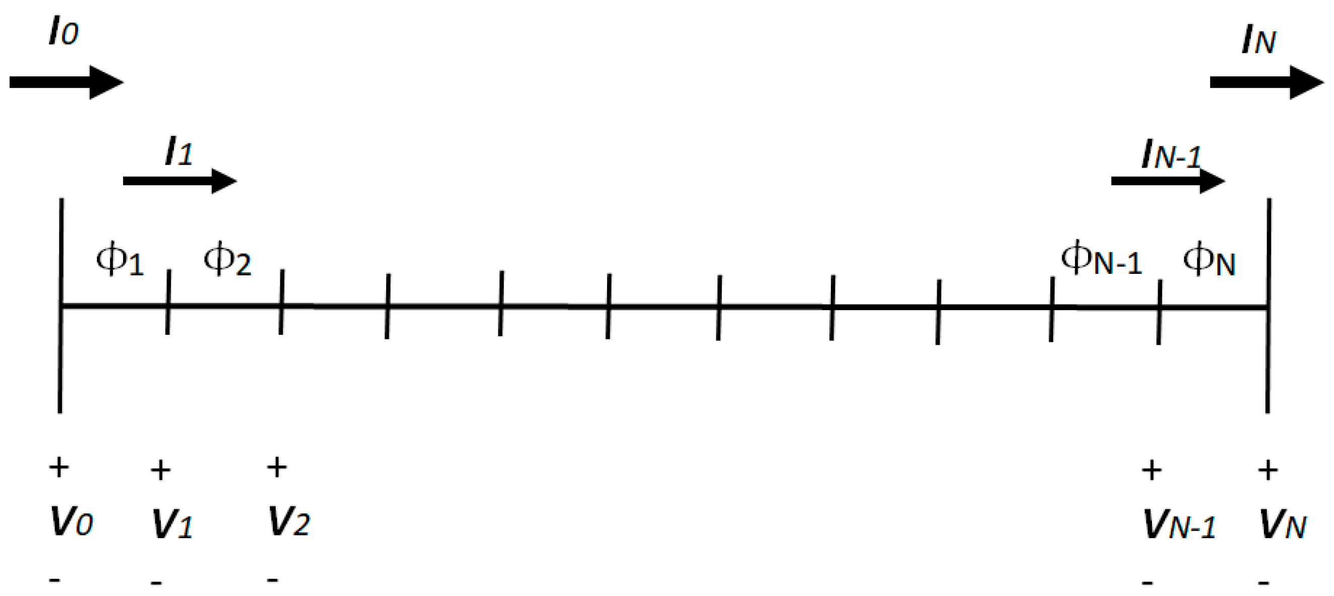
Matrix Φ in Equation (4) is the chain matrix of the transmission line. Due to the fact that the currents at both ends of the line have the same direction, multiple transmission lines can be cascade-connected by using their corresponding chain matrices, as it can be seen in Figure 2.

Figure 2 can also be interpreted as one transmission line subdivided into several smaller line segments, where each segment is represented by a unique chain matrix with its own independent electrical properties. Using this approach, it is possible to build a transmission line model that includes nonuniformities. With this consideration in mind, it can be deduced from Figure 2 that the voltage and current at the beginning of each line segment and the chain matrix of the same segment can be used to compute the voltage and current of the next segment:

$$\begin{gathered} \left[\begin{array}{c}{\mathit{V}}_1\left(s\right)\\ {\mathit{I}}_1\left(s\right)\end{array}\right]={\Phi }_1\left[\begin{array}{c}{\mathit{V}}_0\left(s\right)\\ {\mathit{I}}_0\left(s\right)\end{array}\right] \\ \left[\begin{array}{c}{\mathit{V}}_2\left(s\right)\\ {\mathit{I}}_2\left(s\right)\end{array}\right]={\Phi }_2\left[\begin{array}{c}{\mathit{V}}_1\left(s\right)\\ {\mathit{I}}_1\left(s\right)\end{array}\right]= {\Phi }_2{\Phi }_1\left[\begin{array}{c}{\mathit{V}}_0\left(s\right)\\ {\mathit{I}}_0\left(s\right)\end{array}\right] \end{gathered}$$

(5)

or in a general way:

$$\left[\begin{array}{c}{\mathit{V}}_N\left(s\right)\\ {\mathit{I}}_N\left(s\right)\end{array}\right]={\Phi }_N{\Phi }_{N-1}\dots {\Phi }_3{\Phi }_2{\Phi }_1\left[\begin{array}{c}{\mathit{V}}_0\left(s\right)\\ {\mathit{I}}_0\left(s\right)\end{array}\right]$$

(6)

Equation (6) can be used to compute the voltage and current profiles along a nonuniform transmission line. The transient profiles are computed in a sequential manner, obtaining the voltage and current at the end of the first line segment from the chain matrix and from the voltages and currents at the beginning of the same segment; this process is repeated until the voltage and current along the whole line have been computed. It can also be observed in Equation (6) that V₀ and I₀ are required as initial values of the algorithm; in order to compute such values, a two-port admittance representation of the complete transmission line from the chain matrix Φ_FL is defined as:

$${\Phi }_{FL}={\Phi }_N{\Phi }_{N-1}\dots {\Phi }_3{\Phi }_2{\Phi }_1=\left[\begin{array}{cc}{\Phi }_{FL11}& {\Phi }_{FL12}\\ {\Phi }_{FL21}& {\Phi }_{FL22}\end{array}\right]$$

(7)

$$\left[\begin{array}{c}{\mathit{I}}_0\left(s\right)\\ {\mathit{I}}_L\left(s\right)\end{array}\right]=\left[\begin{array}{cc}{\mathit{Y}}_{ss}& -{\mathit{Y}}_{sr}\\ -{\mathit{Y}}_{rs}& {\mathit{Y}}_{rr}\end{array}\right]\left[\begin{array}{c}{\mathit{V}}_0\left(s\right)\\ {\mathit{V}}_L\left(s\right)\end{array}\right]$$

(8)

where

$$\begin{gathered} {\mathit{Y}}_{ss}=-{\Phi }_{FL12}^{-1}{\Phi }_{FL11} \\ {\mathit{Y}}_{sr}=-{\Phi }_{FL12}^{-1} \\ {\mathit{Y}}_{rs}={\Phi }_{FL21}-{\Phi }_{FL22}{\Phi }_{FL12}^{-1}{\Phi }_{FL11} \\ {\mathit{Y}}_{rr}=-{\Phi }_{FL22}{\Phi }_{FL12}^{-1} \end{gathered}$$

(9)

V₀(s) is obtained by solving (8) for the voltages vector. I₀(s) is computed as follows:

$${\mathit{I}}_0\left(s\right)={\mathit{Y}}_{ss}{\mathit{V}}_0\left(s\right)-{\mathit{Y}}_{rr}{\mathit{V}}_L\left(s\right)$$

(10)

2.2. Modeling of Time-Varying Elements

It can be difficult to include time-varying conditions, such as switching maneuvers, when methods defined in the frequency domain are used to simulate electromagnetic transients. However, the principle of superposition has demonstrated to be an efficient method to include such conditions in the frequency domain [25], as explained below.

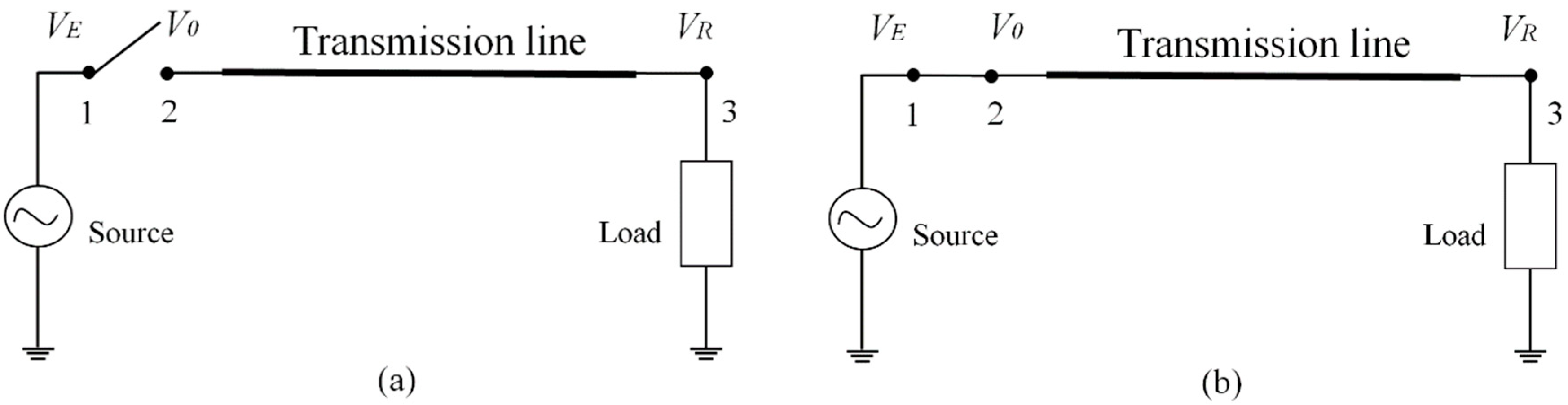
The closing of a switch can be computed using the circuits presented in Figure 3, which represent the state of the circuit before and after the closing maneuver. V_E, V_S, and V_R are the voltage at the source side, at the line’s sending node, and at the line’s receiving node, respectively. The nodal voltage vector V_NL(s) is formed by the three subvectors in Figure 3 as shown below:

$${\mathit{V}}_{NL}\left(s\right)={\left[\begin{array}{ccc}{\mathit{V}}_E\left(s\right)& {\mathit{V}}_0\left(s\right)& {\mathit{V}}_L\left(s\right)\end{array}\right]}^T$$

(11)

and can be obtained from the following expression [11]:

$${\mathit{V}}_{NL}\left(s\right)=\mathit{Y}\mathit{b}\mathit{u}{\mathit{s}}_0^{-1}{\mathit{I}}_{N0}+\mathit{Y}\mathit{b}\mathit{u}{\mathit{s}}_1^{-1}{\mathit{I}}_{N1}$$

(12)

In Equation (12), Ybus₀ is the nodal admittance matrix before the switch closing (Figure 3a), Ybus₁ is the admittance matrix modified by the closing operation (Figure 3b), I_N0 contains the initially injected currents, and I_N1 is the injection current vector due to the switch operation. An example of the construction of the nodal admittance matrices Ybus₀ and Ybus₁ for the transmission line in Figure 3 is presented below:

$$\mathit{Y}\mathit{b}\mathit{u}{\mathit{s}}_{0,1}\left[\begin{array}{ccc}{Y}_{11}& -Y_{12}& -Y_{13}\\ -Y_{21}& Y_{22}& -Y_{23}\\ -Y_{31}& -Y_{32}& Y_{33}\end{array}\right]$$

(13)

If Ybus₀ (Figure 3a) is to be built using (13), the elements $Y_{11}$, $Y_{12}$, $Y_{21}$, and $Y_{22}$ would assume the following values: $Y_{12}=Y_{21}=Y_{switcho}$, where $Y_{switcho}$ is the open switch’s admittance between its poles, ideally $Y_{switcho}=0$. $Y_{11}=Y_s+Y_{swtcho}$, with $Y_s$ being the admittance connected at the sending node, and $Y_{22}=Y_{LL}+Y_{switcho}$ where $Y_{LL}$ represents the self-admittance of the transmission line. The matrix Ybus₁ (Figure 3b) can be built in a similar way, but replacing $Y_{switcho}$ by $Y_{switchc}$, that is, the admittance of the switch when closed.

The procedure presented above can be extended to any number of changes in the circuit topology using the following expression:

$${\mathit{V}}_{NL}\left(s\right)=\mathit{Y}\mathit{b}\mathit{u}{\mathit{s}}_0^{-1}{\mathit{I}}_{N0}+{\displaystyle \sum }_{i=1}^m\mathit{Y}\mathit{b}\mathit{u}{\mathit{s}}_i^{-1}{\mathit{I}}_{Ni}$$

(14)

where Ybus_i and I_Ni are the modified admittance matrix and the injection current vector corresponding to the n-th switch operation, respectively. A comprehensive explanation of this procedure can be found in [11].

V₀(s) in (11) is the voltage at the sending node of the line needed in (6) to compute the transient voltage and current profiles. Meanwhile, the current at the beginning of the line is computed with (10) using V₀(s) and V_L(s) from (11).

2.3. Inclusion of Nonlinear Elements

It has been demonstrated that the principle of superposition can be used to overcome the difficulties of the inclusion of nonlinear components in the frequency domain [25]. This is achieved by means of a sequence of switching operations.

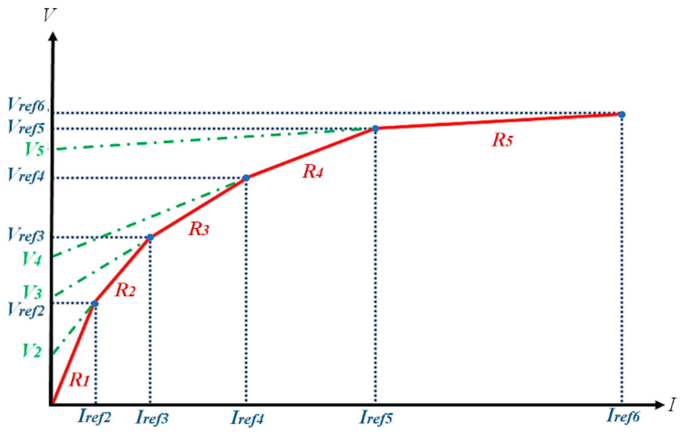
In order to include a nonlinear element in a simulation performed using a method based in the frequency domain, first, its nonlinear characteristic curve must be approximated by a piece-wise curve, as illustrated in Figure 4.

The element R_n of the n-th linear element from Figure 4 and the voltage V_n are computed as follows:

$$R_n=\frac{V_{refn+1}-V_{refn}}{I_{refn+1}-I_{refn}}$$

(15)

$$V_n=\left(-R_{n+1}{I}_{refn}\right)+V_{refn+1}$$

(16)

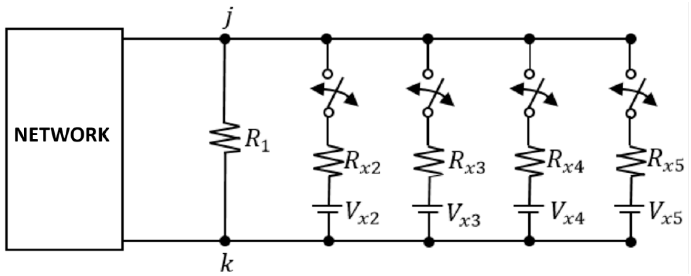
By approximating the v-i characteristic of a nonlinear element as shown above, such an element can be represented as a network of N parallel-connected branches, as shown in Figure 5.

In the circuit presented in Figure 5, the switch in the n-th branch operates according to the reference voltage; it closes when the voltage across nodes j and k goes above V_refn and it opens when the voltage drops below V_refn. It is important to mention that the switches must operate in a successive manner, meaning that a switch can only close when the one in the preceding branch is closed, and a switch can only open when the one in the following branch is open.

When the switch connected to the n-th branch is closed, the equivalent Thevenin resistance of the circuit in Figure 5 must be equal to the value of $R_n$, that is, the slope of the n-th linear segment in the approximation of Figure 4:

$$R_n=\frac{R_{n-1}{R}_{xn}}{R_{n-1}+R_{xn}}$$

(17)

Finally, by solving (17) for $R_{xn}$, the value of such resistance can be computed:

$$R_{x_n}=\frac{R_{n-1}{R}_n}{R_{n-1}-R_n}$$

(18)

V_xn is computed as:

$$V_{x_n}=\frac{R_{n-1}{V}_n-V_{n-1}{R}_n}{R_{n-1}-R_n}$$

(19)

With this approach, it is possible to compute the transient profiles along nonuniform transmission lines with nonlinear and/or time-varying elements using (6), calculating the voltage and current at the sending node with (10) and (14), and implementing the nonlinear element model presented in this section.

2.4. Inverse Numerical Laplace Transform

As the last step, the INLT is applied to the computed transient profiles in the frequency domain with (6); this is done in order to transform the results to the time domain. This method has proven to be very accurate for the study of electromagnetic transients [11,24,25]. The implementation of the INLT algorithm is described below in a brief manner; references [17,18] can be consulted for a thorough explanation. Considering a time function $f\left(t\right)$ as a real and causal function, the inverse Laplace transform can be written as:

$$f\left(t\right)=Re\left\{\frac{e^{ct}}{2\pi }\underset{0}{\overset{\infty }{{\displaystyle \int }}}F\left(s\right)e^{j\omega t}d\omega \right\}$$

(20)

In this work, the numerical evaluation of (20) is done considering an odd sampling in the frequency spectrum (using a spacing of $2\Delta \omega$), and normal time steps $\Delta t$ in the time domain. With these considerations in mind, the following definitions for the discrete functions in the time and frequency domain for N equally spaced samples are made:

$$\begin{gathered} f_n=f\left(n\Delta t\right) \\ {F}_m=F\left(c+j\left(2m+1\right)\Delta \omega \right) \end{gathered}$$

(21)

where $n,m=0, 1, 2, \dots , N-1$ and $c$hat reduces the aliasing errors of the algorithm; in this work, $c$ is defined as $c=2\Delta \omega$.

Additionally, it is necessary to establish finite integration limits for the numerical evaluation of (20), that is, the maximum frequency $\mathsf{\Omega }$ and the observation time T. The observation time is computed from:

$$T=\frac{\pi }{\Delta \omega }$$

(22)

and the following relations can be established:

$$\begin{gathered} \Delta t=\frac{T}{N} \\ \Delta \omega =\frac{\mathsf{\Omega }}{2N}=\frac{\pi }{T} \end{gathered}$$

(23)

Finally, by implementing the odd sampling presented in (21) and including a window function ${\sigma }_m$, the Laplace transform in (20) can be numerically approximated by:

$$f_n=Re\left\{C_n\left[{\displaystyle \sum }_{m=0}^{N-1}{F}_m{\sigma }_{m}exp\left(\frac{j2\pi m}{N}\right)\right]\right\}\mathrm{for}n,m=0,1,2,\dots ,N–1$$

(24)

where:

$$C_n=\frac{2\Delta \omega }{\pi }exp\left(cn\Delta t+\frac{j\pi n}{N}\right)$$

(25)

In Equation (24), the term inside the brackets corresponds to the fast Fourier transform algorithm; this allows computing time savings if $N$ is equal to an integer power of two.

3. Test Cases

Three test cases are presented in order to validate the proposed method. The frequency dependence of the line’s electrical parameters was taken into account by means of the application of the complex image method to introduce the earth-return impedance, as well as the complex penetration depth to include the skin effect in the line conductors [26]. The accuracy of the method was validated through comparisons with measurements from simulations performed with ATP, where the frequency-dependent J. Marti line model was discretized in several smaller segments to allow the introduction of nonuniformities and the connection of measuring probes at interior points. The length of the simulated lines in the test cases was kept short in order to reduce the implementation burden in ATP; with the proposed method, the length and discretization of the line did not represent a problem.

3.1. Highly Nonuniform Transmission Line

A highly nonuniform three-phase transmission line was considered. The nonuniformity was included by the sagging of the conductors as shown in Figure 6. The line was excited by an ideal unit step voltage source (1 p.u.) connected at phase A of the sending node, while all of the other nodes were left open.

Figure 7 presents the transient voltage profile along phase A computed with the proposed method; in order to include the nonuniformities along the transmission line, it was subdivided into 80 chain matrices. This figure illustrates the propagation of the traveling waves along the line and how these waves were reflected when they reached the receiving end. It can also be observed in the transient profiles that there were periods where negative voltages appeared at some points along the line, which is not a commonly observed phenomenon when similar simulations with uniform lines are performed. Additionally, a comparison at the middle of the line between the transient voltage waveforms obtained with the proposed method and results from ATP simulations is presented (Figure 8). The simulations performed with ATP required a time step 10 times smaller than the proposed method to achieve similar results.

This example was simulated with the proposed method considering 20 and 40 chain matrices. Figure 9 presents a comparison of voltage measurements at the middle point of the transmission line from simulations considering 20, 40, and 80 chain matrices. From this comparison, it can be observed that the curves from the three simulations, in general, have the same shape (curves for 40 and 80 chain matrices are overlapped). However, the curve corresponding to the simulation performed with 20 chain matrices presents some oscillations in comparison with the other two. As it can be seen with the curves corresponding to 40 and 80 chain matrices, with an increase in the number of chain matrices used in the simulations, the curves become smoother; however, a further increase in the number of chain matrices used is barely noticeable. This indicates that although the method’s accuracy is dependent on the number of chain matrices considered, it does not require a large number of chain matrices to achieve good results.

3.2. Sequential Energization

A 5 km transmission line was used in this case. The nonuniformity was introduced by means of the line’s sag: there was a transmission tower every 500 m, the conductors’ height was maximum at the towers (20 m), and the height was minimum at the midspan between towers (15 m). The consideration for the height’s variation as well as the horizontal separation between conductors was the same as in the previous example. The line was connected to an AC voltage source (1 p.u.) at the sending node through a three-phase switch. The switch’s poles operated in a sequential manner with closing times of 3, 6, and 9 ms in an ABC sequence. The line’s receiving node was left open.

The transient voltage profiles of phases A and B are presented in Figure 10 and Figure 11, respectively. The comparison with ATP simulations is shown in Figure 12.

3.3. Surge Arrester Operation

This example presents the operation of surge arresters during a direct lightning strike; due to their v-i characteristic, the arresters were modeled as nonlinear elements as described in Section 2.3. The same line configuration presented in Section 3.1 was considered. The line was excited by a direct lightning strike (1.2/50 µs), the impact point was at the phase A of the sending node, and the line was impedance-matched at both ends in order to avoid reflections. The injected current to the line was approximated by a double exponential current source defined as:

$$i\left(t\right)=I_0\left(e^{-\frac{t}{{\tau }_1}}-e^{-\frac{t}{{\tau }_2}}\right)$$

(26)

where τ₁ = 68.199 µs, τ₂ = 0.405 µs, and I₀ = 10.37 kA.

Surge arresters were connected to the three phases at the receiving node. The nonlinear characteristic of the arresters was simulated by means of a five-segment piecewise-linear approximation.

Table 1. Nonlinear v-i characteristic of the arresters [27].

Vref (kV)	Iref (kA)
0	0
484	0.1760
616	0.3226
748	0.7626
836	1.6426
880	12.6426

presents the v-i coordinates of this representation.

First, a simulation was performed without surge arresters connected to the line. Figure 13 presents the transient voltage profile along phase A computed in this simulation. On the other hand, Figure 14 shows the voltage profile along phase A when the arresters were connected at the receiving node of the line. By comparing Figure 13 and Figure 14, the influence that the surge arresters’ operation had on the magnitude of the voltages along the line is easily observed. The voltage along the line in Figure 14 was considerably lower in comparison with the transient profile in Figure 13. Additionally, a comparison is presented with results obtained from ATP simulations (Figure 15). In a similar way to the example in Section 3.1, the time step required by ATP was 10 times smaller than the proposed method in order to obtain similar results.

4. Discussion

Transient simulation of nonuniform transmission lines using traditional software (such as ATP in this paper) is a challenging task. This difficulty is due to the fact that the nonuniformities are typically approximated by cascade-connecting several small line segments. Such approximation requires the use of a very small time step in the simulation (at least five times smaller than the traveling time of the line segments [6]), which may translate into excessive simulation times and the saturation of the software’s available memory, as was the case in this work. Additionally, the connection of several line segments can introduce errors in the simulation results [2].

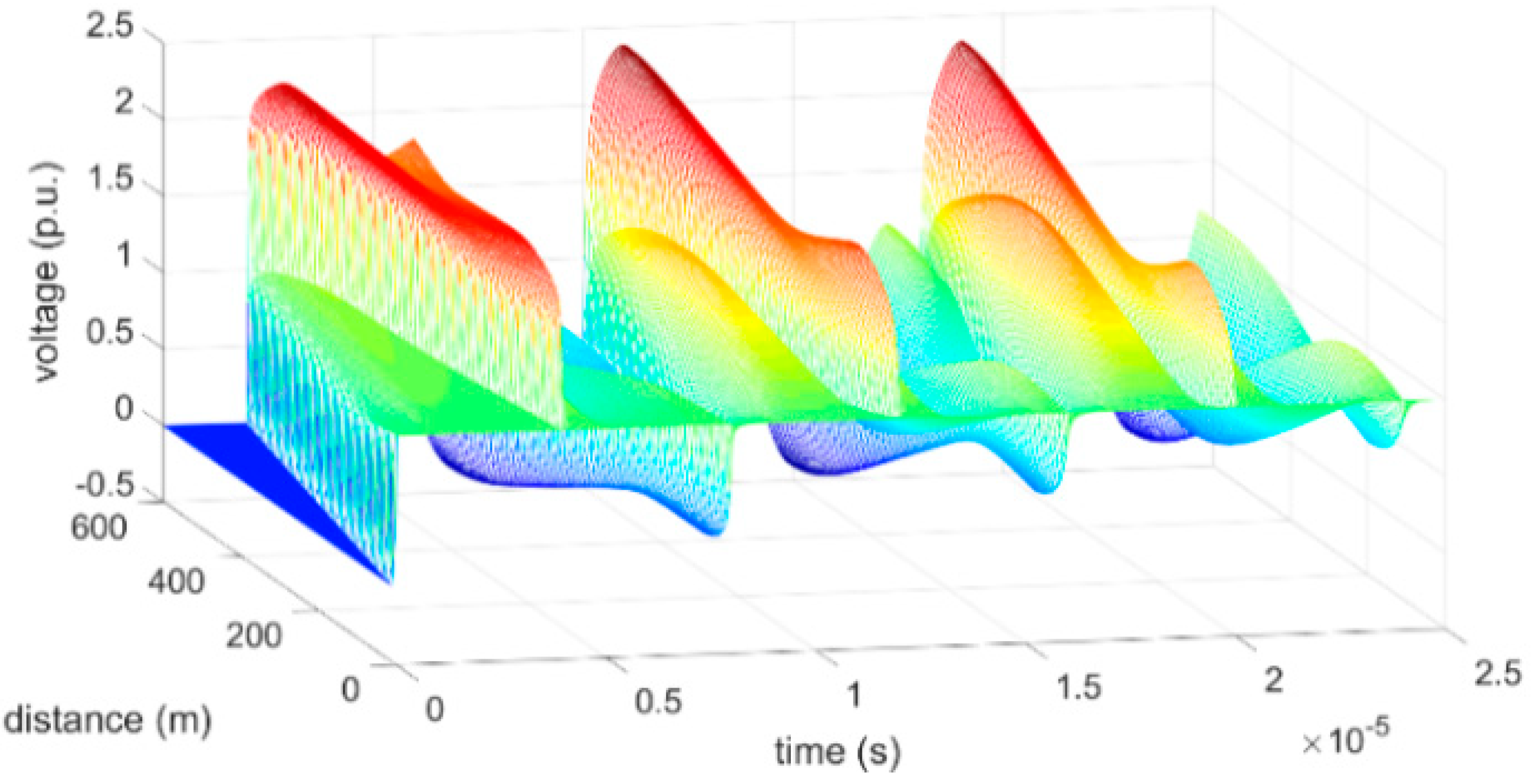
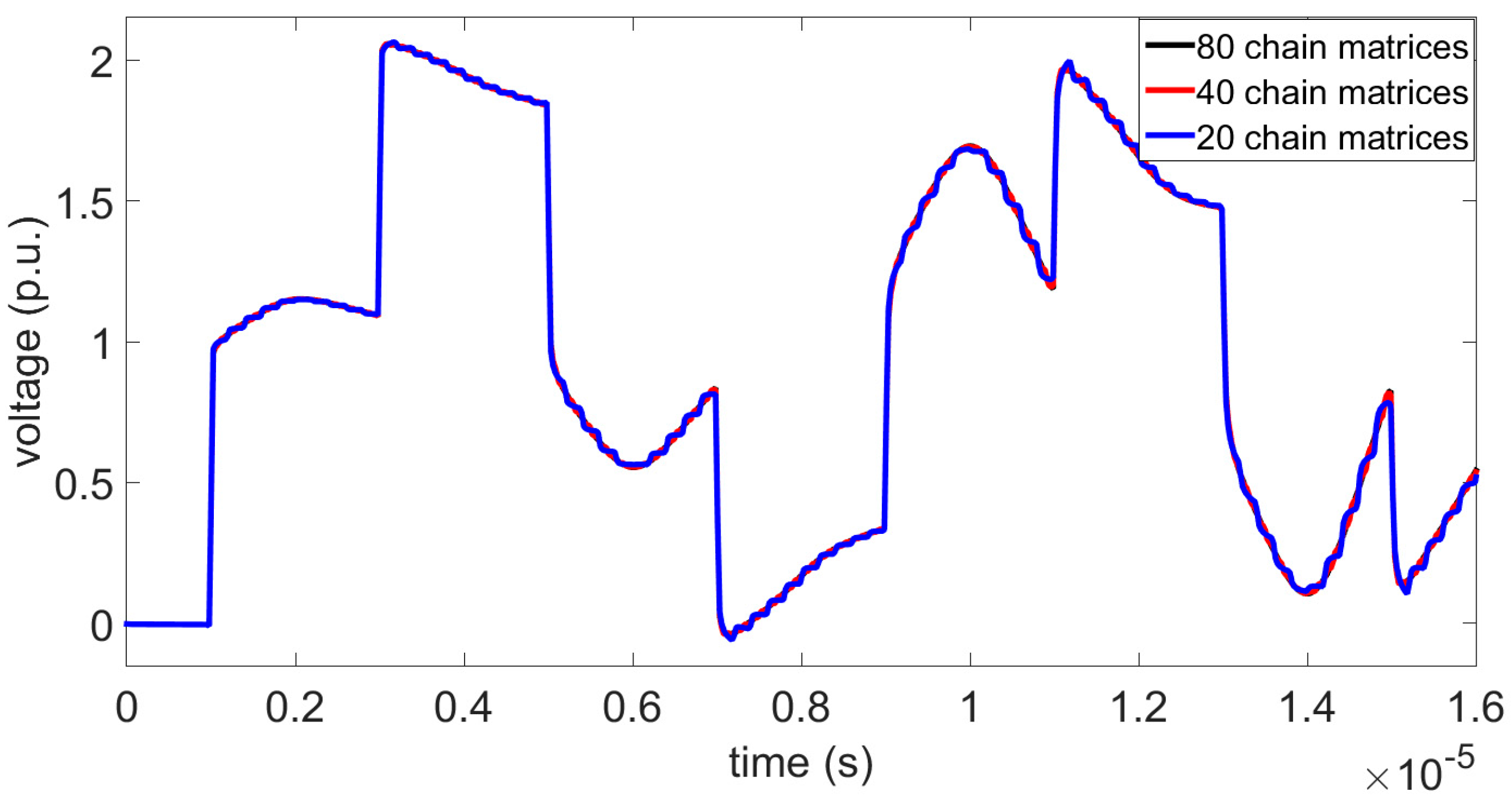
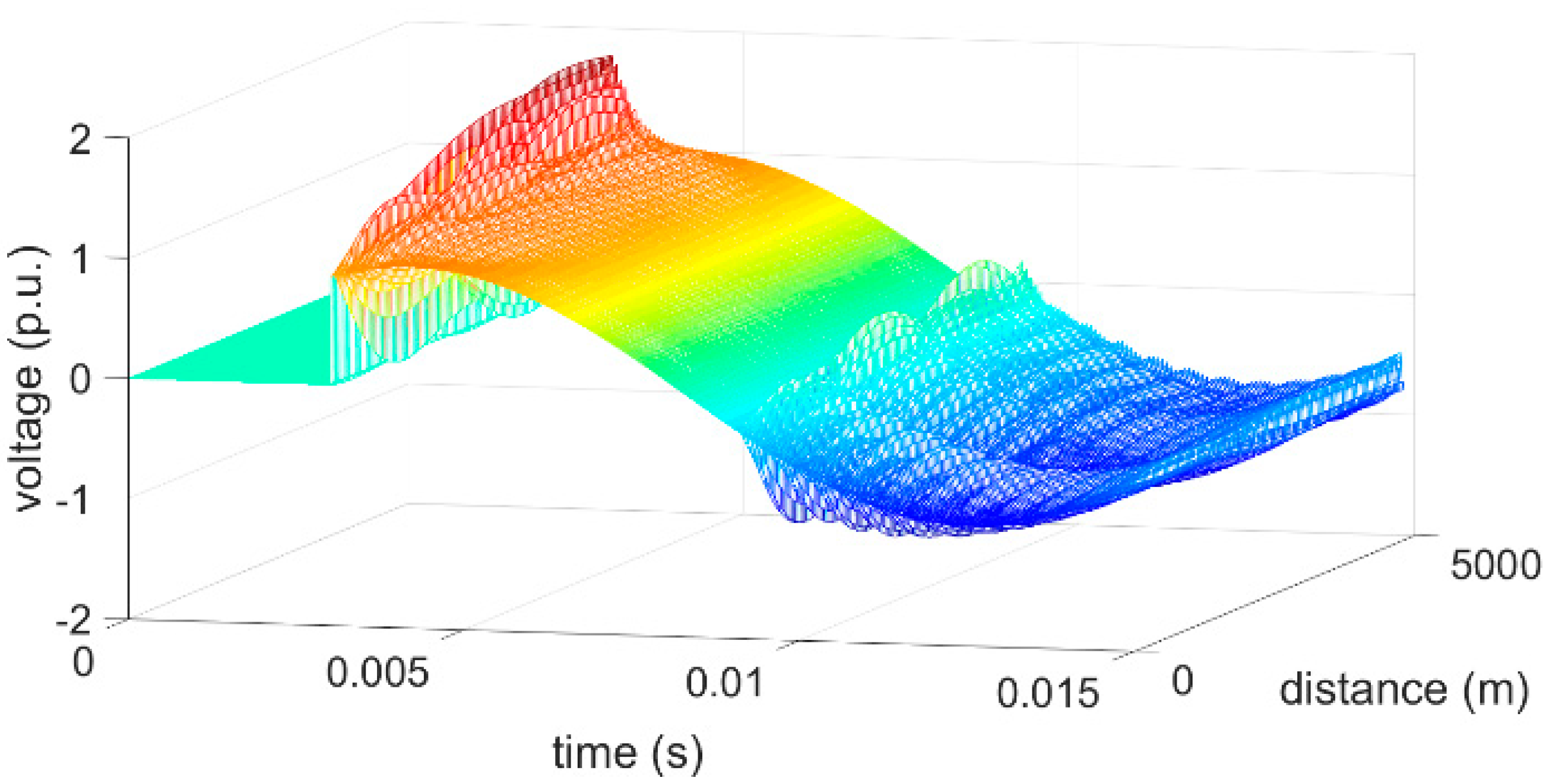
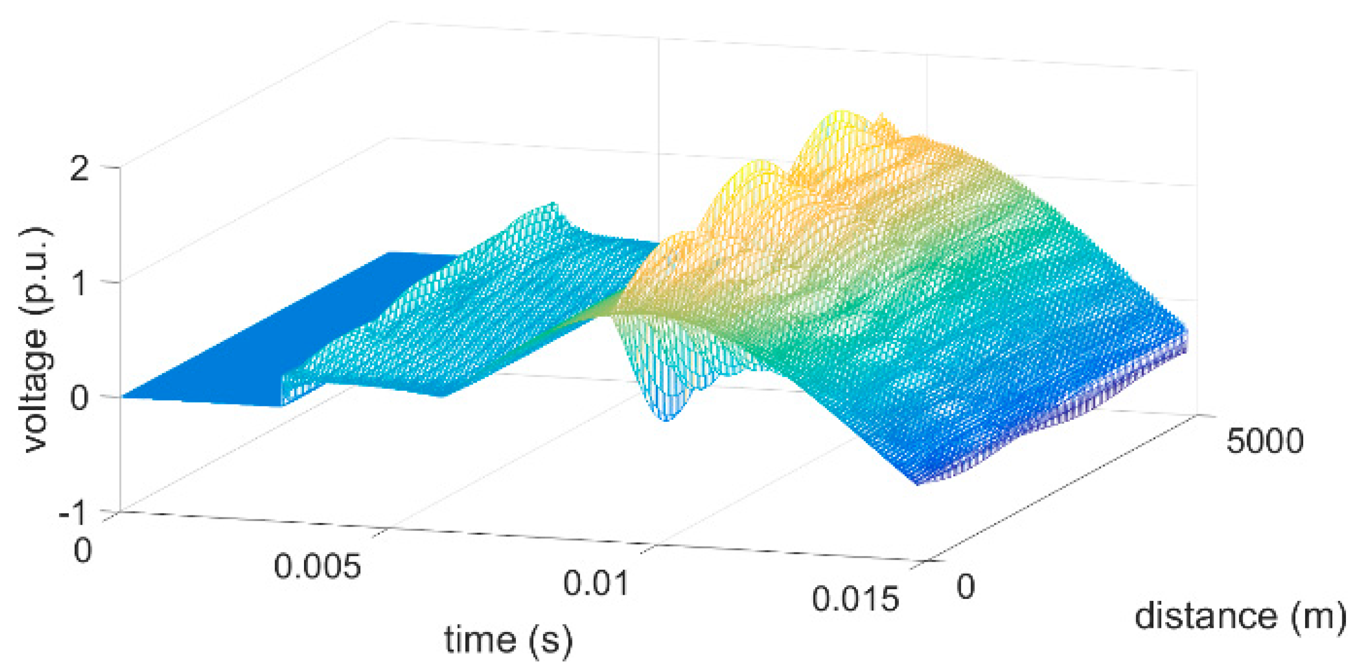
In contrast, the proposed method is able to accurately compute transient profiles along nonuniform transmission lines with substantially larger time steps in comparison to ATP, resulting in a better memory usage as expected from the findings reported in [16] with regards to the use of the INLT algorithm. As it can be observed in Figure 7, Figure 10, Figure 11 and Figure 14, the main advantage of the proposed method is the fact that it allows visualizing the voltage and current transient behavior along the line and not only at its ends, which can be advantageous when designing lines with a high level of nonuniformities and cannot be easily done using traditional simulation software.

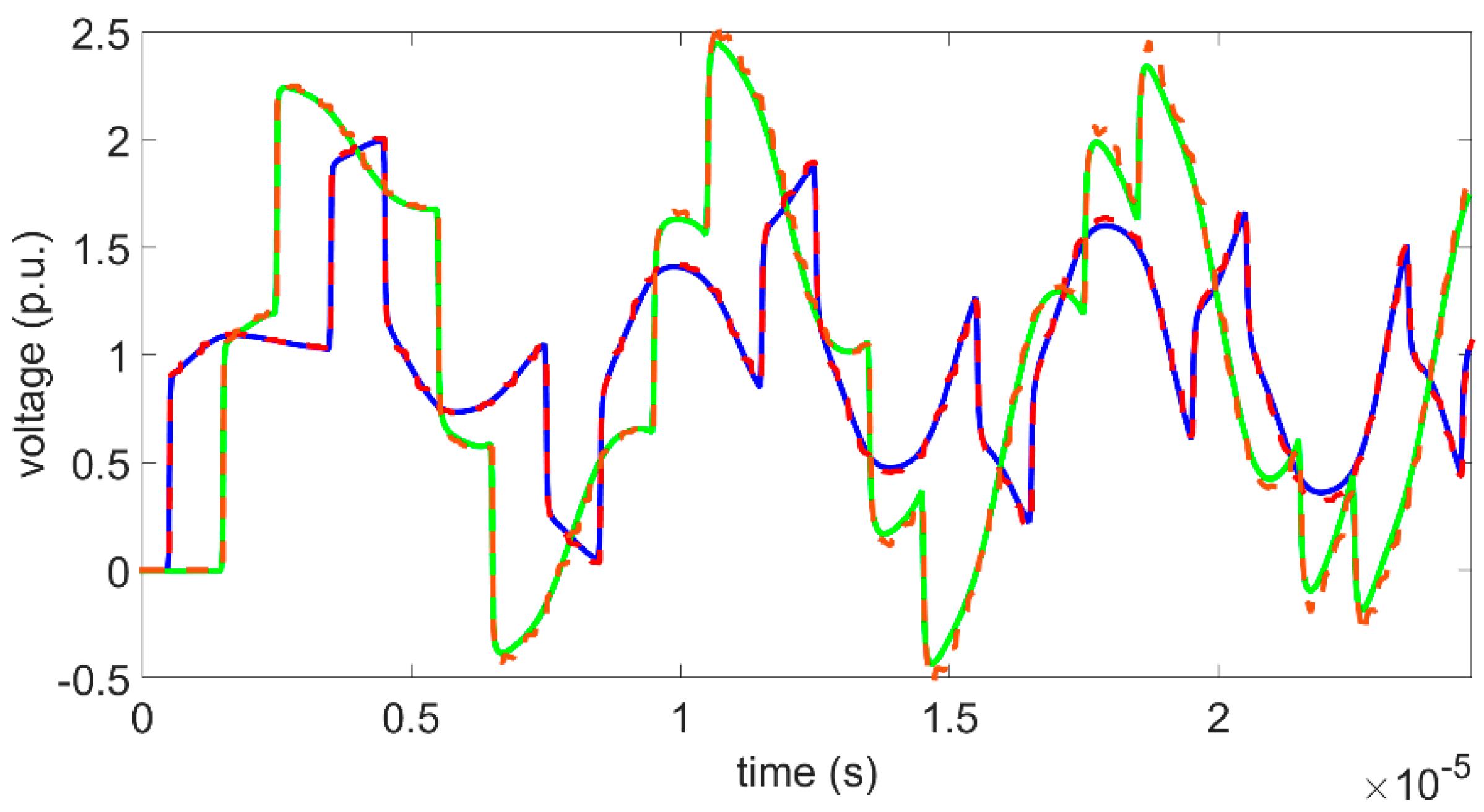
The precision of the proposed method was validated by comparisons with the results obtained with ATP simulations. In general, there was a very good level of agreement between the results from both methods, as it can be seen by the mean relative difference presented in

Table 2. Mean relative difference of transient voltage in example 3.1.

Measuring Point	Mean Relative Difference (%)
	Phase A	Phase B	Phase C
150 m	0.0708	0.1837	0.2893
450 m	0.3839	0.3351	0.6832

,

Table 3. Mean relative difference of transient voltage in example 3.2.

Measuring Point	Mean Relative Difference (%)
	Phase A	Phase B	Phase C
2.5 km	0.3889	0.9861	1.2761

and

Table 4. Mean relative difference of transient voltage in example 3.3.

Measuring Point	Mean Relative Difference (%)
	Phase A	Phase B	Phase C
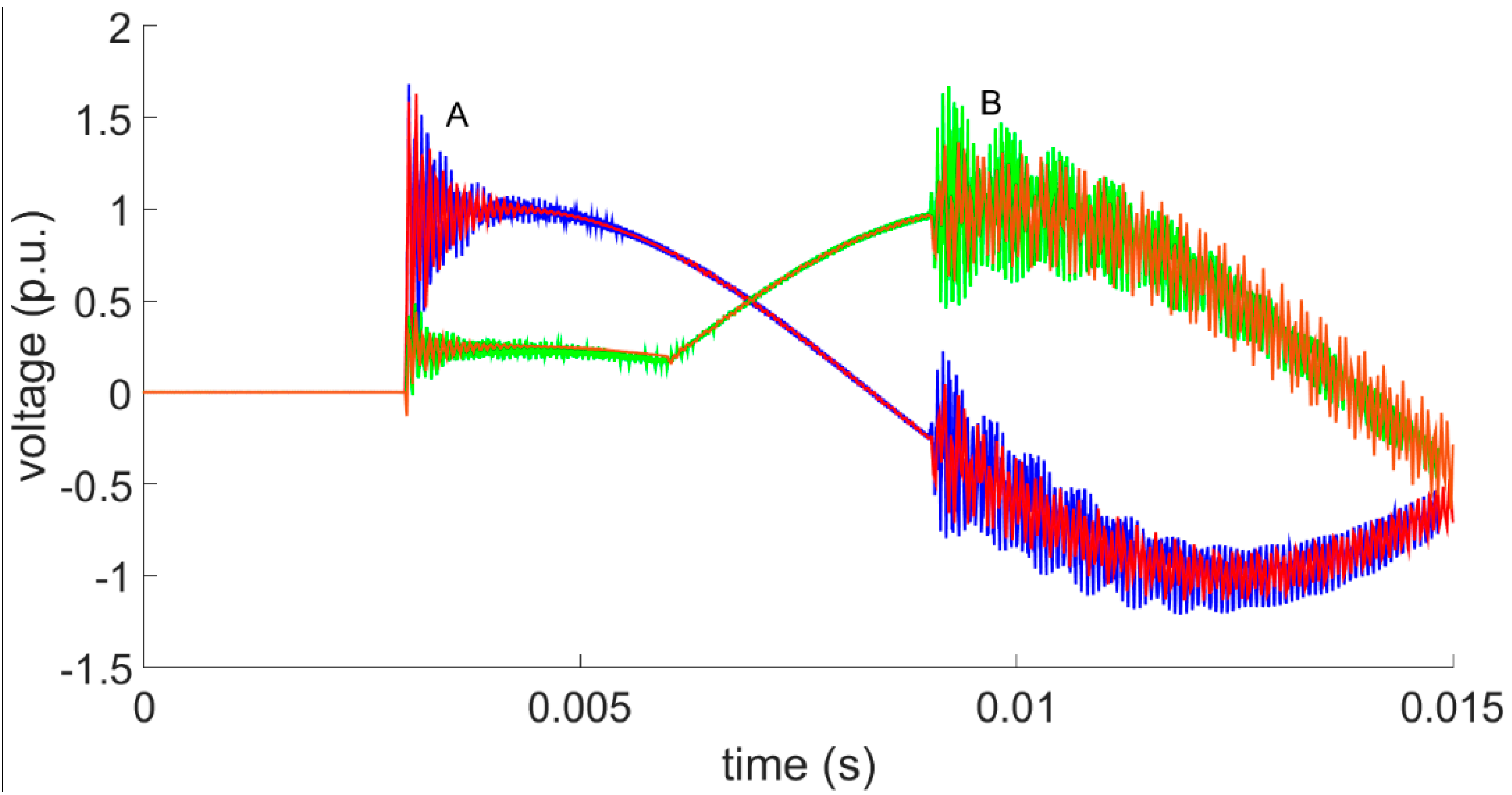
300 m	0.0374	0.7738	1.9183

. There is a slight difference in the comparison of results presented in Figure 12 corresponding to the simulation of sequential pole closure. This is attributed to the previously mentioned ATP limitations and the difference in the time step used in each method, which can result in deviations in the operation time of the switch model, leading to the observed variations.

5. Conclusions

This paper describes a frequency domain method to compute transient voltage and current profiles along nonuniform multiconductor transmission lines, where the nonuniformities along the line are introduced in the model by means of the cascaded connection of chain matrices. The method can incorporate nonlinear and time-dependent elements by using the superposition principle. The profiles obtained provide useful information to locate possible overvoltages at interior points along the transmission line, in contrast to traditional methods that only provide information at the line’s ends. This information can be used as a helpful instrument in the insulation coordination design of transmission lines, as well as an educational tool in electrical engineering courses.

The results computed with the described method were compared with time-domain simulations using the well-known software ATP. In all of the comparisons, a high level of agreement was observed, demonstrating that the proposed method has a high level of accuracy.

It is worth mentioning that, although the results from both methods were very similar, the ATP simulations required substantially more time samples (10 to 50 times more samples) to achieve such results, which can result in a large computational burden. Additionally, in order to obtain measurements at interior points of the transmission line and to include nonuniformities along the transmission line in the ATP simulations, it is necessary to subdivide the line into many line segments, which can be a time-consuming process and can lead to error accumulation. Because of these issues, the proposed frequency domain method is a superior alternative to analyze the transient behavior of a transmission line when the voltage at interior points of the line is of interest.

The relevance of the proposed method lies in its strong potential for application in the accurate fault location and insulation coordination of transmission systems with prominent nonuniformities, which are commonly encountered in many power systems around the world.

References

1. Martínez-Velasco, J.A. Parameter determination for electromagnetic transient analysis in power systems. In Power System Transients: Parameter Determination, 1st ed.; CRC Press: Boca Raton, FL, USA, 2010; pp. 1–16. [Google Scholar]
2. Marti, L.; Dommel, H.W. Calculation of voltage profiles along transmission lines. IEEE Trans. Power Deliv. 1997, 12, 993–998. [Google Scholar] [CrossRef]
3. Pinto, A.J.G.; Costa, E.C.M.; Kurokawa, S.; Monteiro, J.H.A.; de Franco, J.L.; Pissolato, J. Analysis of the electrical characteristics and surge protection of EHV transmission lines supported by tall towers. Int. J. Electr. Power Energy Syst. 2014, 57, 358–365. [Google Scholar] [CrossRef]
4. Pinto, A.J.G.; Costa, E.C.M.; Kurokawa, S.; Pissolato, J. Analysis of the electrical characteristics of an alternative solution for the Brazilian-Amazon transmission system. Electr. Power Comp. Syst. 2011, 39, 1424–1436. [Google Scholar] [CrossRef]
5. Martínez, D.; Moreno, P.; Loo-Yau, R. A new model for non-uniform transmission lines. In Proceedings of the 12th International Conference on Electrical Engineering, Computing Science and Automatic Control (CCE), Mexico City, Mexico, 28–30 October 2015. [Google Scholar]
6. Lima, A.C.S.; Moura, R.A.R.; Gustavsen, B.; Schroeder, M.A.O. Modelling of non-uniform lines using rational approximation and mode revealing transformation. IET Gener. Transm. Distrib. 2017, 11, 2050–2055. [Google Scholar] [CrossRef]
7. Saied, M.M.; Al-Fuhaid, A.S.; El-Shandwily, M.E. S-domain analysis of electromagnetic transients on non-uniform lines. IEEE Trans. Power Deliv. 1990, 5, 2072–2081. [Google Scholar] [CrossRef]
8. Oufi, E.A.; Al-Fuhaid, A.S.; Saied, M.M. Transient analysis of loss-less single phase nonuniform transmission lines. IEEE Trans. Power Deliv. 1994, 9, 1694–1700. [Google Scholar] [CrossRef]
9. Correia de Barros, M.T.; Almeida, M.E. Computation of electromagnetic transients on nonuniform transmission lines. IEEE Trans. Power Deliv. 1996, 11, 1082–1087. [Google Scholar] [CrossRef]
10. Semlyen, A. Some frequency domain aspects of wave propagation on nonuniform lines. IEEE Trans. Power Deliv. 2003, 18, 315–322. [Google Scholar] [CrossRef]
11. Gómez, P.; Escamilla, J.C. Frequency domain modeling of nonuniform multiconductor lines excited by indirect lightning. Int. J. Electr. Power Energy Syst. 2013, 45, 420–426. [Google Scholar] [CrossRef]
12. Nuricumbo-Guillén, R.; Espino-Cortés, F.P.; Gómez, P.; Tejada-Martínez, C. Computation of transient profiles along non-uniform trasmission lines using the numerical Laplace transform. In Proceedings of the IEEE International Conference on High Voltage Engineering and Applications, Athens, Greece, 10–13 September 2018. [Google Scholar]
13. Nuricumbo-Guillén, R.; Gómez, P.; Espino-Cortés, F.P.; Uribe, F.A. Accurate computation of transient profiles along multiconductor transmission lines by means of the numerical Laplace transform. IEEE Trans. Power Deliv. 2014, 29, 2385–2395. [Google Scholar] [CrossRef]
14. Gómez, P.; Vergara, L.; Nuricumbo-Guillén, R.; Espino-Cortés, F.P. Two dimensional definition of the numerical Laplace transform for fast computation of transient profiles along power transmission lines. IEEE Trans. Power Deliv. 2016, 31, 412–414. [Google Scholar] [CrossRef]
15. Nuricumbo-Guillén, R.; Vergara, L.; Gómez, P.; Espino-Cortés, F.P. Laplace-based computation of transient profiles along transmission lines including time-varying and non-linear elements. Int. J. Electr. Power Energy Syst. 2019, 106, 138–145. [Google Scholar] [CrossRef]
16. Brancik, L. Time and Laplace-domain methods for MTL transient sensitivity analysis. Int. J. Comput. Math. Electr. Electron. Eng. 2011, 30, 1205–1223. [Google Scholar] [CrossRef]
17. Gómez, P.; Uribe, F.A. The numerical Laplace transform: An accurate tool for analyzing electromagnetic transients on power system devices. Int. J. Electr. Power Energy Syst. 2009, 31, 116–123. [Google Scholar] [CrossRef]
18. Moreno, P.; Ramírez, A. Implementation of the numerical Laplace transform: A review. IEEE Trans. Power Deliv. 2008, 23, 2599–2609. [Google Scholar] [CrossRef]
19. Souza, L.; Lima, A.C.S.; Carneiro, S., Jr. Modeling Overhead Transmission Line with Large Asymmetrical Spans. In Proceedings of the 2011 International Conference on Power Systems Transients, Delft, The Netherlands, 14–17 June 2011. [Google Scholar]
20. Guo, X.; Fu, Y.; Yu, J.; Xu, Z. A non-uniform transmission line model of the ±1100 kV UHV tower. Energies 2019, 12, 445. [Google Scholar] [CrossRef]
21. Hussain, M.K.; Gómez, P. Optimal filter tuning to minimize the transient overvoltages on machine windings fed by PWM inverters. In Proceedings of the 2017 North American Power Symposium (NAPS), Morgantown, VA, USA, 17–19 September 2017. [Google Scholar]
22. Dommel, H.W. Electromagnetic Transient Program Theory Book; Bonneville Power Administration: Portland, OR, USA, 1986. [Google Scholar]
23. Marti, J. Accurate modelling of frequency-dependent transmission lines in electromagnetic transient simulations. IEEE Trans Power App. Syst. 1982, PAS-101, 147–157. [Google Scholar] [CrossRef]
24. Gómez, P.; Moreno, P.; Naredo, J.L. Frequency domain transient analysis of nonuniform lines with incident field excitation. IEEE Trans. Power Deliv. 2005, 20, 2273–2280. [Google Scholar] [CrossRef]
25. Moreno, P.; Gómez, P.; Naredo, J.L.; Guardado, J.L. Frequency domain transient analysis of electrical networks including non-linear conditions. Int. J. Electr. Power Energy Syst. 2005, 27, 139–146. [Google Scholar] [CrossRef]
26. Gary, C. Approche complète de la propagation multifilaire en haute fréquence par utilisation des matrices complexes. EDF Bull. Dir. des Études et Rech. 1976, 3, 4. [Google Scholar]
27. Gómez, P.; Moreno, P.; Naredo, J.L.; Guardado, L. Frequency domain transient analysis of transmission networks including non-linear conditions. In Proceedings of the 2003 IEEE Bologna Power Tech Conference, Bologna, Italy, 23–26 June 2003. [Google Scholar]
Figure 1. Uniform transmission line representation. V0 and VL are the voltages of the sending and receiving node, and I0 and IL are the injected currents at the sending and receiving node, respectively, and L is the line’s length.
Energies 12 03227 g001
Figure 2. Cascaded connection of chain matrices, where Φn, Vn, and In are the chain matrix, sending voltage, and sending current of the n-th cascade-connected line, respectively.
Energies 12 03227 g002
Figure 3. (a) Transmission line before the closing operation of a switch connected at the sending node. (b) Transmission line after the closing operation of a switch connected at the sending node.
Energies 12 03227 g003
Figure 4. Five-segment piece-wise approximation of a nonlinear v-i characteristic curve [11].
Energies 12 03227 g004
Figure 5. Circuital representation of the piecewise approximation for the characteristic curve of a nonlinear element presented in Figure 5 [11].
Energies 12 03227 g005
Figure 6. Three-phase non-uniform transmission line used in the example in Section 3.1. A second-degree polynomial equation was utilized to approximate the conductors’ height, as presented in [23]. There was a 10 m separation between the conductors.
Energies 12 03227 g006
Figure 7. Computed voltage profile along phase A (example 3.1).
Energies 12 03227 g007
Figure 8. Comparison of transient voltage waveforms at two specific distances between the computed results with the proposed method (solid lines) and results obtained with ATP simulations (dashed lines). The solid blue and dashed red lines correspond to voltage measurements at 150 m from the sending node; the solid green and the dashed orange lines were obtained at 450 m. The oscillations observed in the results from the ATP simulations are attributed to the error accumulation due to the discretization of the transmission line [2].
Energies 12 03227 g008
Figure 9. Comparison of transient voltage waveforms at the middle point of the line computed with different numbers of chain matrices. The curve computed with 20 chain matrices is not as smooth as the ones computed with 40 and 80.
Energies 12 03227 g009
Figure 10. Voltage profile computed along phase A (example 3.2).
Energies 12 03227 g010
Figure 11. Transient voltage profile along phase B in example 3.2. The complete voltage profile induced in phase B due to the energization of phase A can be observed. This type of detailed information cannot be easily achieved using ATP-like simulation software.
Energies 12 03227 g011
Figure 12. Comparison between the transient voltage computed with the proposed method (blue and green lines) and those obtained with ATP simulations (red and orange lines) in example 3.2. The comparisons are made at the middle of the transmission line (2500 m from the sending node) in phases A and B. A good level of agreement can be observed, but the ATP simulations needed a time step 50 times smaller than the proposed method in order to achieve such results.
Energies 12 03227 g012
Figure 13. Computed transient voltage profile along phase A when there were no surge arresters connected at the receiving end of the line (example 3.3).
Energies 12 03227 g013
Figure 14. Computed transient voltage profile along phase A with surge arresters connected at the receiving node (example 3.3). The voltage magnitude significantly decreased along the transmission line compared to the transient profile presented in Figure 13.
Energies 12 03227 g014
Figure 15. Voltage comparison between the results from the proposed method (solid lines) and those obtained from ATP simulations (dashed lines) for example 3.3. The comparisons were made at the middle point of the line (300 m from the sending node) for phases A, B, and C.
Energies 12 03227 g015