Robust Direct Adaptive Controller Design for Photovoltaic Maximum Power Point Tracking Application

Abstract

Tracking the maximum output power of a photovoltaic (PV) cell is an important problem to harvest more energy at different weather and load conditions. This paper presents the design and simulation of a robust direct adaptive controller (RDAC) for maximum power point tracking (MPPT) device based on boost converter topology. A mathematical model is developed, and a suitable RDAC is designed for MPPT device, and simulations are performed using MATLAB/Simulink to verify the controller’s robustness at varying operating conditions. The real-time irradiance and temperature data are used on an hourly basis to test the suggested MPPT adaptive controller for a typical sunny day in summer and winter. The simulation results show that the RDAC performs excellent tracking under varying conditions such as irradiance, temperature, load, boost converter inductance, and capacitance.

1. Introduction

The renewable energy market is booming, bringing down cost and delivering the promise of a clean energy future [1]. Solar and wind are powering this revolution of clean energy. The energy emitted by the sun is known to be clean and available to earth 24 h a day for free [2]. Solar cells are providing 1.7% of the global electricity demand, and the generation capacity is expected to reach 1 TW by the year 2025 [3,4]. Unlike the electricity produced from fossil fuel, the electricity generated from solar power does not cause emission of greenhouse gases (during the manufacturing of panels and after-life recycling processes may emit a low level of greenhouse gases) [5]. Also, electricity generation from solar power produces an insignificant amount of toxic waste compared to electricity production from nuclear energy [6]. Besides that, solar energy is a secure source of energy, especially for those countries that have no or few fossil fuel resources [7]. Generally, there are four essential components in any photovoltaic (PV) system—solar panels, charge controller, battery, and a DC/AC converter, making it an easy setup to use in both houses and commercial sites [8].

Weather conditions, geographical location, dust, and cloud coverage are the main challenges for solar power utilization that reduce the amount of the harvested solar power [9,10]. Indeed, the sunlight radiation’s strength (irradiance) varies during the day due to the hourly change in the radiation’s azimuth angle. Also, the sunlight received on a cloudy day is less than the sunlight received on a clear sky day.

The amount of the generated power from any PV panel varies based on the resistive load applied across the panels, and this will cause a reduction in the generated power, even at the same solar irradiance and temperature. The maximum power point (MPP) occurs at a specific load value and changes with the irradiance and temperature variations during the day, making it difficult to locate and determine the MPP [11,12]. To use solar cells with a wider range of load and while minimizing the power losses, maximum power point tracking (MPPT) devices are required to adjust the voltage operating point close to the voltage that gives the maximum power [13].

Boost, Buck, and Buck–Boost converters are the main MPPT topologies that have been used with solar cells to track the MPP [14]. The Boost converter is more suitable for PV applications because it requires low inductance that removes the current ripples, and it has low switching losses [15]. Furthermore, the Boost converter has a continuous current with less current stress during the converter operation compared with other topologies [16].

MPPT devices also require a control algorithm to maximize their performances. Proportional–integral–derivative (PID) controller algorithm has been widely used in MPPT devices because of its flexibility and simplicity in implementation. However, PID with its basic structure shows an inefficient performance for MPPT applications [17,18]. Perturb-and-observe (P&O) algorithm has also been used; however, it has a prolonged response time and does not track the exact MPP; instead, it oscillates around the MPP [19]. Artificial neural network (ANN) technique is well-known for controlling and handling complex systems like MPPT devices [18]. However, the ANN algorithm requires a lot of input data and calculations to the network to achieve more accurate output. Genetic algorithm (GA) has been used in the literature to maximize the power pulled out from the PV system [20]. GA method supports the existence of the most robust suitable solution for the proposed problem [21]. Such an algorithm displayed good responses in terms of tracking the MPP; nevertheless, it wastes time whenever the goal is achieved in a time less than the fixed sampling time. There are four main sections in this paper; the next two sections present the mathematical modeling for the PV system and Boost converter topology. The third section presents the robust direct adaptive controller (RDAC) design procedure, and the fourth section presents the RDAC simulation results.

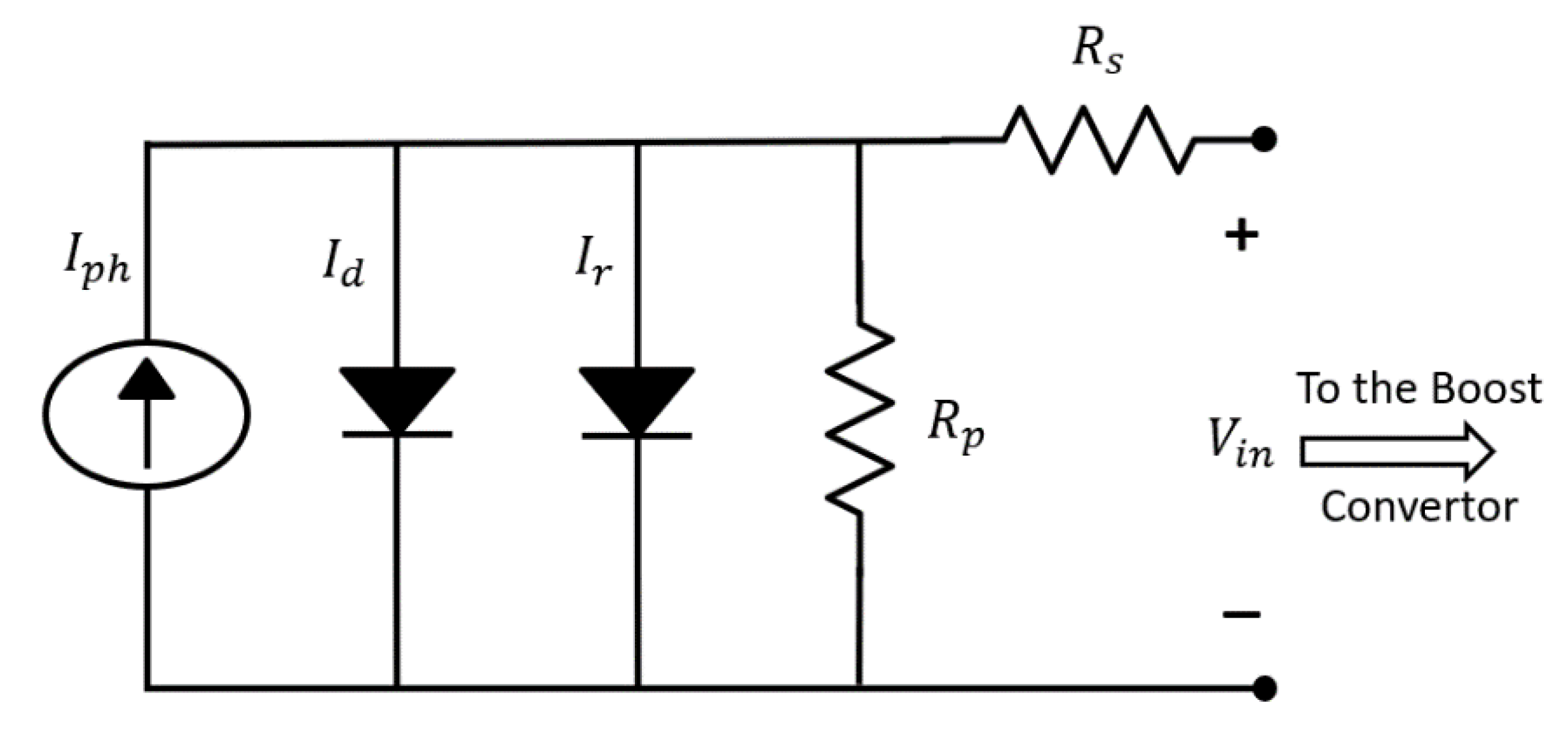
2. PV Mathematical Model

The amount of the harvested solar power is highly affected by the amount of solar radiations and temperature. For example, in Corpus Christi International Airport (CRP), TX, USA, the power received from sunlight at noon is more than the power received in the evening or morning as shown in Figure 1a [22]. As seen in Figure 1b [23], the ambient temperature changes month to month, and it can reach high values and cause a reduction in the PV conversion efficiency.

More precisely, the MPP changes with the ambient conditions, as shown in Figure 2, and there is need to have a controller that is capable of setting the PV load near the MPP. The controller design process basically relies on the PV cell’s modeling upon the interaction with the ambient conditions.

The mathematical modeling of a PV cell is derived in this section using the double diode PV structure, as shown in Figure 3.

The fundamental equation for the current generated in the photovoltaic cell is given in Equation (1), in which ($I_{ph})$ is the photovoltaic current formed by photons and ($I_{sc})$ is the short circuit current.

$$I_{ph}= \left(I_{sc}(1+\alpha \left(T-T_0\right)\right)\frac{S}{S_0}$$

(1)

where $\alpha$ is the cell’s short-circuit current temperature coefficient, $T$ is the temperature during the day, $T_0$ is the reference voltage (25 $℃$),$S$ is the irradiance during the day in W/m², and $S_0$ is the reference irradiance (1000 W/m²). The current $\left(I\right)$ generated by the double diode solar cell model is given as in Equation (2)

$$I=I_{ph}-I_0\times exp\left(\frac{V+I{R}_s}{n{V}_t} - 1\right)-I_r\times exp\left(\frac{V+I{R}_s}{n{V}_t} - 1\right)-\frac{V+I{R}_s}{R_p}$$

(2)

where $I_0$ is the reverse saturation current of the diode, $V$ is the PV output voltage, $V_t$ is the thermal voltage (25.85 mV at 300K), $R_s$ is the internal series resistance of the PV, $R_p$ is the internal parallel resistance of the PV, $I_r$ is the recombination current losses, and $n$ is the ideality factors with 1.5 value.

The MPP occurs when the rate of change of power to the voltage is zero, as shown in Figure 2a and is formulated as in Equation (3).

$$\frac{dP}{d{V}_{in}} \left\{\begin{array}{c}=0, at the MPP\\ > 0, at the left side of the MPP\\ < 0, at the right side of the MPP\end{array}\right\}$$

(3)

This equation will be used as the control law for the MPPT adaptive controller.

The next section shows the circuit design for a general Boost converter circuit with its mathematical model. This model is important in the controller design process.

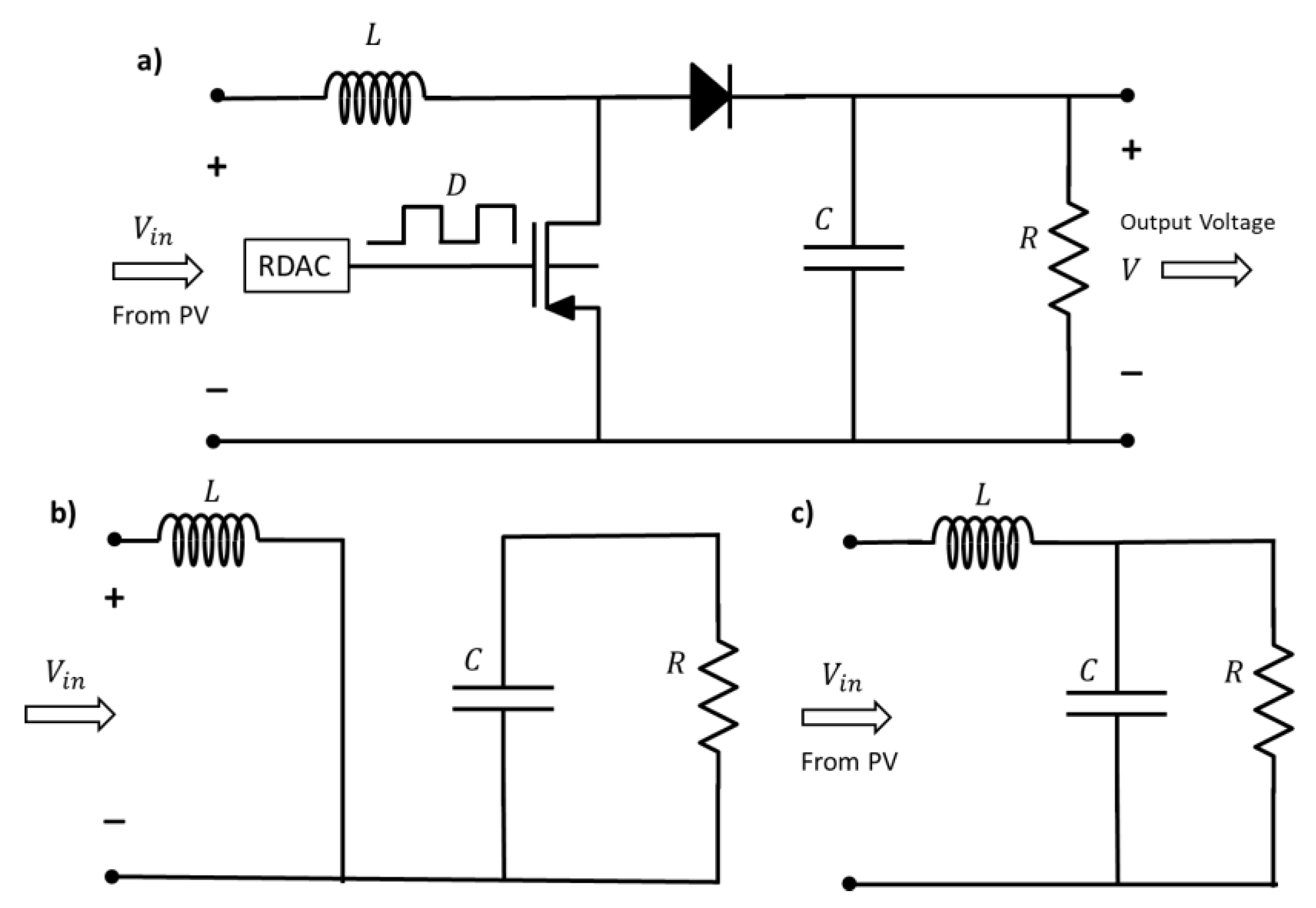
3. Boost Converter Model

Boost converter topology as shown in Figure 4 is used in this paper for the design of adaptive control algorithm to track the MPP, where D is the duty cycle, V is the boost converter output voltage, and R is the applied load. A combination of the capacitor (C) and the inductor (L) is used to minimize the current and voltage ripple at the output side. The boost converter average output voltage (V) is always higher than the PV’s voltage ($V_{in}$) as shown in Equation (4) due to: (a) The resistance of the inductor to change the current flowing inside it, and (b) the high switching frequency.

$$\frac{V_{in}}{V}=1- D$$

(4)

For the above system, and when the switch is closed as shown in Figure 4b, Kirchhoff’s voltage law is applied on the left side of the circuit to find the inductor current as in Equation (5) [24,25].

$${\left(\frac{{\mathrm{di}}_{\mathrm{L}}}{\mathrm{dt}}\right)}_{close}= \frac{V_{in}}{L}$$

(5)

Then, Kirchhoff’s current law is applied on the right side of the same circuit to find the capacitor voltage, which is the same as the output voltage

$${\left(\frac{\mathrm{dV}}{\mathrm{dt}}\right)}_{close}= -\frac{V}{RC}.$$

(6)

Likewise, Kirchhoff’s voltage and current laws are applied on the Boost converter circuit again, but this time when the switch is open, as shown in Figure 4c, to get the current and voltage equations as shown in Equations (7) and (8), respectively.

$${\left(\frac{{\mathrm{di}}_{\mathrm{L}}}{\mathrm{dt}}\right)}_{open}= \frac{1}{L}\left(V_{in}-V\right)$$

(7)

$${\left(\frac{\mathrm{dV}}{\mathrm{dt}}\right)}_{open}= \frac{1}{C}\left(i_L-\frac{V}{R}\right)$$

(8)

The average current and voltage values can be found by adding Equation (5) to Equation (7) and Equation (6) to Equation (8), respectively, as shown below

$$\frac{{\mathrm{di}}_{\mathrm{L}}}{\mathrm{dt}}=D{\left(\frac{{\mathrm{di}}_{\mathrm{L}}}{\mathrm{dt}}\right)}_{close}+ \left(1-D\right){\left(\frac{{\mathrm{di}}_{\mathrm{L}}}{\mathrm{dt}}\right)}_{open}$$

(9)

$$\frac{\mathrm{dV}}{\mathrm{dt}}=D{\left(\frac{\mathrm{dV}}{\mathrm{dt}}\right)}_{close}+ \left(1-D\right){\left(\frac{\mathrm{dV}}{\mathrm{dt}}\right)}_{open}.$$

(10)

After simplification, the average current and voltage are given in Equations (11) and (12), respectively.

$$\frac{{\mathrm{di}}_{\mathrm{L}}}{\mathrm{dt}}=\frac{V_{in}}{L}-\left(1-D\right) \frac{V}{L}$$

(11)

$$\frac{\mathrm{dV}}{\mathrm{dt}}=-\frac{V}{RC}+\left(1-D\right) \frac{{\mathrm{i}}_{\mathrm{L}}}{C}$$

(12)

which results in a combined form of

$$\left[\begin{array}{c}\frac{{\mathrm{di}}_{\mathrm{L}}}{\mathrm{dt}}\\ \frac{\mathrm{dV}}{\mathrm{dt}}\end{array}\right]=\left[\begin{array}{cc}0& -\frac{\left(1-D\right)}{L}\\ \frac{\left(1-D\right)}{C}& \frac{-1}{RC}\end{array}\right]\left[\begin{array}{c}{\mathrm{i}}_{\mathrm{L}}\\ \mathrm{V}\end{array}\right]+\left[\begin{array}{c}\frac{1}{L}\\ 0\end{array}\right]V_{in}.$$

(13)

A state space representation for Equation (13) can be obtained by setting the current as of the first state $x_1$ and the output voltage as a second state$x_2$. This state space representation is required to find the boost converter transfer function in the s-domain [26,27].

$${\dot{x}}_p\left(t\right)=\left[\begin{array}{c}{\dot{x}}_1\left(t\right)\\ {\dot{x}}_2\left(t\right)\end{array}\right]=A_p\left[\begin{array}{c}{x}_1\left(t\right)\\ x_2\left(t\right)\end{array}\right]+B_p{V}_{in}$$

(14)

$$y_p\left(t\right)=C_p\left[\begin{array}{c}{x}_1\left(t\right)\\ x_2\left(t\right)\end{array}\right]$$

(15)

$$A_p=\left[\begin{array}{cc}0& -\frac{\left(1-D\right)}{L}\\ \frac{\left(1-D\right)}{C}& \frac{-1}{RC}\end{array}\right]$$

(16)

$$B_p=\left[\begin{array}{c}\begin{array}{c}\frac{1}{L}\\ \end{array}\\ 0\end{array}\right]$$

(17)

where the matrices $A_p$ and $B_p$ represent the state and input matrices, respectively.

Finally, to find the boost converter transfer function in terms of the system input voltage $V_{in}$ and the output voltage V, the matrix $C_p$ is set to $\left[01\right]$ [28].

Using Equations (14) and (15), the boost converter transfer function $G_p\left(s\right),$can easily be found as given in Equation (19)

$$\frac{V\left(s\right)}{V_{in}\left(s\right)}=C_p\times {\left(\left[\begin{array}{cc}s& 0\\ 0& s\end{array}\right]-A_p\right)}^{-1}\times B_p$$

(18)

$$G_p\left(s\right)=\frac{R\left(1-D\right)}{RLC{s}^2+Ls+R{\left(1-D\right)}^2}.$$

(19)

The plant parameters R, L, and C are not constant and vary within the upper and lower range of their nominal values ($R^{*}, L^{*}, C^{*}$) as:

$$\begin{array}{c}{R}_{min}\le R*\le R_{max}\\ L_{min}\le L*\le L_{max}\\ C_{min}\le C*\le C_{max}\end{array}.$$

(20)

The purpose of this is to make sure that the controller can work for a wide range of load values (R), as well as to make sure that the controller can work with different sizes of the boost converters, which is represented by L and C.

Table 1. Ranges of values for the PV plant transfer function.

	$\mathbf{R}\left(\mathit{\Omega }\right)$	L (Henry)	C (Farad)
Nominal	15	0.8 × ${10}^{-3}$	1.0 × ${10}^{-3}$
Minimum	10	0.4 × ${10}^{-3}$	0.8 × ${10}^{-3}$
Maximum	18	1.2 × ${10}^{-3}$	1.2 × ${10}^{-3}$

below shows the ranges of values for each parameter of the system.

In the design, the boost converter capacitance and inductance values must be selected carefully to minimize the voltage and current ripples. To minimize the voltage ripples as proposed in [29], the capacitance is chosen such that

$$C\ge \frac{I}{f\Delta V}D$$

(21)

where $f$ is the switching frequency and $\Delta V$ is the voltage ripple. Estimating the voltage ripple factor as

$$VRF= \frac{\Delta V}{V}$$

(22)

To minimize the current ripple, again as proposed in [29], the inductance is chosen such that

$$L\ge \frac{V}{f\Delta I}D\left(D-1\right)$$

(23)

where $\Delta I$ is the current ripple which is given as,

$$CRF= \frac{\Delta I}{I}$$

(24)

where CRF is the current ripple factor. Based on the PV system parameters in

Table 2. System parameters of PV model, Boost converter, and robust direct adaptive controller (RDAC).

PV Model (at 25 C; 1000 W/m2)		Boost Converter		RDAC
$I_{sc}$	4.42 (A)	$CR{F}_{ }$	30%	$T_{pe}$	5.0 × ${10}^{-5}$
$V_{oc}$	44.35 (V)	$VR{F}_{ }$	5%	$T_{ie}$	1.0 × ${10}^{-5}$
$I_{max}$	3.84 (A)	$C^{ *}$	1000 $\mathsf{\mu }$F	$T_{pu}$	5.0 × ${10}^{-5}$
$V_{max}$	33.9 (V)	$L^{ *}$	0.8 mH	$T_{px}$	5.0 × ${10}^{-5}$
$P_{max}$	130 (W)	$R{ }^{*}$	15 $\mathsf{\Omega }$	$T_{ix}$	1.0 × ${10}^{-5}$
		Frequency	10 kHz	$T_{iu}$	1.0 × ${10}^{-5}$

, the minimum values of the inductance and capacitance must be greater than the maximum values shown in Figure 5 to satisfy Equations (21) and (23).

The next section shows the controller design step for the robust direct adaptive controller based on the physics of PV cells and based on the Boost converter topology for MPPT application.

4. Robust Direct Adaptive Control

Design of a robust direct adaptive controller (RDAC) is proposed to maximize the collected output power from PV systems. The overall block diagram of the proposed control system is illustrated in Figure 6. Here, MPPT control law refers to the use of Equation (3) where the maximum power occurs, and the controller reference voltage will vary according to the following equation, where $V$ is the Boost converter output voltage and $\Delta V$ is small threshold voltage.

$$V_{ref}= \{\begin{array}{c}V ,\raisebox{1ex}{$dP$}\!\left/ \!\raisebox{-1ex}{$d{V}_{in}$}\right.=0 \\ V-\Delta V,\raisebox{1ex}{$dP$}\!\left/ \!\raisebox{-1ex}{$d{V}_{in}$}\right.<0\\ V+\Delta V,\raisebox{1ex}{$dP$}\!\left/ \!\raisebox{-1ex}{$d{V}_{in}$}\right.>0\end{array}$$

(25)

Unless the feedback control, the adaptive control technique through the adaptation law can cope with disturbances, uncertainties in the system dynamics, as well as variations in operating conditions [30,31]. RDAC algorithm is developed for the MPP application because of its unique features and ease of implementation.

The proposed RDAC uses only the Boost converter inputs and outputs and does not need any estimations or identification of Boost converter parameters. The RDAC is composed mainly of a reference model, compensator, and three adaptive gains ($K_e, K_x, K_u$) [32] as shown in Figure 7, where $K_e$ is the adaptive gain of the error, $K_x$ is the adaptive gain of the states, and $K_u$ is the adaptive gain of the input, formulated as

$$D\left(t\right)=K_e\left(t\right)e_z\left(t\right)+K_x\left(t\right)x_m\left(t\right)+K_u\left(t\right)u_m\left(t\right)$$

(26)

where $e_z\left(t\right)$, $x_m\left(t\right)$, and $u_m\left(t\right)$ are the compensated error, the reference model states, and the input signals, respectively.

The main goal of RDAC is that the Boost converter (main plant) output $y_p\left(t\right)$ will follow the reference plant output $y_m\left(t\right)$ by use of the adaptive gains.

As described in [33,34], to implement the RDAC, the plant $G_p\left(s\right)$ has to be almost strictly positive real (ASPR), and if the plant $G_p\left(s\right)$ is not ASPR, then a compensator $G_c\left(s\right)$ has to be added in the feedforward path to the plant so that the new plant, called augmented plant $G_a\left(s\right)$, becomes ASPR, mathematically formulated as

$$G_a\left(s\right)= G_p\left(s\right)+G_c\left(s\right)= \frac{Z\left(s\right)}{T\left(s\right)}.$$

(27)

Simply said, the plant is an ASPR if the numerator polynomial of the plant transfer function is a minimum phase, the relative degree of the plant transfer function is 0 or 1, and the high-frequency gain (the coefficient of the highest numerator polynomial) is positive [35].

Based on the above ASPR conditions, it is clear that the Boost converter plant (Equation (19)) is not an ASPR and therefore a compensator in the feedforward path must be designed, which is presented in details below.

The Boost converter model is represented in the state-space representation for the RDAC design and is given in Equations (13)–(17). The first-order reference model was chosen to be used in the RDAC structure as below

$${\dot{x}}_m\left(t\right)= A_m{x}_m\left(t\right)+ B_m{u}_m\left(t\right)$$

(28)

$$y_m\left(t\right)= C_m{x}_m\left(t\right)$$

(29)

with model parameters being assumed as$A_m=\left[-10\right]$,$B_m=\left[1\right]$, and $C_m=\left[10\right]$.

The dimension of the model can be chosen freely as long as dim ($x_m$) $\le$ dim ($x_p$).

The RDAC output control signal is a periodic square wave with fixed frequency and with variable duty cycle ($D\left(t\right)$) that will send the Boost converter operating voltage to the MPP. For the characteristic of the output, the first-order model seems to be sufficient.

The adaptive control signal, $D\left(t\right)$ is given as

$$D\left(t\right)= \left|k_e\left(t\right)e_z\left(t\right)\right|+\left|k_x\left(t\right)x_m\left(t\right)\right|+\left|k_u\left(t\right)u_m\left(t\right)\right|$$

(30)

where $e_z\left(t\right)$ is the compensated error and equals to ($y_r\left(t\right)-y_a\left(t\right)$). Absolute condition is applied in Equation (30) to make sure that $D\left(t\right)$ is greater than 0.

Although a compensator output was added to both reference model and plant output resulting in an error $e_z\left(t\right)$, it has been shown that as $e_z\left(t\right)$ goes to zero, $e_y\left(t\right)=y_p\left(t\right)-y_m\left(t\right)$ goes to zero; therefore, we only consider$e_y\left(t\right)$. For ease of derivations, vector $r^T\left(t\right)$ can be defined as:

$$r^T\left(t\right)={[}_{ }{e}_{ }{}_z^T\left(t\right) x_{ }{}_m^T\left(t\right) u_{ }{}_m^T\left(t\right)].$$

(31)

According to [36], each adaptive gain of$K_{ }\left(t\right)=\left[K_e\left(t\right) K_x\left(t\right) K_u\left(t\right)\right]$consists of two parts; proportional and integral parameters and as described in the following equations, where $T_p$ and $T_i$ are the proportional weight constant and integral weight constant, respectively:

$$K_{ }\left(t\right)= K_p\left(t\right)+ K_i\left(t\right)$$

(32)

$$K_p\left(t\right)=e_z\left(t\right)\times r^T\left(t\right)\times T_p, T_p\ge 0$$

(33)

$$\dot{K_i}\left(t\right)=e_z\left(t\right)\times r^T\left(t\right)\times T_i, T_i>0.$$

(34)

$T_p$ is a vector that contains three constants $\left[\begin{array}{ccc}{T}_{pe}& T_{px}& T_{pu}\end{array}\right]$; likewise, $T_i$ is a vector and contains three constants $\left[\begin{array}{ccc}{T}_{ie}& T_{ix}& T_{iu}\end{array}\right]$.

Since the Boost converter plant model is formed by physical parameters; the resistance ($R)$, the inductance $\left(L\right)$, and the capacitance $\left(C\right)$ as demonstrated in Equation (19) change within a range between minimum and maximum limits while operating as described in (20). These limits must be taken into consideration to guarantee the stability and robustness of the system. The nominal transfer function of the system,$G_p{\left(s\right)}_{ }{}^{*}$ is given with nominal parameters as below

$$G_p{\left(s\right)}_{ }{}^{*}=\frac{R^{*}\left(1-D\right)}{\left(R^{*}{L}^{*}{C}^{*}\right)s^2+L^{*}s+R^{*}{\left(1-D\right)}^2}.$$

(35)

The difference between the nominal and the changing/unknown PV plant transfer functions could be modeled as an additive perturbation as in [36]

$${\Delta }_a{\left(s\right)}_{ }=G_p{\left(s\right)}_{ }-G_p{\left(s\right)}_{ }{}^{*}.$$

(36)

Now, the primary objective is to ensure the stability of the PV plant system, which is subject to the system parameters limits/constraints (Equation (20)) under the influence of the additive perturbations by modeling the uncertainties at the frequency domain. Since the ${\Delta }_a(j\omega$) is a function of plant parameters, to increase the range for the robustness of the system, it is clear that the ${\Delta }_a{\left(j\omega \right)}_{ }$ must be maximized at each frequency, i.e., one can write that

$$\underset{\zeta }{maximize }\left|{\Delta }_a{\left(j\omega \right)}_{ }\right| \forall \omega$$

(37)

$$\mathrm{Subject}\mathrm{to}:\{\begin{array}{c}{R}_{min}\le R*\le R_{max}\\ L_{min}\le L*\le L_{max}\\ C_{min}\le C*\le C_{max}\end{array}.$$

Once the perturbations are maximized at each frequency, it is necessary to define a bounding function for the extreme uncertainty case. This function, $W\left(s\right)\in R{H}_{\infty }$could be defined at the frequency domain as

$$\left|W\left(j\omega \right)\right|\ge max \left|{\Delta }_a{\left(j\omega \right)}_{ }\right| \forall \omega .$$

(38)

The compensator can now be designed according to the following design steps [36]:

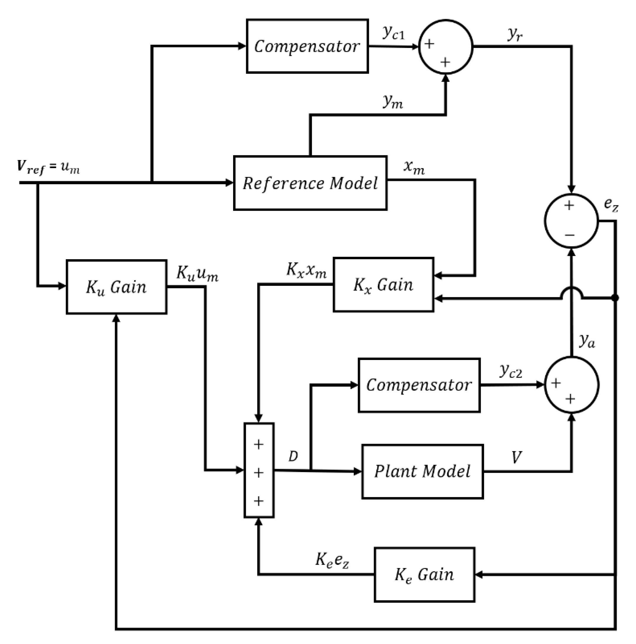
• The compensator transfer function must be stable with a desired relative degree of either 0 or 1.
• The closed-loop nominal plant transfer function of the system, $G_p{\left(s\right)}_{ }{}^{*},$ must be stable as well.
• $\tilde{\Delta }\left(s\right)\in R{H}_{\infty } \& {\left|\left|\tilde{\Delta }\left(s\right)\right|\right|}_{\infty }<1$, where $\tilde{\Delta }\left(s\right)$ is given in the following

  $$\tilde{\Delta }\left(s\right)= \frac{W\left(s\right)}{G_p{\left(s\right)}_{ }{}^{*}+G_c\left(s\right)}.$$

  (39)

The maximum perturbation and the bounding function after implementing the optimization formulation of Equation (38) is as shown in Equation (39) and as shown in Figure 8. Based on the maximum perturbations, it is desired to set the bounding function as

$$W\left(s\right)= \frac{s+14\times {10}^8}{s^2+4602 s+5.309\times {10}^6}.$$

(40)

In this case, the compensator’s generic transfer function$G_c\left(s\right)$ is chosen to be the following:

$$G_c\left(s\right)= \frac{f_1{s}^{ }+f_0}{h_2{s}^2{}^{ }+h_1{s}^{ }+h_0}.$$

(41)

It is noticeable from Equation (41) that the relative degree for the compensator’s transfer function is 1. Also, the unknown values of $f_1, f_0, h_2, h_1$, and $h_0$ are to be optimized. It is also important to note that the third condition ${\left|\left|\tilde{\Delta }\left(s\right)\right|\right|}_{\infty }<1$, of the above steps, is an optimization problem that requires minimization of the ${\left|\left|\tilde{\Delta }\left(s\right)\right|\right|}_{\infty }.$ The optimization problem could be formulated as

$$\underset{x}{minimize }{\left|\left|\tilde{\Delta }\left(s\right)\right|\right|}_{\infty }.$$

(42)

Subject to: $Real\left(roots\left(Z^{*}\left(s\right)\right)\right)<0$.

${\left|\left|\tilde{\Delta }\left(s\right)\right|\right|}_{\infty }$ is a function of $(f_1,f_0, h_2,h_{1}and h_0)$, $x$ is a vector of compensator parameters, and $Z^{*}\left(s\right)$ is the zero polynomial of the augmented nominal plant, $G_a{\left(s\right)}_{ }{}^{*}$.

$$G_a{\left(s\right)}_{ }{}^{*}= G_p{\left(s\right)}_{ }{}^{*}+G_c\left(s\right)= \frac{Z^{*}\left(s\right)}{T^{*}\left(s\right)}$$

(43)

After the optimization formulation of Equation (42) is implemented, the following compensator was obtained:

$$G_c\left(s\right)= \frac{7.2s+1.6}{s^2+s+1}.$$

(44)

Now that the design of the RDAC controller is done, the next section presents the results.

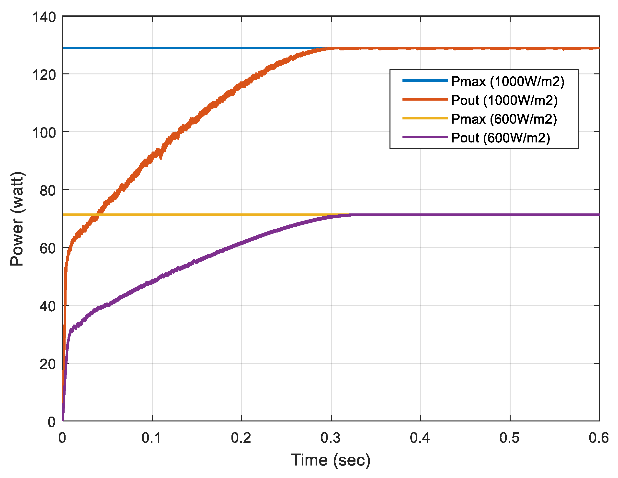
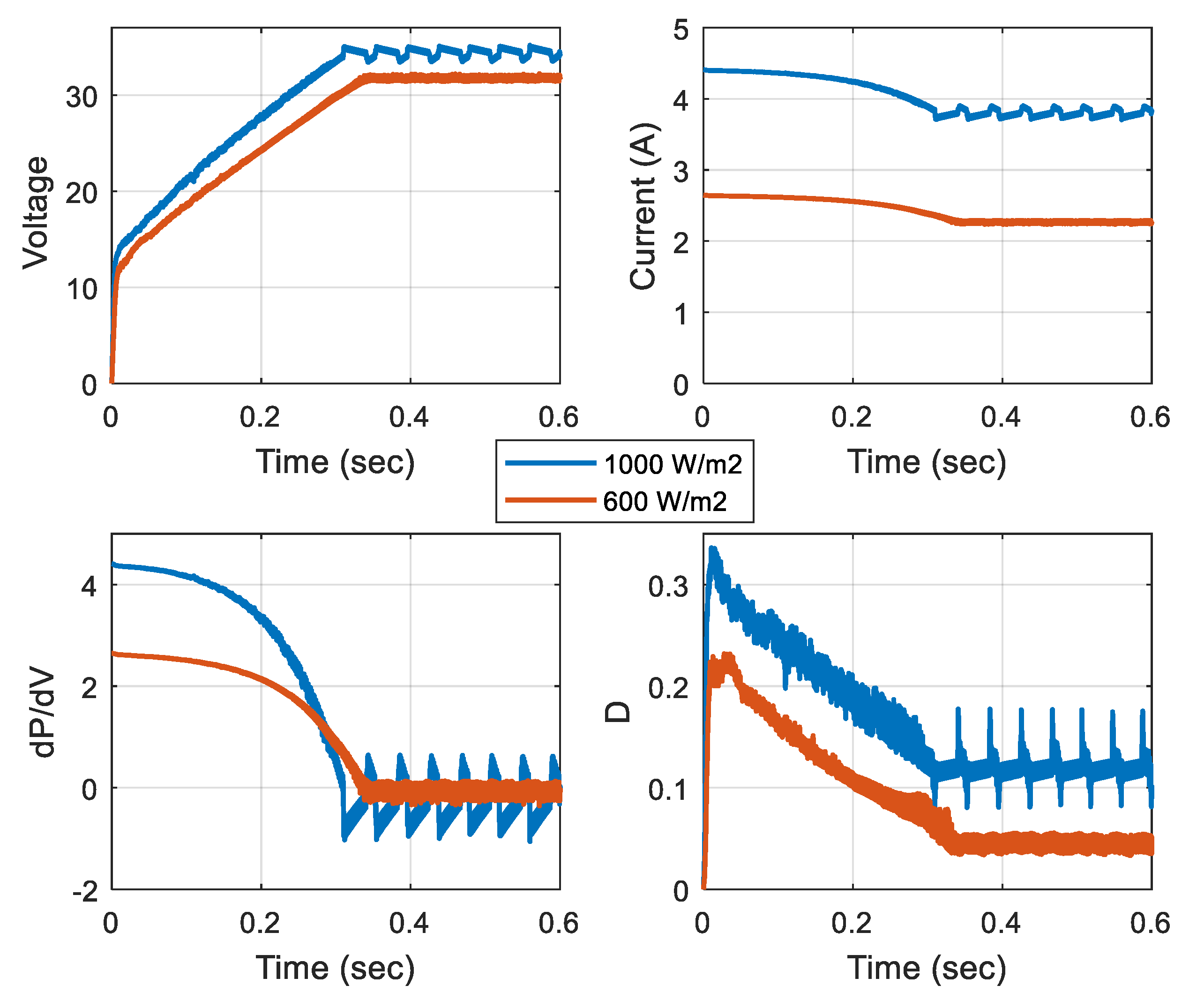
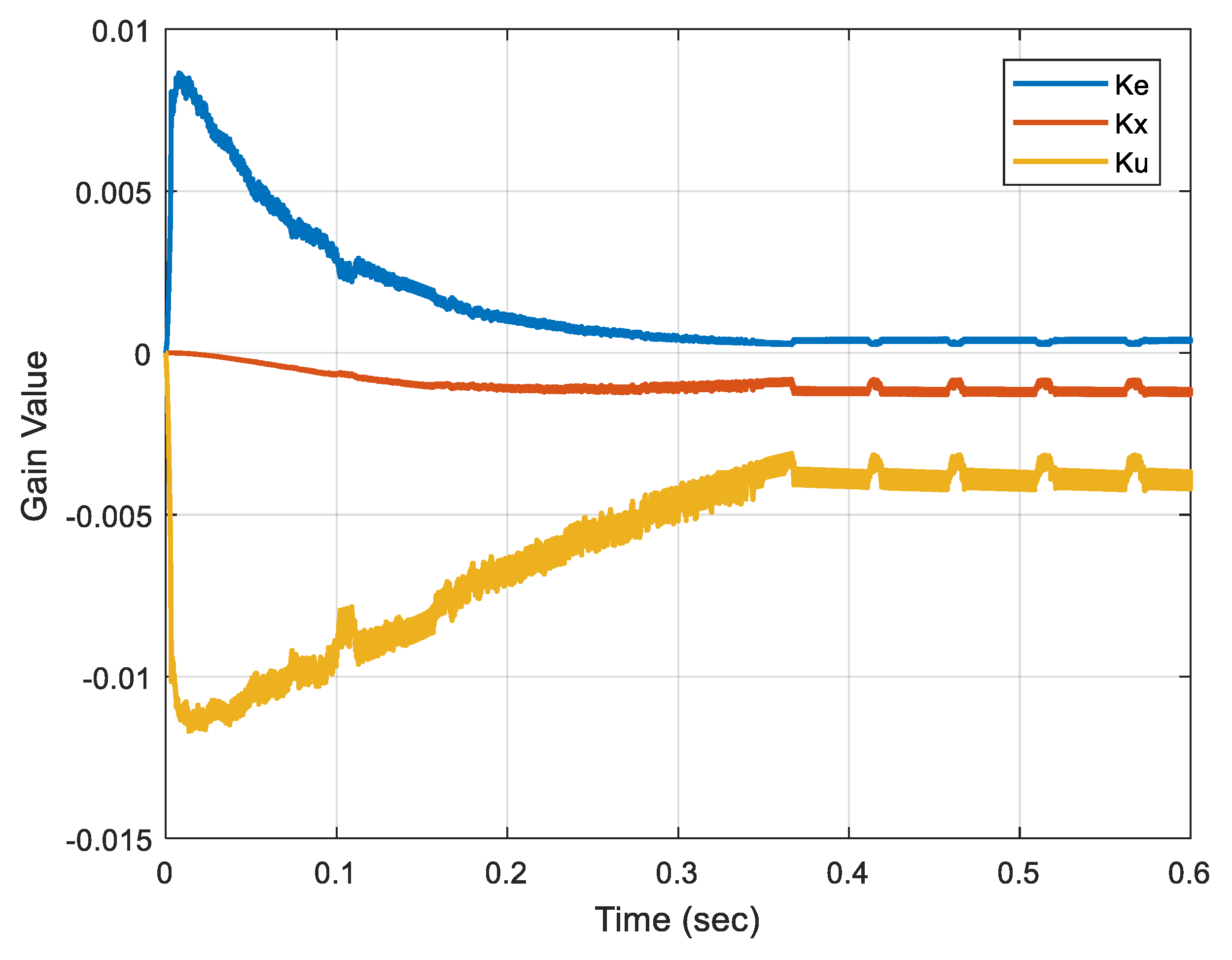
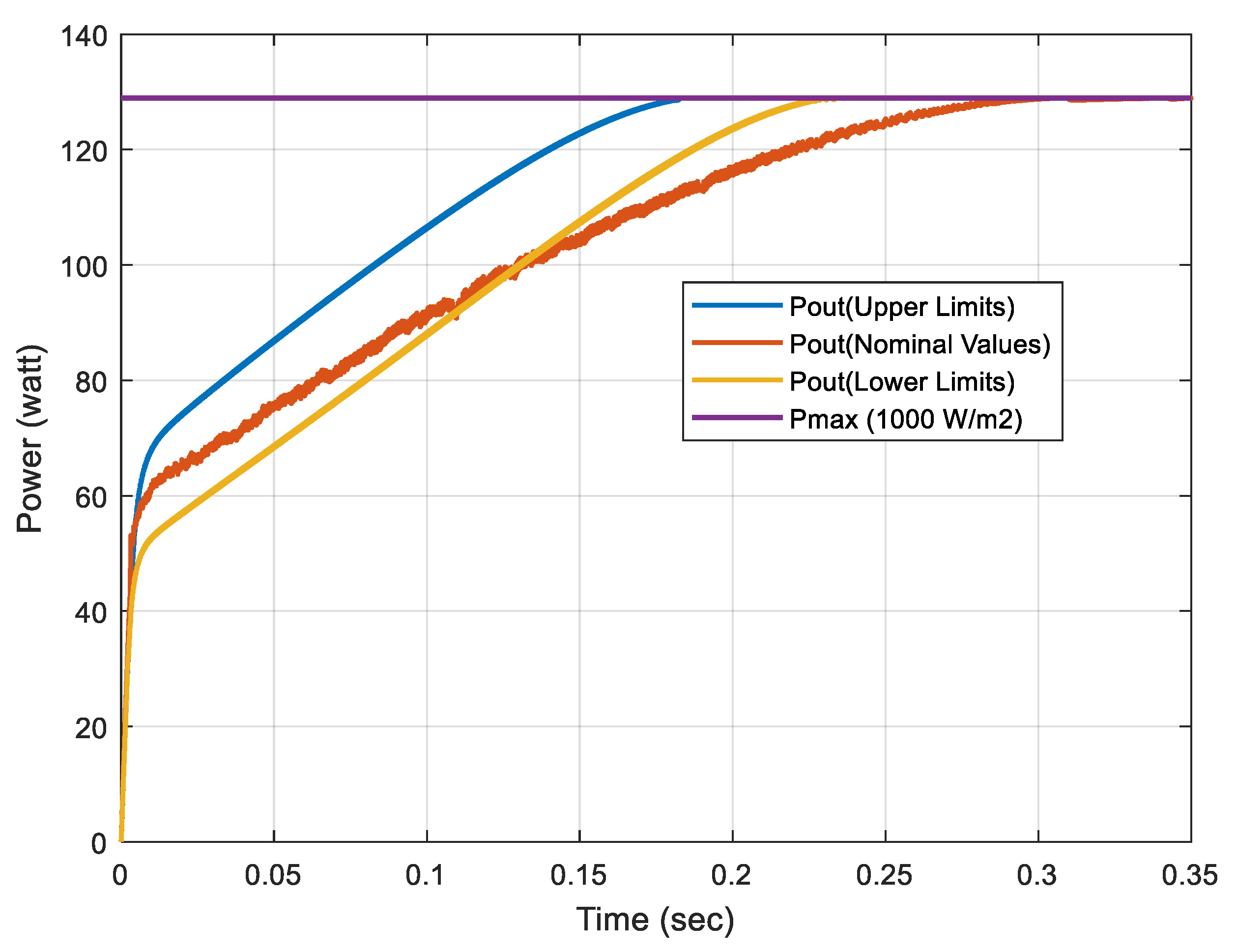
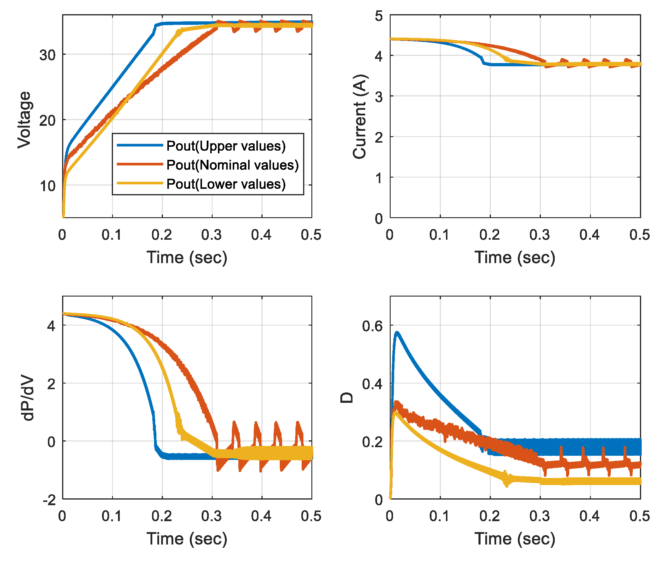
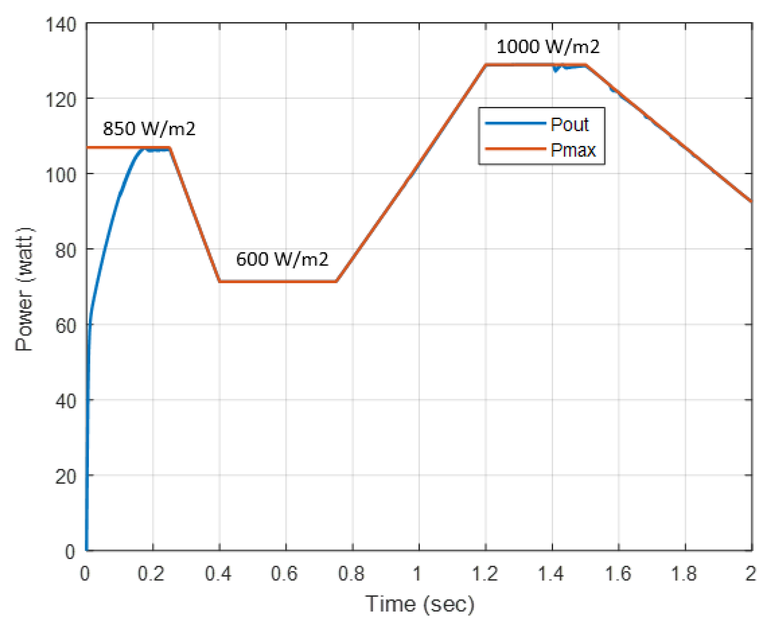
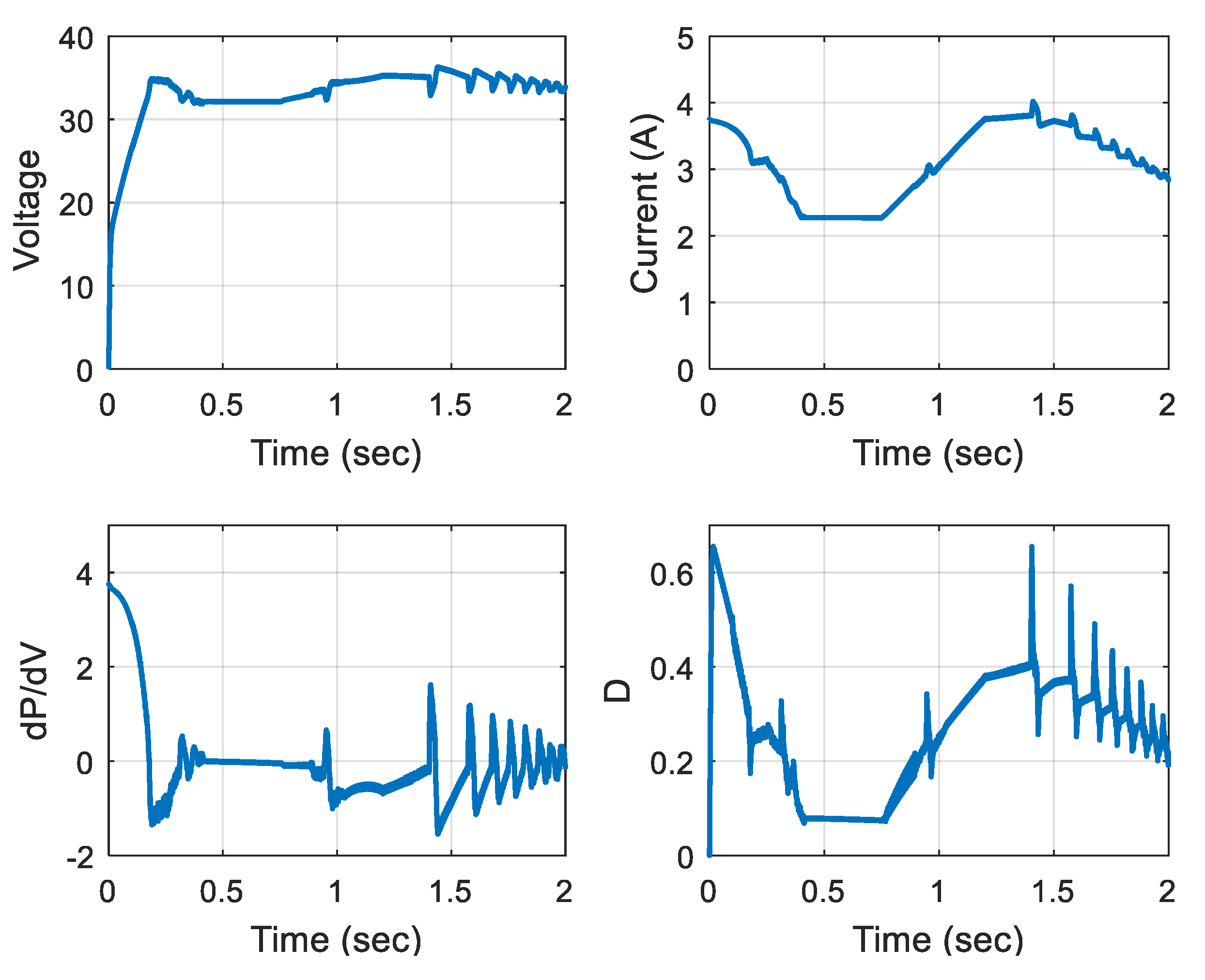
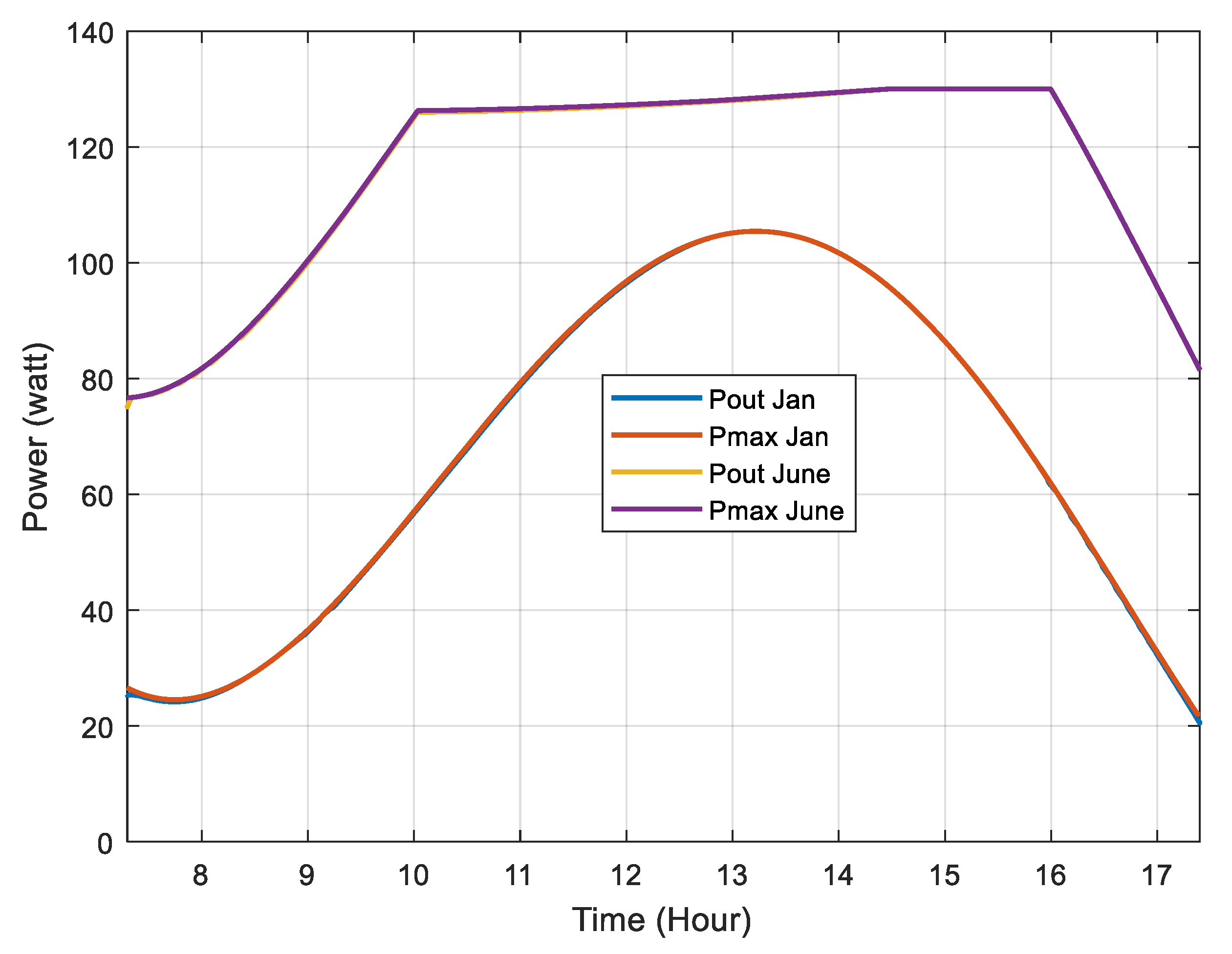
5. Results

The simulation for the MPPT with the RDAC was carried out using MATLAB/SIMULINK toolbox [37]. The simulation consists of three main components integrated together; the PV model, boost converter model, and the adaptive controller, where the process of operation is given in Figure 9 for the parameters given in Table 2.

Figure 10 shows the MPPT output power versus the expected maximum power for the PV cell (130 W) as in Table 2 for 1000 W/m² irradiance at 25$℃$. The results show that the response time for the adaptive controller is less than 0.3 s, which is faster than any other controller like in [38,39]. Also, the adaptive controller shows that it is capable of tracking the MPP for other irradiance values like 600 W/m², as shown in Figure 10 and Figure 11.

During the steady-state operation, there are some large peaks that occur in the duty cycle because of the high steady-state at the beginning of the RDAC operation, as shown in Figure 11.

Figure 12 shows the adaptive gain values that change with time, as expected.

In another simulation, the robustness of the adaptive controller was tested with different boost converter inductance and capacitance values, as shown in Table 1. Figure 13 illustrates the output results for power. The controller can adapt to the changes within the boost converter parameters, i.e., the controller algorithm presented in this paper can be used with different MPPT types, and it will lead to a stable system and maximum output power values, as shown in Figure 14.

Furthermore, the controller’s performance was tested at different irradiance values with ramp variations, as shown in Figure 15 and Figure 16. These variations may be interpreted as different weather conditions and are important to validate the controller’s efficiency at cloudy or dusty weather, for example.

The real irradiance and temperature values in Figure 1 were used to test the controller’s performance for the real-life scenario at a typical summer and winter sunny days, in this case, 1 June and 1 January, respectively, as shown in Figure 17. The simulation was done based on an hourly basis to test the adaptive controller for long-time operations. For the month of June’s case, the output power is clamped between 10:00 and 16:00 because the solar cell in this simulation can produce up to its maximum power at 1000 W/m² and 25 $℃$.

Figure 18 shows the current, voltage, $dP/dV$, and duty cycle results for June and January cases.

Figure 18 shows the current and voltage for a typical day in summer and winter at which the sun’s radiations are varying with the temperature. The controller tries to keep track for the MPP with these variations in radiations and temperature.

6. Conclusions

Adaptive control algorithms have been used widely in the nonlinear or time-varying processes because of their ability to deal with the unexpected changes in the system dynamics or inputs. Also, adaptive controllers required less processing time and less pre-knowledge about the system. This paper presents the using of robust direct adaptive controller that can set the PV output voltage at the maximum power point as shown in the previous results, and hence, more power can be harvested from the PV system. Besides, RDAC shows better performance in the tracking of the MPP at different boost converter parameters (L,C), and at different operating conditions, which is unique thing compared to other types of controllers. The Boost converter design is important to minimize the ripple voltage; however, RDAC helps in maintaining low variation in the output voltage and near the MPP. The adaptive controller compensator design is an essential thing to improve the controller robustness. The RDAC design can be improved in the future to include other renewable energy-related applications like the MPPT from wind turbines.

References

- Knuth, S. ‘Breakthroughs’ for a green economy? Financialization and clean energy transition. Energy Res. Soc. Sci. 2018, 41, 220–229. [Google Scholar] [CrossRef]
- Ramanujam, J.; Verma, A.; González-Díaz, B.; Guerrero-Lemus, R.; del Cañizo, C.; García-Tabarés, E.; Rey-Stolle, I.; Granek, F.; Korte, L.; Tuccih, M.; et al. Inorganic photovoltaics—Planar and nanostructured devices. Prog. Mater. Sci. 2016, 82, 294–404. [Google Scholar] [CrossRef]
- Kumar, M.; Kumar, A. Performance assessment and degradation analysis of solar photovoltaic technologies: A review. Renew. Sustain. Energy Rev. 2017, 78, 554–587. [Google Scholar] [CrossRef]
- Creutzig, F.; Agoston, P.; Goldschmidt, J.C.; Luderer, G.; Nemet, G.; Pietzcker, R.C. The underestimated potential of solar energy to mitigate climate change. Nat. Energy 2017, 2, 17140. [Google Scholar] [CrossRef]
- Salim, M.B.; Demirocak, D.E.; Barakat, N. A Fuzzy Based Model for Standardized Sustainability Assessment of Photovoltaic Cells. Sustainability 2018, 10, 4787. [Google Scholar] [CrossRef]
- Fthenakis, V.M.; Kim, H.C. Photovoltaics: Life-cycle analyses. Sol. Energy 2011, 85, 1609–1628. [Google Scholar] [CrossRef]
- Shafeey, M.A.; Harb, A.M. Photovoltaic as a promising solution for peak demands and energy cost reduction in Jordan. In Proceedings of the 2018 9th International Renewable Energy Congress (IREC), Hamment, Tunisia, 20–22 March 2018; pp. 1–4. [Google Scholar]
- Gules, R.; Pacheco, J.D.P.; Hey, H.L.; Imhoff, J. A Maximum Power Point Tracking System with Parallel Connection for PV Stand-Alone Applications. IEEE Trans. Ind. Electron. 2008, 55, 2674–2683. [Google Scholar] [CrossRef]
- Jordan, D.C.; Silverman, T.J.; Wohlgemuth, J.H.; Kurtz, S.R.; VanSant, K.T. Photovoltaic failure and degradation modes. Prog. Photovolt. Res. Appl. 2017, 25, 318–326. [Google Scholar] [CrossRef]
- Li, L.; Wang, H.; Chen, X.; Bukhari, A.A.S.; Cao, W.; Chai, L.; Li, B. High Efficiency Solar Power Generation with Improved Discontinuous Pulse Width Modulation (DPWM) Overmodulation Algorithms. Energies 2019, 12, 1765. [Google Scholar] [CrossRef]
- Pathy, S.; Subramani, C.; Sridhar, R.; Thentral, T.M.T.; Padmanaban, S. Nature-Inspired MPPT Algorithms for Partially Shaded PV Systems: A Comparative Study. Energies 2019, 12, 1451. [Google Scholar] [CrossRef]
- Espi, J.M.; Castello, J. A Novel Fast MPPT Strategy for High Efficiency PV Battery Chargers. Energies 2019, 12, 1152. [Google Scholar] [CrossRef]
- Cortajarena, J.A.; Barambones, O.; Alkorta, P.; de Marcos, J. Sliding mode control of grid-tied single-phase inverter in a photovoltaic MPPT application. Sol. Energy 2017, 155, 793–804. [Google Scholar] [CrossRef]
- Kolsi, S.; Samet, H.; Amar, M.B. Design Analysis of DC-DC Converters Connected to a Photovoltaic Generator and Controlled by MPPT for Optimal Energy Transfer throughout a Clear Day. J. Power Energy Eng. 2014, 2, 27. [Google Scholar] [CrossRef]
- Tran, C.H.; Nollet, F.; Essounbouli, N.; Hamzaoui, A. Modeling and Simulation of Stand Alone Photovoltaic System using Three Level Boost Converter. In Proceedings of the 2017 International Renewable and Sustainable Energy Conference (IRSEC), Tangier, Morocco, 4–7 December 2017; pp. 1–6. [Google Scholar]
- Ahmed, M.E.; Mousa, M.; Orabi, M. Development of high gain and efficiency photovoltaic system using multilevel boost converter topology. In Proceedings of the 2nd International Symposium on Power Electronics for Distributed Generation Systems, Hefei, China, 16–18 June 2010; pp. 898–903. [Google Scholar]
- Anto, E.K.; Asumadu, J.A.; Okyere, P.Y. PID control for improving P amp; amp; O-MPPT performance of a grid-connected solar PV system with Ziegler-Nichols tuning method. In Proceedings of the 2016 IEEE 11th Conference on Industrial Electronics and Applications (ICIEA), Hefei, China, 5–7 June 2016; pp. 1847–1852. [Google Scholar]
- Kermadi, M.; Berkouk, E.M. Artificial intelligence-based maximum power point tracking controllers for Photovoltaic systems: Comparative study. Renew. Sustain. Energy Rev. 2017, 69, 369–386. [Google Scholar] [CrossRef]
- Hohm, D.P.; Ropp, M.E. Comparative study of maximum power point tracking algorithms. Prog. Photovolt. Res. Appl. 2003, 11, 47–62. [Google Scholar] [CrossRef]
- Dahmane, M.; Bosche, J.; El-Hajjaji, A.; Pierre, X. MPPT for photovoltaic conversion systems using genetic algorithm and robust control. In Proceedings of the American Control Conference, Washington, DC, USA, 17–19 June 2013; pp. 6595–6600. [Google Scholar]
- Wu, Z.; Yu, D. Application of improved bat algorithm for solar PV maximum power point tracking under partially shaded condition. Appl. Soft Comput. 2018, 62, 101–109. [Google Scholar] [CrossRef]
- The National Renewable Energy Laboratory. NSRDB: Alphabetical List by State. Available online: https://rredc.nrel.gov/solar/old_data/nsrdb/1991-2010/hourly/list_by_state.html (accessed on 8 December 2018).
- IOWA State University, IOWA environmental Mesonet. IEM: Download ASOS/AWOS/METAR Data. Available online: https://mesonet.agron.iastate.edu/request/download.phtml?network=TX_ASOS (accessed on 8 December 2018).
- Shabrina, H.N.; Setiawan, E.A.; Sabirin, C.R. Designing of new structure PID controller of boost converter for solar photovoltaic stability. In Proceedings of the International Tropical Renewable Energy Conference (i-TREC) 2016 on Renewable Energy Technology and Innovation for Sustainable Development, Bogor, Indonesia, 26–28 October 2017; p. 020026. [Google Scholar]
- Husna, A.W.N.; Siraj, S.F.; Muin, M.Z.A. Modeling of DC-DC converter for solar energy system applications. In Proceedings of the 2012 IEEE Symposium on Computers Informatics (ISCI), Penang, Malaysia, 18–20 March 2012; pp. 125–129. [Google Scholar]
- Priewasser, R.; Agostinelli, M.; Unterrieder, C.; Marsili, S.; Huemer, M. Modeling, Control, and Implementation of DC–DC Converters for Variable Frequency Operation. IEEE Trans. Power Electron. 2014, 29, 287–301. [Google Scholar] [CrossRef]
- Mira, M.C.; Knott, A.; Thomsen, O.C.; Andersen, M.A.E. Boost converter with combined control loop for a stand-alone photovoltaic battery charge system. In Proceedings of the 2013 IEEE 14th Workshop on Control and Modeling for Power Electronics (COMPEL), Salt Lake City, UT, USA, 23–26 June 2013; pp. 1–8. [Google Scholar]
- Zhang, W.; Tan, X.; Wang, K.; Li, T.; Chen, J. Design for boost DC-DC converter controller based on state-space average method. Integr. Ferroelectr. 2016, 172, 152–159. [Google Scholar] [CrossRef]
- Mohammed, S.S.; Devaraj, D. Simulation and analysis of stand-alone photovoltaic system with boost converter using MATLAB/Simulink. In Proceedings of the 2014 International Conference on Circuits, Power and Computing Technologies (ICCPCT-2014), Nagercoil, India, 20–21 March 2014; pp. 814–821. [Google Scholar]
- Landau, I.D.; Lozano, R.; M’Saad, M.; Karimi, A. Introduction to Adaptive Control. In Adaptive Control; Springer: London, UK, 2011; pp. 1–33. [Google Scholar]
- Tariba, N.; Haddou, A.; Omari, H.E.; Omari, H.E. Design and implementation an Adaptive Control for MPPT systems using Model Reference Adaptive Controller. In Proceedings of the 2016 International Renewable and Sustainable Energy Conference (IRSEC), Marrakech, Morocco, 14–17 November 2016; pp. 165–172. [Google Scholar]
- Ozcelik, S.; DeMarchi, J.; Kaufman, H.; Craig, K. Control of an Inverted Pendulum Using Direct Model Reference Adaptive Control. IFAC Proc. Volumes 1997, 30, 585–590. [Google Scholar] [CrossRef]
- Bar-Kana, I.; Kaufman, H. Global Stability and Performance of a Simplified Adaptive Algorithm. Int. J. Control 1985, 46, 1491–1505. [Google Scholar] [CrossRef]
- Livnch, R.; McLaren, M.D.; Slater, G.L. Some conditions for almost strict positive realness. In Proceedings of the 29th IEEE Conference on Decision and Control, Honolulu, HI, USA, 5–7 December 1990; pp. 2512–2517. [Google Scholar]
- Iwai, Z.; Mizumoto, I. Robust and simple adaptive control systems. Int. J. Control 1992, 55, 1453–1470. [Google Scholar] [CrossRef]
- Kaufman, H.; Barkana, I.; Sobel, K. Direct Adaptive Control Algorithms: Theory and Applications, 2nd ed.; Springer: New York, NY USA, 1998. [Google Scholar]
- MATLAB—MathWorks. Available online: https://www.mathworks.com/products/matlab.html (accessed on 25 May 2019).
- Koofigar, H.R. Adaptive robust maximum power point tracking control for perturbed photovoltaic systems with output voltage estimation. ISA Trans. 2016, 60, 285–293. [Google Scholar] [CrossRef]
- Hasanien, H.M. An Adaptive Control Strategy for Low Voltage Ride Through Capability Enhancement of Grid-Connected Photovoltaic Power Plants. IEEE Trans. Power Syst. 2016, 31, 3230–3237. [Google Scholar] [CrossRef]