Evaluation of Contribution of PV Array and Inverter Configurations to Rooftop PV System Energy Yield Using Machine Learning Techniques

Abstract

Rooftop photovoltaics (PV) systems are attracting residential customers due to their renewable energy contribution to houses and to green cities. However, customers also need a comprehensive understanding of system design configuration and the related energy return from the system in order to support their PV investment. In this study, the rooftop PV systems from many high-volume installed PV systems countries and regions were collected to evaluate the lifetime energy yield of these systems based on machine learning techniques. Then, we obtained an association between the lifetime energy yield and technical configuration details of PV such as rated solar panel power, number of panels, rated inverter power, and number of inverters. Our findings reveal that the variability of PV lifetime energy is partly explained by the difference in PV system configuration. Indeed, our machine learning model can explain approximately $31\%$ ($95\%$ confidence interval: 29–38%) of the variant energy efficiency of the PV system, given the configuration and components of the PV system. Our study has contributed useful knowledge to support the planning and design of a rooftop PV system such as PV financial modeling and PV investment decision.

1. Introduction

The rooftop PV system is usually the first choice investment for the domestic application of customers when they consider following any renewable energy plans [1,2,3]. This system not only helps to reduce the monthly electric bill but also maximizes their profit by storing and selling energy back to the utility company. From the utility company’s perspective, the PV system, which operates as a distributed generation, can help the utility through many smart grid applications such as a demand response program, peak load shifting or net metering. Therefore, the development of a PV system at the customer scale should be encouraged with both technical and academic help.

The PV financial models and PV investment calculation are two common approaches to consider in a PV project plan. For instance, the meta-analysis in References [4,5,6] surveyed many popular PV financial models, considering the technical characteristic of PV component, PV configuration and type of solar panels. These studies helped a customer to choose a reliable tool for PV planning and design from the system point of view, without depending on the equipment supplier. The authors of References [7,8,9] studied the PV cost of the residential application of a PV system in terms of energy payback time (EPBT) and energy return on energy investment (EROI). They found that the small PV modules area helps to increase the energy yield but it increases the model-level and system-level cost per watt. From the geospatial perspective, the studies and simulation tools in References [10,11,12,13,14,15] estimated the effects of solar radiation, air temperature and wind speed to the PV energy yield. Unfortunately, their geospatial data are interpolated partly from satellite measurements, which reduces the reliability of the resulting model. Finally, the authors of Reference [16] recommended that customers consider a common DC bus of inverter configuration and an oversized PV array for their PV system in order to minimize the levelized cost of energy (LCOE).

Although the aforementioned literature has confirmed the effects of PV system configuration, PV components characteristics and geospatial data on the energy yield, they have failed to address the quantitative contribution of each factor to the overall energy result. A major reason is due to the lack of field data of rooftop PV systems. Indeed, many studies on PV systems are only validated locally, such as in Thailand [17] or Abu Dhabi [18,19]. In this research, we have collected 6729 rooftop PV systems from many countries and areas over the world that have a high-volume of installed PV systems from the pvoutput.org database [20] to conduct a quantitative evaluation of PV system configuration and component contributions to energy yield. In detail, we answer three following questions: (i) Is there any significant difference in energy yield caused by the inverter brands? (ii) Is there any significant difference between the two PV inverter configurations—micro-inverter and string inverter? and (iii) How much is the contribution, as a percentage, of PV system configuration and components to the PV energy yield? Answering the aforementioned questions will help the homeowner to choose the appropriate components and configuration for their PV investment. This study also contributes to a comprehensive understanding of rooftop PV characteristics to build a more accurate PV financial model.

The remainder of this paper is organized as follows. Section 2 presents the PV dataset that we gathered from pvoutput.org and the defined lifetime energy efficiency calculations. Section 3 introduces the method of applied machine learning that we have used in our study. Section 4 shows the resulting energy evaluation from the gathered PV dataset and our discussion. Finally, we conclude our study and state further research in Section 5.

2. Pv System Dataset

2.1. Description of Pv System Dataset

In this study, we have collected rooftop PV systems from pvoutput.org [20]. Currently, this is the biggest dataset about rooftop PV systems all over the world. It allows any users of a PV system to upload every 5-min measurement of power and energy that is generated by their system. The PV systems on this website are usually at the residential scale with a rated power of PV array lower than 5 kW peak.

Table 1. Specifications of PV systems at pvoutput.org website.

PV System		Example Values
Number of Panels		4; 8; 10; 12; 20; 26
Panel Max Power		165 W; 220 W; 275 W
System Size		3.24 kW; 4.9 kW; 9.82 kW
Panel Brand/Model		LG; Yingli; Solar Frontier; Sanyo
Orientation		North; South; West; East
Number of Inverters		1; 2; 3; 4
Inverter Brand/Model		SMA; Enphase; Solar Edge
Inverter Size		215 W; 500 W; 5000 W
Post Code		Belgium 2440; USA 94550
Installed Date		12/12/15
Shading		No; Low; Medium; High
Tilt degree		1; 18; 35; 45

describes some specifications of PV systems at the pvoutput.org source. From these registered data, we easily extract some useful information about the PV system, such as the system’s used string-inverter type or micro-inverter type, the rated power of solar panel and inverter and the shading condition of the PV system.

From Table 1, we can infer the characteristics of a PV system based on the recommendation of the Solar Bankability [21].

• Solar panel configuration: the number of solar panels; the rated panel power;
• Inverter configuration: the number of inverters, the rated inverter power;
• Geospatial dataset: orientation, tilt, region, shading condition.

2.2. Our Assumptions

The lifetime energy yield of a PV system is a key parameter that determines the profit of PV investment but is one of the least understood issues in the community. In our study, we define the lifetime energy yield $Y_L$ (kWh/kW) from a PV system as Equation (1),

$$Y_L=\frac{{\sum }_{i=1}^N{E}_i}{N{P}_0}$$

(1)

where N is the total recorded days of a PV system in the pvoutput database, $E_i$ is the total generated energy of day i and $P_0$ is the rated power of the PV system. Compared to other definitions in References [4,8], our lifetime energy yield is calculated as the average generated energy per day from the AC output of a PV system. The advantage of our definition is that with a given $Y_L$ value, we can estimate the energy production per month or per year easily. In practice, the customer usually refers to know the averaged generated energy per month as the common outcome of a PV project.

The PV systems data have been collected up to April 2019. We applied the below criteria to choose the PV systems:

• Our dataset is gathered from 4 countries and 2 regions that have installed high-volume PV systems. Indeed, the climate within a country or a region should vary as little as possible. Those countries and regions are Netherlands, UK, New South Wales, Germany, Belgium, and California;
• Since we focused on the impacts of PV configuration and components on the lifetime energy, we only surveyed the PV systems which are over two years old to ensure that they suffered the same seasonal change;
• We classified the PV systems into two groups—non-shading and shading. The energy performance was conducted for each group to avoid the bias effect;
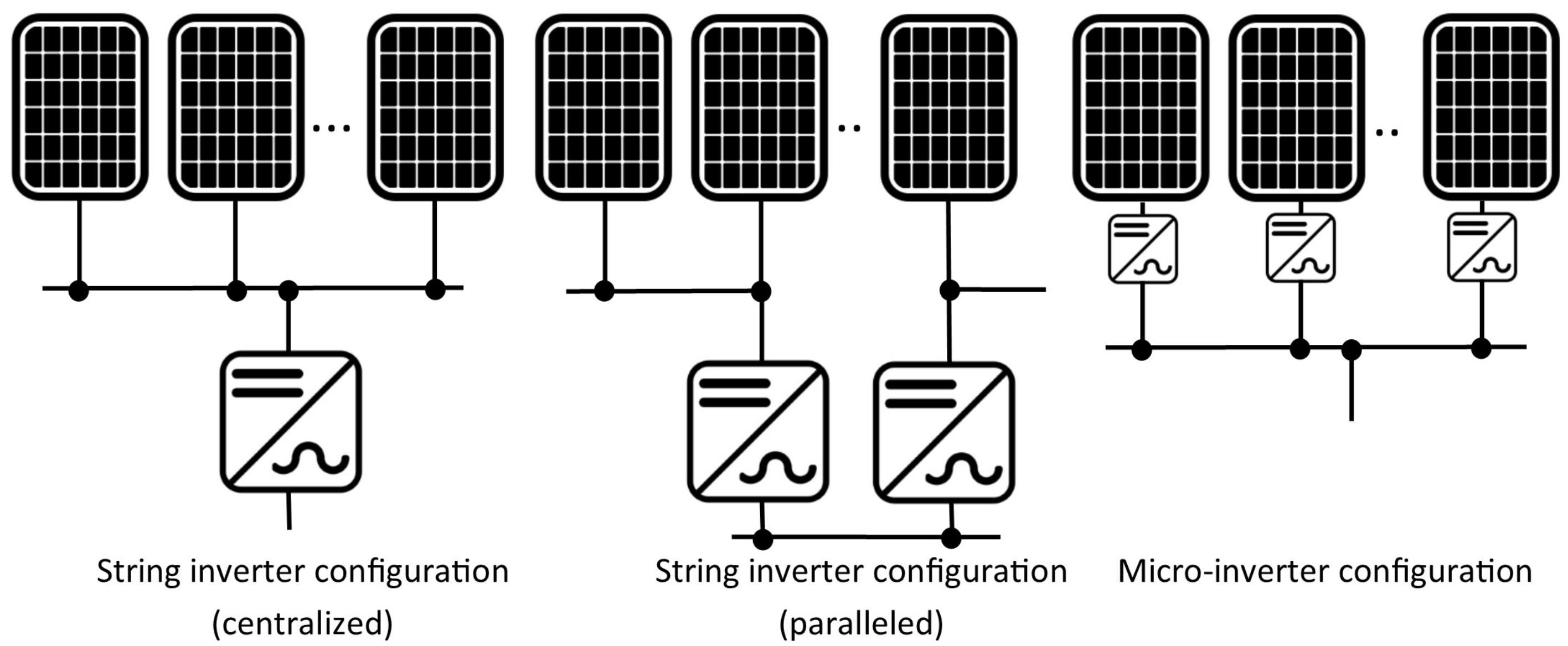
• We have defined PV systems that use Enphase [22], Enecsys [23], or Involar [24] inverters as the micro-inverter configuration. These brands are the dominant suppliers in the PV market with an inverter size below 500 W. For other systems which use an inverter size larger than 500 W and the number of inverters less than the number of panels, we imply they are of string-inverter configuration. The common inverter configurations are shown in Figure 1.

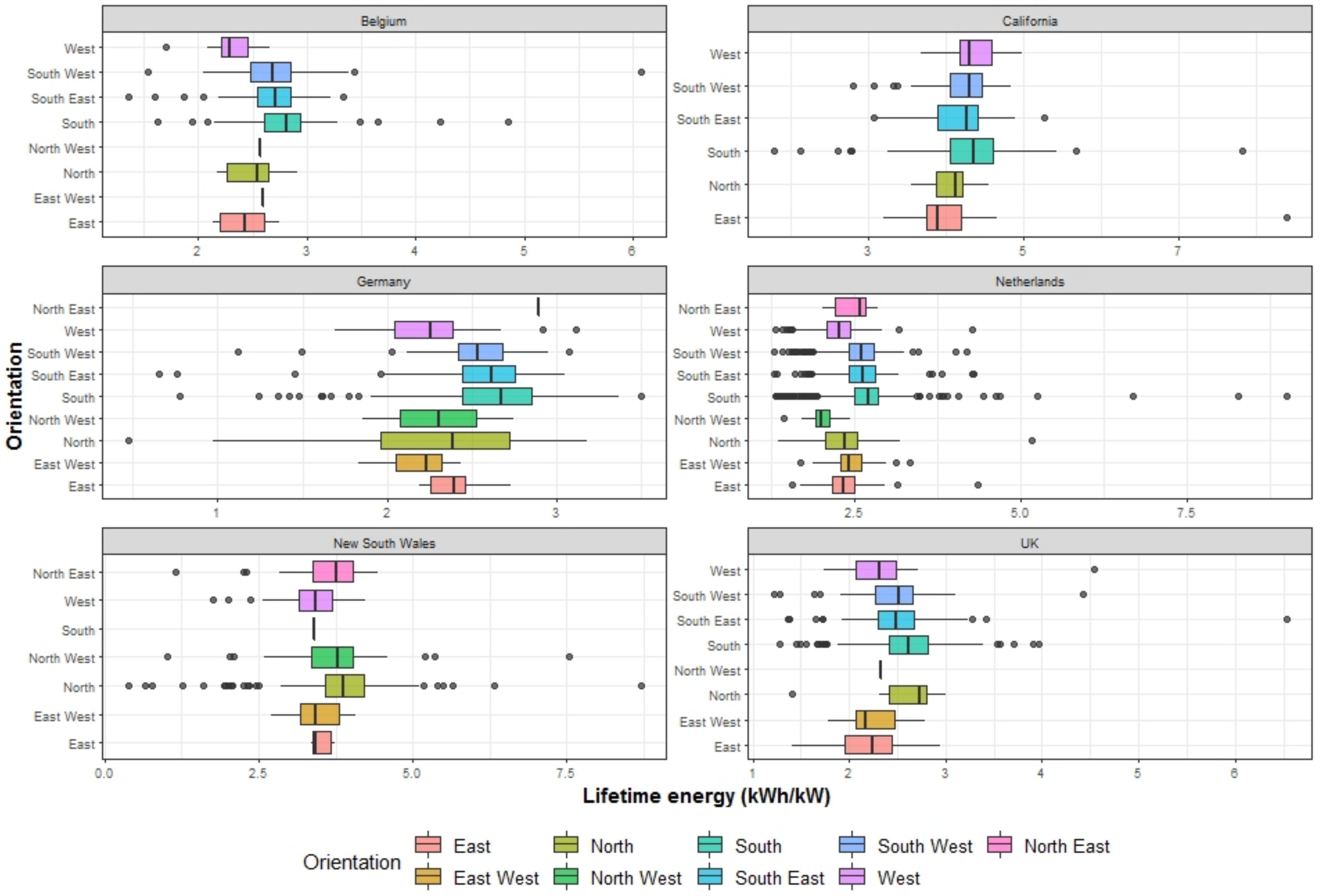
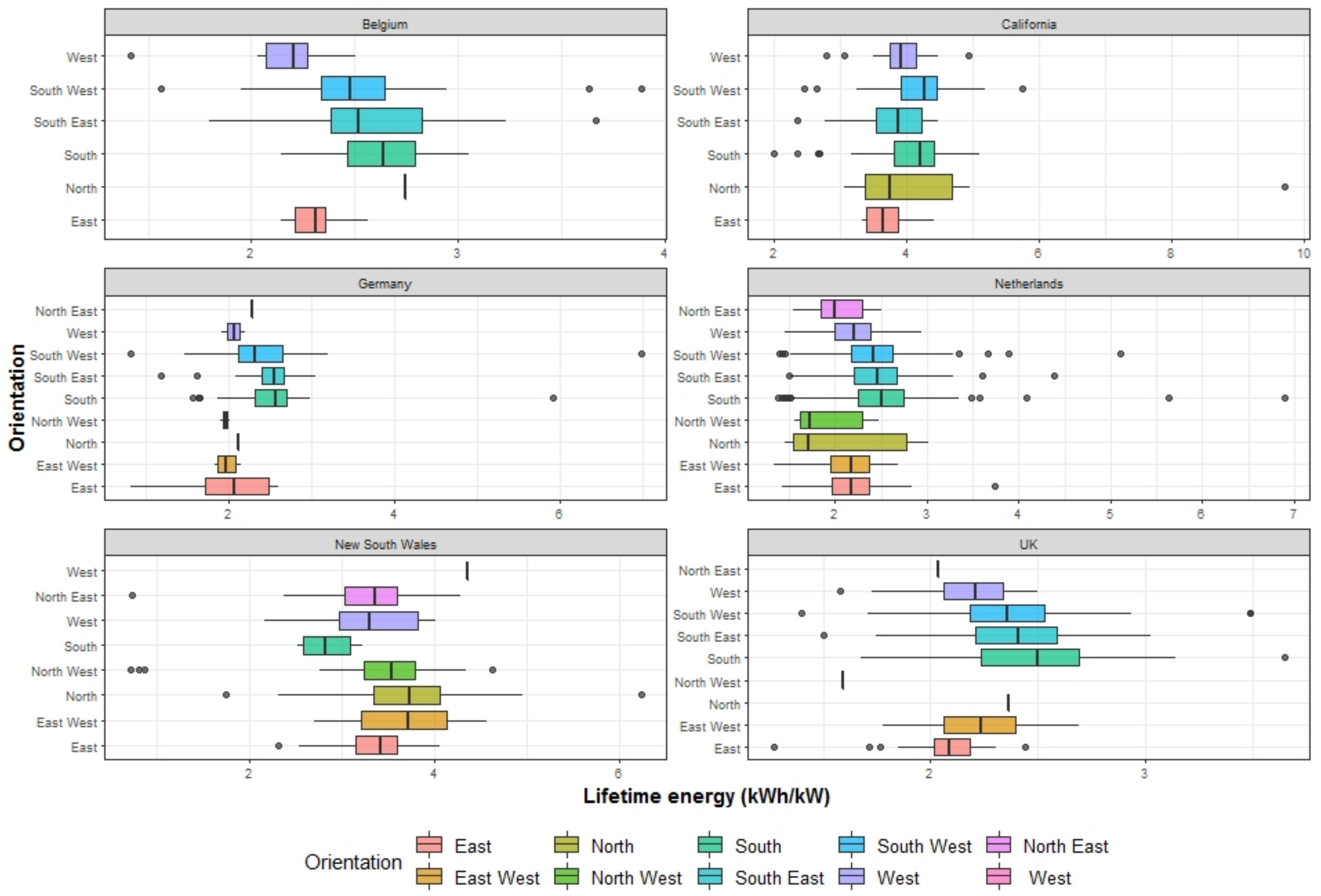
After applying the above criteria, we obtained the distribution of PV lifetime yield for the non-shading group in Figure 2 and for the shading group in Figure 3. The fact is that lifetime energy yield is also influenced by solar radiation, ambient temperature, wind speed and PV system aging. Unfortunately, these factors are not available in the pvoutput database. Therefore, we use the information about the panel orientation, panel tilt and PV location instead.

3. Applied Machine Learning Techniques

Machine learning techniques are based on the power of a computer to build and train models according to the input datasets. Its power is verified in many practical applications such as prediction or decision problems, rather than using static mathematical models. In this section, we represent two applied machine learning techniques—named the bootstrap technique and multiple linear regression—in order to evaluate the impacts of PV component and configuration on the lifetime energy yield.

3.1. Bootstrap Technique

The t-test (Student’s t-test) [25] is used to compare the mean values between two independent datasets when we investigate any difference. However, this test is only reliable when the dataset meets the prior assumptions of normal distribution, homogeneity in variance and absence of outliers. From the descriptions of lifetime energy yield in Figure 2 and Figure 3, these conditions are hardly satisfied by our datasets.

Bootstrap is one of the most widely known techniques in machine learning [26] and an alternative solution to the t-test. It improves the accuracy of the measurement when the number of datasets is not sufficient. Bootstrap is also useful for comparing groups with unequal sample sizes as seen in

Table 2. Summary of the rooftop PV systems in our study. The dataset was collected in August 2018.

Countries and Regions	Total PV Systems	Non-Shading Group				Shading Group
		Inverter Configuration		Inverter Brands		Inverter Configuration		Inverter Brands
		Micro	String	SMA	Others	Micro	String	SMA	Others
Belgium	504	10	360	273	97	3	131	98	36
California	462	120	153	27	246	91	98	18	171
Germany	513	12	364	286	90	12	125	108	29
Netherlands	3615	231	2068	779	1520	156	1160	408	908
New South Wales	540	40	290	121	209	32	178	74	136
United Kingdom	1095	58	626	35	649	36	375	17	394
Total	6729	471	3861	1521	2811	330	2067	723	1674

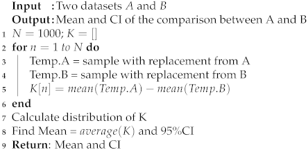
. In our study, we applied the bootstrap to answer the first two questions mentioned in Section 1. The detailed algorithm of our bootstrap is given in Algorithm 1.

Algorithm 1: Bootstrap technique to find the mean and $95\%$ confidence interval (CI) of a comparison.

The inverter is the most vulnerable component of a PV system [16]. It controls both DC input and AC output in order to obtain the maximum power. For this reason, we have chosen the inverter brand as the investigated PV component to check any significant difference in $Y_L$ among inverter brands. The SMAinverter [27] was chosen as the reference inverter to compare since this manufacturer has the highest volume of installed inverters in our PV dataset.

In order to measure any significant difference in $Y_L$ between micro-inverter and string inverter configurations, we have implied that all the PV systems that are installed with inverter of Enphase, Enecsys and Involar use the micro-inverter, others use the string-inverter. The comparison results are represented in Section 4.1 and Section 4.2, respectively.

3.2. Multiple Linear Regression Model

The multiple linear regression model was chosen to answer the last research question in Section 1 since this model is a useful approach to evaluating the contributions of many inputs to an output. We have limited our study to the main factors of PV design configuration and component—the number of solar panels, the rated power of panel, the number of inverters and the inverter power. These four inputs are the most important factors that a customer is recommended to identify at the initial step of their PV planning and design.

We assume that the lifetime energy yield $Y_L$ from a PV system can be represented by the multiple linear equation as Equation (2).

$$Y_L=\alpha +{\mathit{\beta }}^T\mathit{X}+ϵ$$

(2)

where $\alpha$ and ${\mathit{\beta }}^T=\left[\begin{array}{cccc}{\beta }_1& {\beta }_2& {\beta }_3& {\beta }_4\end{array}\right]$ are the regression coefficients. $ϵ$ is the residual (the error) from the regression model. $\mathit{X}$ is the matrix of input values as Equation (3).

$$\mathit{X}={\left[\begin{array}{cccc}{x}_1& x_2& x_3& x_4\end{array}\right]}^T$$

(3)

where $x_1$, $x_2$, $x_3$, and $x_4$ are the number of solar panels, the rated solar power, the number of inverters and the inverter power, respectively. From Equation (2), the residuals $ϵ$ are calculated as Equation (4).

$$ϵ=Y_L-(\alpha +{\mathit{\beta }}^T\mathit{X})=Y_L-{\widehat{Y}}_L$$

(4)

where ${\widehat{Y}}_L$ is the estimated lifetime energy yield from model.

In order to prove the multiple linear regression assumption, the residuals in Equation (4) are analyzed. According to the four assumptions in Reference [28], the residuals have to ensure the following conditions:

• The residuals $ϵ$ have a normal distribution;
• The mean equals to zero;
• The variance is constant.

It means that the distribution of residuals is as Equation (5).

$$ϵ\sim N(0,{\sigma }^2)$$

(5)

where the mean is zero and the variance of residuals is ${\sigma }^2=constant$.

To prove the normality of the residuals, we formulate the hypothesis test of normality as below:

• The null hypothesis ($H_0$): The residuals $ϵ$ are normally distributed. If the result of the test of significance, represented by the p value, is larger than $0.05$, normality can be assumed;
• The alternate hypothesis ($H_1$): The residuals $ϵ$ are not normally distributed. In this case, the p value is smaller than 0.05.

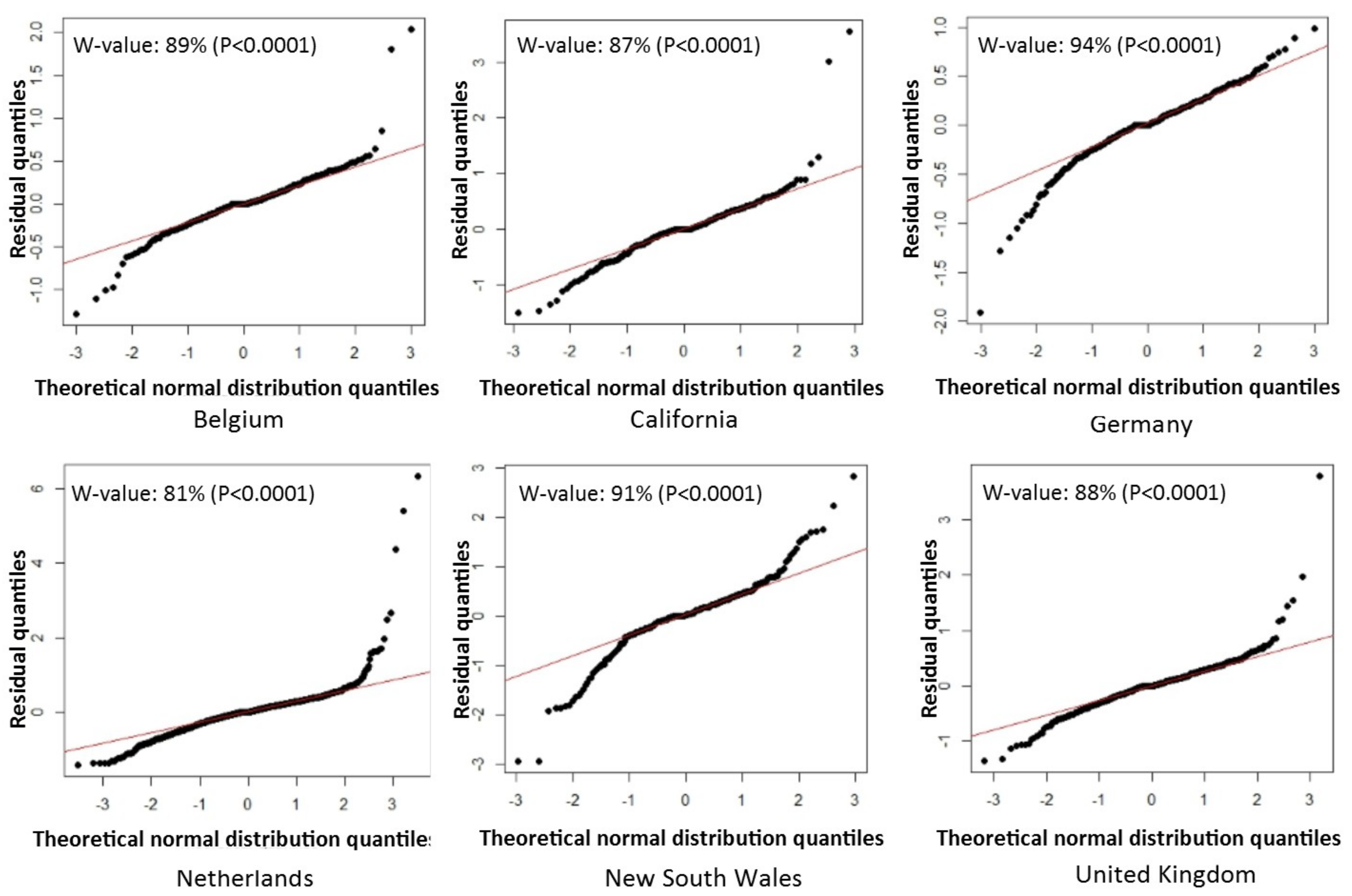
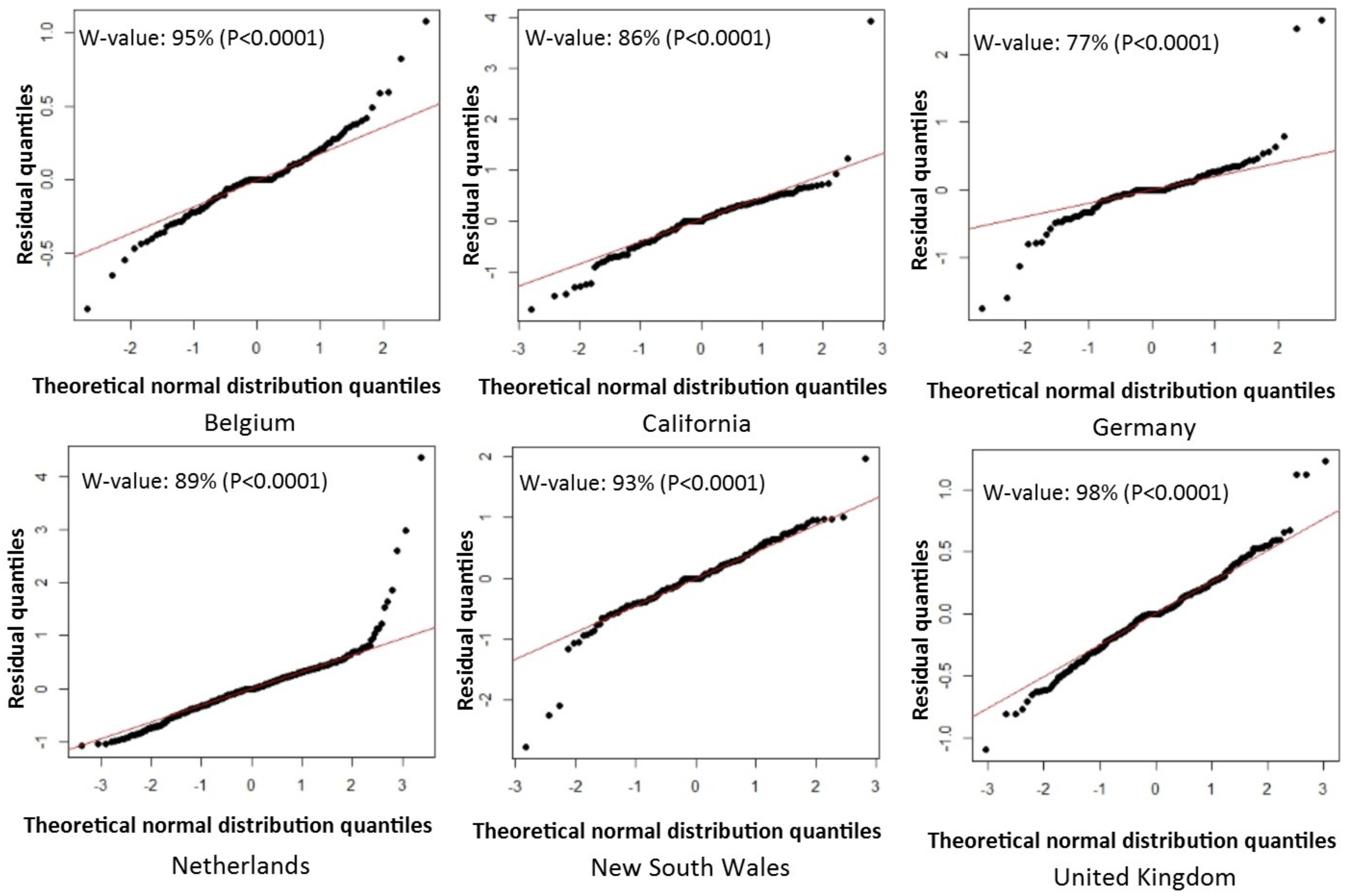
The Kolmogorov-Smirnov test [29] and Shapiro-Wilk’s W test [30] are common methods for testing normality. However, both tests are sensitive to outliers and are influenced by sample size. Hence, the test of normality should be used in conjunction with the normal quantile-quantile (Q-Q) plot. These normality plots of multiple linear regression models in Section 4.3 are shown in the Appendix A.

4. Performance Results and Discussion

The Algorithm 1 and multiple linear regression model were implemented using R programming version 3.4.0 [31] and the linear regression lm package [32]. All random processes used the same number of generators to ensure the reproducibility.

4.1. Impact of Inverter Brands

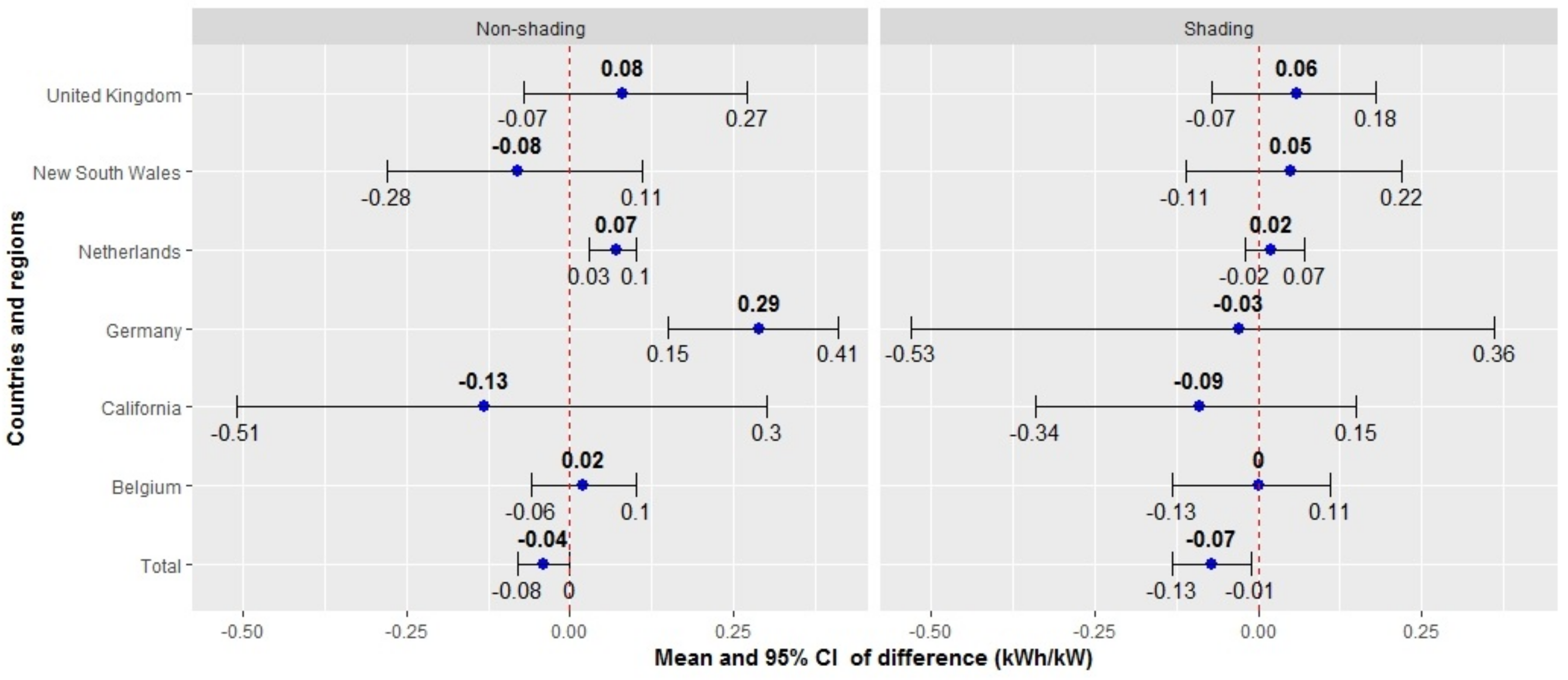
Figure 4 depicts the mean of difference and $95\%$ confidence interval (CI) of the mean in lifetime energy yield between systems that use an SMA inverter and systems that use other inverters throughout countries and regions. Under the non-shading condition, we found that the PV systems that use SMA inverters have higher $Y_L$ than the others only in the Netherlands and Germany. In these two countries, the $95\%$ CI ranges of the mean in Figure 4 do not cross zero value, hence the results are significantly different. For other countries and regions, it is not evident to conclude any significant difference since the CI ranges of mean cross zero value.

Under the shading condition, no significant difference in $Y_L$ in any country and region were found since all the $95\%$ CI ranges include zero values. This means that, compared to other inverter brands, the SMA inverter does not have any advantage. Finally, we have found that the type of inverter does not significantly affect the lifetime energy yield at the global scale because the $95\%$ CI ranges are from −0.08 (kWh/kW) to 0 (kWh/kW) in non-shading and from $-0.13$ (kWh/kW) to $-0.01$ (kWh/kW) in shading. However, these findings do not take into account the real working conditions of the inverter, for example the inverter is placed indoors or outdoors, the maximum power point tracking (MPPT) technique of the inverter.

4.2. Impact of Inverter Configurations

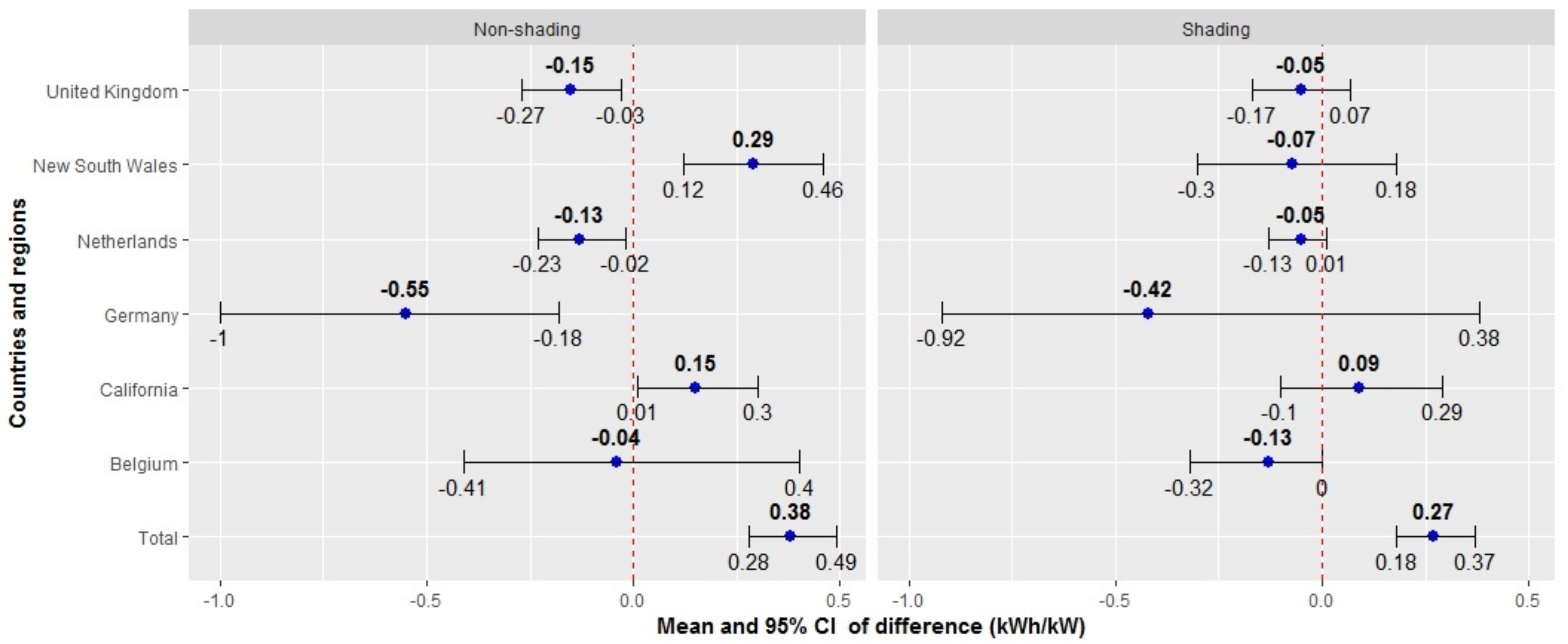
Figure 5 shows the mean of difference and $95\%$ confidence interval (CI) of the mean in lifetime energy yield between systems that use a micro-inverter configuration and systems that use a string inverter throughout countries and regions. Under non-shading condition, the PVs that use a micro-inverter produce a lower energy yield than the ones that use a string inverter in European countries. Meanwhile, in the subtropical climate regions (New South Wales) and Mediterranean-like climate regions (California) the PVs that use a micro-inverter configuration produce a higher lifetime energy than those that use a string inverter.

Under the shading condition, no significant differences in $Y_L$ were found since all the $95\%$ CI ranges include a zero value. This finding contrasts with previous results reported in the literature indicating that the micro-inverter configuration obtained a higher energy yield than other configurations. A possible reason explaining this contrast is that the efficiency of the micro-inverter has been affected by the temperature in outdoor conditions. Therefore, this leads to a lower energy yield than the string inverter, which is usually placed inside the home.

On the global scale, we found that the PVs that use a micro-inverter obtain a higher lifetime energy than those that use a string inverter under both conditions. This finding is also in good agreement with the previous studies in References [33,34]. However, this conclusion still needs more longitudinal studies with PV data from many countries and regions in order to obtain a stronger conclusion about the advantage in energy yield of PV systems using a micro-inverter configuration.

4.3. Contribution of PV Panel and Inverter Configurations

Table 3. The results of the multiple linear regression analysis of panel and inverter configurations.

Countries and Regions	Non-Shading Group				Shading Group
	Residual Standard Error	Degree of Freedom	R-Squared Value	Significance of Model (p Value)	Residual Standard Error	Degree of Freedom	R-Squared Value	Significance of Model (p Value)
Belgium	0.34	280	36%	0.0001	0.33	81	45%	0.15
California	0.58	208	31%	0.03	0.65	136	38%	0.015
Germany	0.37	275	43%	<0.0001	0.61	77	48%	0.18
Netherlands	0.43	2056	15%	<0.0001	0.40	1130	20%	0.0001
New South Wales	0.75	255	37%	<0.0001	0.65	141	37%	0.16
United Kingdom	0.40	573	18%	0.19	0.32	334	21%	0.15

demonstrates the results of the multiple linear regression models in Section 3.2 in both non-shading and shading conditions. Note that the lifetime energy $Y_L$ is the linear combination of the number of solar panels, the rated solar panel power, the number of inverters and the inverter power, respectively. The R-squared value measures the strength of contribution that comes from the inputs to the variance in the output on a convenient $0\%$ to $100\%$ scale. As we expected, the contributions of the above inputs to the variance of the output interpreted by R-squared values are below $50\%$ in either countries or regions. The highest contribution value is measured in Germany ($43\%$) in non-shading and ($48\%$) in shading. In addition, only the model of the United Kingdom is not statistically significant (p = 0.19) in the non-shading condition. However, under the shading condition, our regression model showed its limitation since only the models of California and the Netherlands are statistically significant ($p<0.05$).

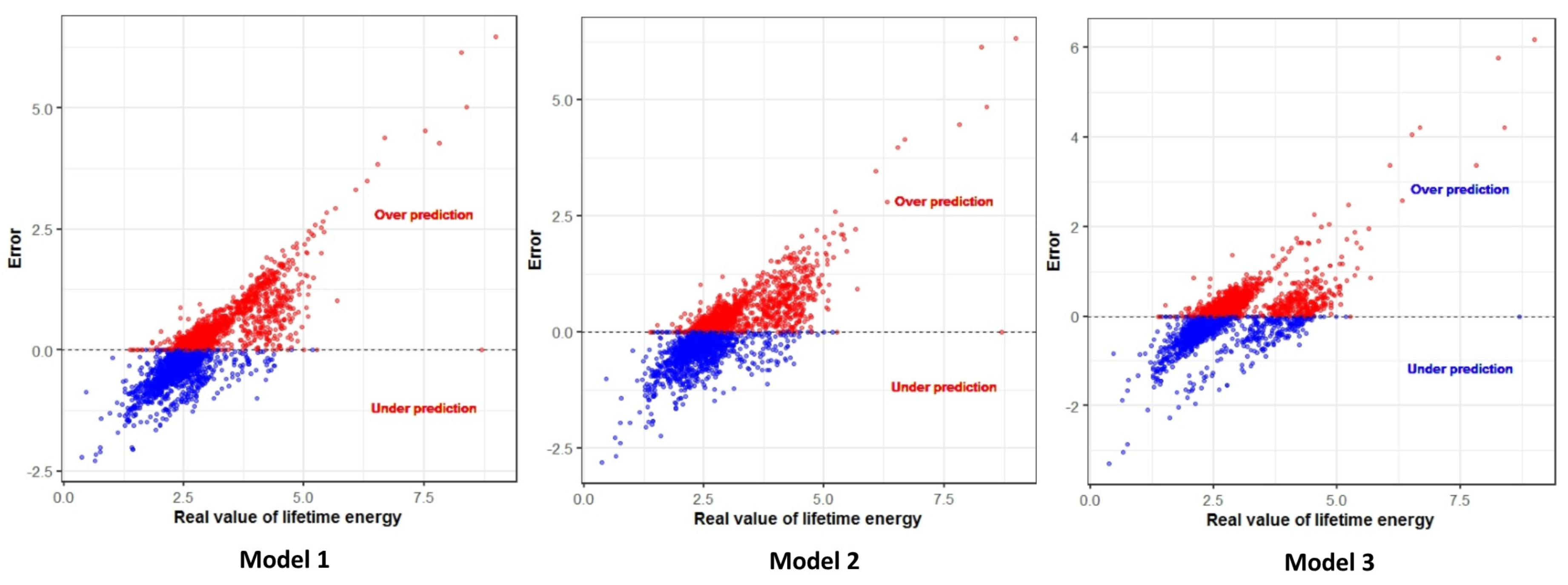
To further investigate the contribution of the geospatial inputs to the generated power yield ($Y_L$) in the non-shading condition of all PV datasets, the multiple linear regression model was extended in three scenarios as follows:

• Model 1: The inputs are the number of solar panels, the rated panel power, the number of inverters, and the inverter power;
• Model 2: The inputs are as in model 1, plus the panel orientation and panel tilt;
• Model 3: The inputs are as in model 2, plus the location of PV system.

The analysis results of the above three models are shown in

Table 4. The results of multiple linear regression analysis of all PV datasets.

	Residual Standard Error	Degree of Freedom	R-Squared Value	95% CI of R-Squared Value	Significance of Model (p Value)
Model 1	0.59	4029	31%	29–38%	<0.0001
Model 2	0.54	3631	43%	42–51%	<0.0001
Model 3	0.45	3626	61%	59–68%	<0.0001

. As expected, the contribution of the panel and inverter configuration in model 1 obtained the lowest R-squared value, with the mean $31\%$ ($95\%$ CI: 29–38%). Meanwhile, model 3 got the highest R-squared value with the mean $61\%$ ($95\%$ CI: 59–68%). Indeed, Figure 6 shows the trend of error between predicted energy yield and the real value when using three prediction models. Compared to models 2 and 3, model 1 with the given solar panel and inverter configurations tends to overpredict the energy yield from PV system. These results are not amazing because model 3 provides more details about the geospatial data of the PV station. Therefore, we strongly confirm the crucial role of geospatial data in any PV energy calculation model.

In order to prove the correctness of our regression model, the residual values were calculated as in Equation (4) and plotted the normality Q-Q plots in Figure A1, Figure A2 and Figure A3. These figures also show the results of the Shapiro-Wilk’s W normality tests. The W value indicates how close the residual distribution is to the normal distribution in terms of percentage and to the sensitivity in terms of p value of the Shapiro-Wilk’s test.

5. Conclusions

In this study, we investigated the lifetime energy yield of a rooftop PV system over the world, given technical details about the solar panel and inverter configurations by a measurable method based on machine learning. Our findings have shown that the contribution of both the panel configuration and the inverter configuration are still lower than the uncertain impacts of geospatial conditions. Furthermore, the PVs that use the micro-inverter configuration seem to obtain a higher energy yield than the PVs that use a string inverter. Lastly, the brand of inverter does not impact the generated energy of PV system significantly. In general, our work therefore might help a customer to choose a suitable PV investment plan, by considering the important role of geospatial conditions, rather than the high-price PV components.

Further research is required to verify the effects of geographic data such as solar radiation, temperature, or humidity on micro-inverter and string inverter configurations at the same location. We also plan to extend our study for other types of PV system configurations such as oversize panel or DC common bus.

References

- Varma, R.K.; Sanderson, G.; Walsh, K. Global PV incentive policies and recommendations for utilities. In Proceedings of the 2011 24th Canadian Conference on Electrical and Computer Engineering (CCECE), Niagara Falls, ON, Canada, 8–11 May 2011; pp. 001158–001163. [Google Scholar] [CrossRef]
- Aste, N.; Groppi, F.; del Pero, C. The first installation under the Italian PV rooftop programme: A performance analysis referred to five years of operation. In Proceedings of the 2007 International Conference on Clean Electrical Power, Capri, Italy, 21–23 May 2007; pp. 360–365. [Google Scholar] [CrossRef]
- Chaianong, A.; Tongsopit, S.; Bangviwat, A.; Menke, C. Bill saving analysis of rooftop PV customers and policy implications for Thailand. Renew. Energy 2019, 131, 422–434. [Google Scholar] [CrossRef]
- Bhandari, K.P.; Collier, J.M.; Ellingson, R.J.; Apul, D.S. Energy payback time (EPBT) and energy return on energy invested (EROI) of solar photovoltaic systems: A systematic review and meta-analysis. Renew. Sustain. Energy Rev. 2015, 47, 133–141. [Google Scholar] [CrossRef]
- Richter, M.; Tjengdrawira, C.; Vedde, J.; Jan, B.; Sicon, V.; Denmark, M.; Green, M.; Frearson, L.; Herteleer, B.; Stridh, B.; et al. Technical Assumptions Used in PV Financial Models Review of Current Practices and Recommendations; Technical Report; IEA International Energy Agency: Paris, France, 2017. [Google Scholar]
- Jäger-Waldau, A. Snapshot of photovoltaics—February 2019. Energies 2019, 12, 769. [Google Scholar] [CrossRef]
- Horowitz, K.A.W.; Fu, R.; Silverman, T.; Woodhouse, M.; Sun, X.; Alam, M.A. An Analysis of the Cost and Performance of Photovoltaic Systems as a Function of Module Area; Technical Report; National Renewable Energy Laboratory (NREL): Lakewood, CO, USA; U.S. Department of Energy: Washington, DC, USA, 2019.
- Perdue, M.; Gottschalg, R. Energy yields of small grid connected photovoltaic system: Effects of component reliability and maintenance. IET Renew. Power Gener. 2015, 9, 432–437. [Google Scholar] [CrossRef]
- Shaw-Williams, D.; Susilawati, C.; Walker, G. Value of residential investment in photovoltaics and batteries in networks: A techno-economic analysis. Energies 2018, 11, 1022. [Google Scholar] [CrossRef]
- Louwen, A.; Schropp, R.E.; van Sark, W.G.; Faaij, A.P. Geospatial analysis of the energy yield and environmental footprint of different photovoltaic module technologies. Sol. Energy 2017, 155, 1339–1353. [Google Scholar] [CrossRef]
- PVSITES Software. Available online: https://www.pvsites.eu/software/ (accessed on 15 January 2019).
- PVSYST Software. Available online: https://www.pvsyst.com/features/ (accessed on 15 January 2019).
- Google Project Sunroof. Available online: https://www.google.com/get/sunroofp=0 (accessed on 15 January 2019).
- PVWatts Calculator. Available online: https://pvwatts.nrel.gov/ (accessed on 15 January 2019).
- Suomalainen, K.; Wang, V.; Sharp, B. Rooftop solar potential based on LiDAR data: Bottom-up assessment at neighbourhood level. Renew. Energy 2017, 111, 463–475. [Google Scholar] [CrossRef]
- He, F.; Zhao, Z.; Yuan, L. Impact of inverter configuration on energy cost of grid-connected photovoltaic systems. Renew. Energy 2012, 41, 328–335. [Google Scholar] [CrossRef]
- Jiranantacharoen, P.; Bonprasert, K.; Le, N.T.; Benjapolakul, W. Energy efficiency evaluation of Thailand PV rooftop systems using machine learning techniques. In Proceedings of the 33rd International Technical Conference on Circuits/Systems, Computers and Communications (ITC-CSCC 2018), Bangkok, Thailand, 4–7 July 2018; pp. 1–4. [Google Scholar]
- Emziane, M.; Ali, M.A. Performance assessment of rooftop PV systems in Abu Dhabi. Energy Build. 2015, 108, 101–105. [Google Scholar] [CrossRef]
- Allouhi, A.; Saadani, R.; Kousksou, T.; Saidur, R.; Jamil, A.; Rahmoune, M. Grid-connected PV systems installed on institutional buildings: Technology comparison, energy analysis and economic performance. Energy Build. 2016, 130, 188–201. [Google Scholar] [CrossRef]
- PVOutput Dataset. Available online: https://pvoutput.org/ (accessed on 15 January 2019).
- Tjengdrawira, C.; Richter, M. Review and Gap Analyses of Technical Assumptions in PV Electricity Cost Report on Current Practices in How Technical Assumptions Are Accounted in PV Investment Cost Calculation; Technical Report; The Solar Bankability Consortium: Bozen, Italy, 2016. [Google Scholar]
- Enphase Microinverter. Available online: https://enphase.com/en-us/products-and-services/microinverters (accessed on 15 January 2019).
- Enecsys Micro Inverters. Available online: https://www.enecsysoutput.com/guide/installationGuideEnecsys.pdf (accessed on 15 January 2019).
- Involar Micro Inverters. Available online: https://www.eborx.com/download/en/involar/manual-micro.pdf (accessed on 15 January 2019).
- Haynes, W. Encyclopedia of Systems Biology; Springer: New York, NY, USA, 2013; pp. 2023–2025. [Google Scholar] [CrossRef]
- Jain, A.K.; Dubes, R.C.; Chen, C. Bootstrap techniques for error estimation. IEEE Trans. Pattern Anal. Mach. Intel. 1987, PAMI-9, 628–633. [Google Scholar] [CrossRef]
- SMA Solar Inverters. Available online: https://www.sma.de/en/products/solarinverters.html (accessed on 15 January 2019).
- Osborne, J.; Waters, E. Four assumptions of multiple regression that researchers should always test. Pract. Assesss Res. Eval. 2002, 8, 1–5. [Google Scholar]
- Wilcox, R. Kolmogorov–Smirnov test. In Encyclopedia of Biostatistics; John Wiley & Sons: Hoboken, NJ, USA, 2005. [Google Scholar] [CrossRef]
- Royston, P. An extension of Shapiro and Wilk’s W test for normality to large samples. Appl. Stat. 1982, 31, 115–124. [Google Scholar] [CrossRef]
- The R-Project for Statistical Computing. Available online: https://cran.r-project.org/bin/windows/base/ (accessed on 15 January 2019).
- Adams, M. lm.br: Linear Model with Breakpoint, R Package version 2.9.3; The R Foundation for Statistical Computing: Vienna, Austria, 2013. [Google Scholar]
- Famoso, F.; Lanzafame, R.; Maenza, S.; Scandura, P.F. Performance comparison between micro-inverter and string-inverter photovoltaic systems. Energy Procedia 2015, 81, 526–539. [Google Scholar] [CrossRef]
- Harb, S.; Kedia, M.; Zhang, H.; Balog, R.S. Microinverter and string inverter grid-connected photovoltaic system—A comprehensive study. In Proceedings of the 2013 IEEE 39th Photovoltaic Specialists Conference (PVSC), Tampa, FL, USA, 16–21 June 2013; pp. 2885–2890. [Google Scholar] [CrossRef]
© 2019 by the authors. Licensee MDPI, Basel, Switzerland. This article is an open access article distributed under the terms and conditions of the Creative Commons Attribution (CC BY) license (http://creativecommons.org/licenses/by/4.0/).