Abstract
The EU decarbonization strategy foresees deep cuts in CO2 in the transport sector. Investment in infrastructure, manufacturing of new technology vehicles and production of alternative fuels induce macroeconomic changes in activity and employment for both national and regional economies. The objective of the paper is to present a newly built macroeconomic-regional model (GEM-E3-R general equilibrium model for economy, energy and environment for regions) for assessing impacts of transport sector restructuring on regional economies of the entire EU, segmented following NUTS-3 (nomenclature of territorial units of statistics). The model combines general economic equilibrium theory with location choice and New Economic Geography and implements a dynamic, fully endogenous agglomeration-dispersion mechanism for people and industries coupled with a gravity model for bilateral interregional flows. A novelty of the model is a two-layers structure: (i) the country-wide layer formulated as a global multi-sector, multi-country and multi-period computable general equilibrium (CGE) model; and (ii) the regional economy layer, which simulates impacts on regional economies, while considering country-wide economic trends as boundary conditions. The paper presents a use of the model in the assessment of regional economic effects of electrification of car mobility in Europe and wide use of domestically produced advanced biofuels.
1. Introduction
Carbon dioxide emitted in the EU transport sector accounted for 27% of total EU-wide greenhouse gas (GHG) emissions in 2016, according to Reference [1]. Transport sector emissions have increased by 26% since 1990. Transport-related expenditures represent 12–15% of total expenditures by firms and households, while the supply of transport services employs 10 million persons directly and an additional 11 million indirectly, according to Reference [2]. Decarbonizing transport is essential for achieving the EU low carbon emission targets. The European Commission’s climate policy regarding the transport sector, as described in the White Paper on transport in 2011, see Reference [3], and re-confirmed in the 2018 “A Clean Planet for All” long-term strategy, see Reference [4], has set ambitious targets for reducing transport-related emissions. The strategy envisages ways to decarbonize the vehicle fleet, mainly through electrification, the use of biofuels and carbon-free alternative fuels. The policy measures already adopted include the CO2 car standards and the forthcoming energy efficiency standards, while a multitude of transport infrastructure developments aim at facilitating higher efficiency via transport modal shifts.
The transport sector is particularly inflexible in emission abatement because it depends on fossil oil products and the alternatives are not yet mature. Transport sector restructuring towards low carbon emissions requires a complete change in the technology of transport fleet, development of infrastructure for electricity, and the production of alternative fuels, such as biofuels, hydrogen and carbon-neutral synthetic hydrocarbons. The changes imply a considerable increase in investment in the transport sector both for the fleet and infrastructure. In addition, the replacement of imported fossil oil products by domestically produced fuels implies a significant rise in domestic economic activity for electricity, biofuels, hydrogen, and synthetic fuels.
Consequently, transport restructuring towards low carbon emissions will convey multifaced impacts on the economy, both at the country and regional levels. We expect that the changes will act in favor of domestic production activity and employment but will have unequal impacts on regions. The changes may entail increased transport service costs, at least in the early stages of the transition, mainly before new technologies and alternative fuels fully attain their learning potential. An increase in transport costs drives the prices of goods and services upwards and causes crowding out effects that affect the economy negatively.
The economic effects are not uniformly distributed among regions. The regional distributional differences are attributed to local specificities regarding resource endowment, as well as human, environmental, and infrastructure features of regions. Agglomeration and dispersion forces, which differ by region, explain the different development paces to be experienced by the regions due to the transport sector restructuring. The regional features, such as industrial facilitation, skill availability, accessibility of the region, and several other factors, acting positively to attract activity are termed amenities and those acting negatively dis-amenities (e.g., pollution, congestion, isolation).
The focus of the paper is the modelling of regional distributional effects stemming from the rising economic activities due to the restructuring of the transport sector. Regional effects derive from the location of physical and human capital, which depend on regional features and policies, which in turn accumulate evolve dynamically. The model presented in this paper covers only the economic impacts and does not cover the engineering and economic features of transport sector restructuring fully, as transport sector models do in detail. The PRIMES-TREMOVE model [5], operated in our E3MLab research group, is preparing the details of decarbonization scenarios in the transport sector, which form the inputs to the economic model presented in this paper. Therefore, we did not expand on transport sector issues in this paper, but only on economic and regional effects of a given transport restructuring scenario. However, the economic model can handle any kind of transport sector restructuring assumptions.
The changes implied by transport sector decarbonization affect several industrial sectors directly (e.g., automotive industries, electric batteries, biofuels production, electricity production) and all other sectors indirectly, notably via the change in the costs of transport services. The changes also influence the allocation of family budgets to consumption of durable and non-durable goods. To capture the sectoral effects adequately, we developed a multi-sector and multi-country model and a multi-regional economic model. Due to the importance of foreign trade for economic growth, the multi-country model covers the global economy. We applied a computable general equilibrium methodology because of its consistency in simulating structural changes in the long-term. The main novelty of the model presented in this paper is the GEM-E3-R model, which is a fully-fledged macroeconomic and regional model that simulates a two-layer economic equilibrium of the national and subnational economies dynamically. The model calculates the effects on production, employment, intra- and international trade flows and GDP, while it calculates the location choices of agents (households and firms) and the inter-regional flows endogenously. The country-level model is a computable general equilibrium model with global coverage and the regional-level model implements a segmentation of countries in regions according to NUTS-3. The model ensures full equilibrium conditions in the markets for commodities, services, labour and capital.
The sub-country layer of the model downscales the country-wide economic trends into NUTS-3 regions for the EU28 member states. Sectoral activity and employment in the regions depend on the location of primary production factors, such as labour and capital, across the regions. Migration of the production factors, driven by regional features, changes labour and capital endowment of the regions and further influences activity and employment. The locational changes are meant to depend on an attractiveness indicator evaluated by region as an aggregation of the amenities and dis-amenities of the regions, which further depended on accumulation of state-variables and resources via stock-flow relationships. As the NUTS-3 regions are relatively small, the model includes commuting among regions endogenously. Also, the model paid attention to model inter-regional flows of goods and services endogenously, including transit flows.
The two-layer approach has advantages compared to alternative approaches that are common in the literature and model the regions directly. The two-layer approach ensures stability of regional projections because the simulated changes in regional economies use country-wide economic trends as boundary conditions. Also, the two-layers approach eases the computational complexity because it solves the models in a modular way via iterations.
The model uses non-linear functions to model the amenities by region and the agglomeration and dispersion effects. The stock-flow relations are also non-linear, to represent economies and dis-economies to scale, and act importantly as controls of regional specialization. In this manner, the model can simulate possible persistence of economic divergence among the regions, also within the same country, while avoiding irrational agglomeration.
The paper is structured as follows: Section 2 provides a literature review of spatial economic modelling and transport impact assessment studies, as well as an overview of the GEM-E3-R model; Section 3 includes the results of an illustrative simulation which highlights the main properties of the model; and Section 4 provides details on future improvements of the model and further research.
2. Spatial General Equilibrium Modelling
2.1. Literature Survey
The role of transport in international trade, the impacts on the environment, as well as transport as a driver of agglomeration have been thoroughly investigated in the past with the use of applied economic models, as in References [6,7]. It is only in the last decade that the role of transport in a decarbonizing context has emerged in the modelling literature. Models with a spatial dimension are necessary to assess the effects of transport policies and infrastructure developments adequately, as transportation depends on spatial networks. For this reason, a large part of the literature has focused on the assessment of transport infrastructure; References [8,9] and more recently Reference [10] provide reviews, whereas Reference [11] explores the relationship between transport costs and spatial agglomeration.
Spatial Computable General Equilibrium (SCGE) models constitute a distinct category among various models because they combine spatial and macroeconomic modelling. The spatial economic models can be broadly classified into the following categories (according to Reference [12]): (i) top-down models, in which the general equilibrium model is identical to a country-wide model and the results are simply regionalized according to a predefined and usually constant disaggregation rule; (ii) bottom-up models, in which the general equilibrium methodology is applied directly at the regional level (see References [13,14,15,16,17,18,19]); and (iii) single region models. To our knowledge, two-layer models (i.e., national and regional combined) are absent in the literature.
A survey of bottom-up SCGE models is provided by Reference [20] using a classification of approaches based on the following features: (i) formulation of labour mobility; (ii) ways of handling discrepancies between investment and savings at a regional level; (iii) differentiation of locations of employment and expenditures; and (iv) consistency between central and regional public finances.
Another classification of spatial economic modelling uses the following criteria, according to Reference [21]: (i) the theoretical basis of the model (general equilibrium theory versus location theory and new economic geography); (ii) the spatial linkages, given that poor spatial resolution diminishes the accuracy of modelling spatial economic effects; (iii) the dynamics of the model and the type of foresight implemented in the model; and (iv) the labour market specification.
The challenges of spatial general equilibrium modelling for transport impact assessment are described briefly as follows, according to Reference [22]: (i) interfacing problems between the macroeconomic and transport models; ii) the modelling of the influence of transport costs on sectoral production; (iii) the aggregation of micro-level data for product varieties in the macroeconomic model; and (iv) the problem of irrational agglomeration effects for regional economic activities.
In our model design, we addressed the interfacing problem by fully integrating transport modelling in the macroeconomic model. However, the transport model was more aggregated and had much lower resolution than fully-fledged transport models. We took care to account for transport cost in production and trade in all sectors. However, the sectoral segmentation, although more detailed than in other known models, is still aggregated with regard to micro-data for product varieties, due to data limitations. Regarding the issue of irrational agglomeration, we believe that our two-layer modelling approach improves the robustness of agglomeration projections because country-wide developments restrict the evolution of regional features and, thus, avoid unbounded agglomeration or dispersion.
Top-down models were initially based on the LMPST approach (acronym from the names of the authors Leontief, Morgan, Polenske, Simpson, Tower, also called “top-down regional extension”) as presented in Reference [23]. The authors apply a regionalisation of country-wide production by sector, but both the regional split shares and the interregional flows are constant in this approach. The disadvantages of this approach, according to Reference [14], are briefly as follows: (i) confinement of capital mobility within a single country level; (ii) absence of price differentiation between regions; and (iii) absence of endogenous adjustment of industrial location across the regions. To overcome drawbacks, other regional models have focused on introducing a flexible rather than fixed regional split of industries, as in References [24,25], and some of them have applied gravity-based formulations to derive the split, such as Reference [26].
To model industrial location across the regions, a vast body of literature employs the concept of attractiveness of a region approximated through a function that aggregates the performance of a region in terms of several criteria (features). Changes in the economy may modify the values of the regional features, hence, the value of the attractiveness indicator, thus driving changes in location choices of households and firms. The idea of using an aggregation function to measure the attractiveness of a region as a determinant of location choices draws on, among others, References [27,28,29,30,31,32,33]. The valuation of regional amenities is the same concept as evaluation of performance on criteria–features of a region. The aggregation of the amenities, as in Reference [28], as an attractiveness index, enters the household’s utility function, which further drives the location choice of residence. Similarly, the valuation of amenities drives migration flows, as in Reference [32]. The concept of amenities has its origins in literature dealing with quality of life indexes, and, in particular, the approaches that introduce amenities to explain regional disparities in wages, as in References [29,34,35]. The decision criteria, which enter the utility function as arguments, are termed “amenities” when the attractiveness index (AI) is positively influenced, and “dis-amenities” when the AI is negatively influenced, as in References [36,37]. The AI influences the decision making of households and firms through changes in the utility or the production functions, respectively. The definition and measurement of amenities can include qualitative factors (i.e., other than income for households and cost of primary factors of production) which are important for the choice of location by individuals and firms. Several similar approaches can be found in the literature on regional economics, see References [28,29,30,31,32,33,34,35,36,37,38,39,40,41,42,43].
The early SCGE models were static in nature and were used mainly for comparative static policy exercises. The introduction of the time dimension was firstly concerned with the stock-flow dynamics of capital and labour, see References [44,45]; for a detailed discussion on the dynamics of spatial CGE models see Reference [46]. However, there is lack of literature regarding the introduction of stock-flow dynamics for the valuation of amenities and dis-amenities and their effects on the attractiveness index. Agglomeration driven by attractiveness of a region may imply accumulation of activity, labour, capital and population accompanied by economies to scale, but also accumulation in the use of resources, or degradation of environmental quality, accompanied by or dis-economies to scale. Both would further drive amenity valuation upwards or downwards. Thus, a state variable, measured as a stock rather than a flow—for example, status of the environment—exerts a feedback effect on amenities, hence, on the attractiveness of regions. The stock-flow relationship exhibits economies or diseconomies to scale. The introduction of such stock-flow relationships is important to allow the model to find a balance in the location choices across the regions, instead of increasing location preferences for a region in an unlimited way, which is a serious drawback in some of the models in the literature. In addition, the regional layer of the GEM-E3-R model formulates amenity valuation, hence, attractiveness functions, using stock-flow relationships in a dynamic manner. This is a novelty of the model, compared to the existing literature.
We built on the standard version of the GEM-E3 model, see Reference [47], to develop the regional economic equilibrium model. The standard GEM-E3 model was extended to incorporate a detailed formulation of transport-related decisions of households and transport service supply sectors, following the modelling details provided in Reference [48]. The same model was also extended to formulate, in detail, the energy sector. The aim of the extended model is to study the economic impacts of decarbonization policies, similarly to References [49,50,51].
Computable general equilibrium (CGE) models are a distinct category of macroeconomic models, having neo-Keynesian or econometric macroeconomic models as main rivals. The CGE models inherited the Leontief inter-industrial input–output approach, see Reference [23], but formulate flexible functional forms for production and consumption functions instead of fixed technical coefficients. The CGE models rely on the Arrow–Debreu economic equilibrium theory and reproduce a price-driven simultaneous equilibrium of all markets for commodities and factors depending on microeconomic optimisation of utility and profit by consumers and producers, respectively. The Walras law, built into the model, ensures the balance of all flows of money (in constant terms), justifying a qualification of the model as general economic equilibrium, rather than partial equilibrium that characterise energy and transport sector models.
The CGE models have the advantage of accounting for all the interactions in an economy while handling demand and supply balancing consistently, regarding both volume and monetary transactions. The CGE model calculates the final status of the economy after reacting to an exogenous change and readjusting until reaching a new equilibrium. The consistency feature combined with the structural representation of microeconomic behaviours constitute the main advantages of the CGE modelling approach and justify the use of the model in impact assessment mainly regarding structural changes in the medium and long term. A CGE model ignores the way the economy transits through dis-equilibrium stages until reaching the general equilibrium. Bottlenecks, imperfections, and deficiencies, which may jeopardize the achievement of equilibrium, are outside the scope of a CGE model. Similarly, unused production capacities, deficits in financing, and persisting unemployment are not explicit in a CGE model.
In contrast, neo-Keynesian models are strong in representing dis-equilibria, unused capacities, debts, and unemployment, and, thus, have a short-term focus. The CGE models rely on a static dataset, albeit with numerous parameters that are difficult to estimate. The econometric models use time series to estimate the model parameters and include dynamic formulations aimed at capturing dynamic adjustments and often business cycles. However, the econometric and neo-Keynesian models are not fully consistent regarding the microeconomic foundation of decisions by consumers and producers. They also lack constraints to balance the uses and resources in the economy, either instantaneously or following a gradual long-term adjustment, as the CGE models are doing.
For these reasons, the CGE approach is clearly advisable (also supported by Reference [52]) for assessing the macroeconomic impacts of transport and energy sector restructuring, investment and relevant policy measures, such as CO2 car standards and taxation.
The review in Reference [52] concludes that the following features of the CGE approach are important for achieving high quality in the modelling of the interplay between transport and the economy: (i) the resolution of the model regarding the transport network; (ii) the representation of transport modal choices; (iii) the dynamic aspects of the model; and (iv) the flexibility of the functional forms. High resolution in the representation of transport networks and the choice of transport modes are difficult to incorporate in a full-scale CGE regional model due to the high computational complexity. We believe that our model has sufficiently high resolution for a CGE model, however, much less than transport-dedicated models. Our model formulates the dynamics of investment, although not with prefect foresight due again to computational limitations. However, it employs fully flexible functional forms both for consumption and production.
2.2. Overview of the GEM-E3-R Model
2.2.1. The Country-Wide Economic Equilibrium Model
The country-wide layer (CL) is a multi-sectoral, multi-regional, dynamic general equilibrium model (CGE). Compared to a standard economic equilibrium model, the CL introduces formulations to represent the location choices, the inter-regional flows, and the regional economic production and consumption subject to the country-wide (and EU-wide) economic equilibrium.
The CL model is a simultaneous system of mixed-complementarity conditions, derived as Kuhn–Tucker conditions of microeconomic optimization of the agents (i.e., suppliers and consumers) and equilibrium conditions covering all markets for commodities and primary production factors (i.e., labour and capital) simultaneously. The dual variables of the equilibrium conditions determine the prices of commodities and primary production factors. A balance equation acting as a closure of money flows represents the Walras law and, consequently, the model determines all except one of the prices (or a price index), which is the numeraire. The equilibrium runs over time dynamically based on stock-flow relations for capital, labour, and other variables. The optimisation of agents’ behaviours includes foresight, which adjusts over time myopically in the standard model version.
The agents are households, firms, and the government. They are specific to each country. Households derive demand for commodities and supply of labour from utility maximization under a budget constraint, which depends on revenues from wage salaries, dividends, and social benefits. Consumption splits in categories of utility drivers (e.g., food, health, entertainment, housing transport services) and form an aggregated utility function. The model formulates an optimization problem which maximizes utility subject to income to derive consumption by product and supply of labour (in other terms, participation in the labour market). The population and labour forces evolve in the future exogenously, based on assumed demographic factors. Labour mobility across regions is endogenous, depending on wage differentials and the regional attractiveness calculated for each region endogenously. At the country level, labour is mobile only among sectors within national borders.
Firms produce a single representative output by sector of activity. The outputs are differentiated depending on sector and country origin. The outputs are inputs to other sectors used together with primary production factors (labour and capital) to produce the output by sector of activity. Production functions aggregate the inputs to represent the possibility frontiers of production technologies. The production possibilities evolve over time driven by exogenous productivity factors. The model formulates an optimization problem by sector to represent the choice of the production factor mix as a result of minimization of total production cost, assuming price-taking for all inputs, subject to the production technology possibility frontier. Within a year, capital stock acts as a restriction of the volume of production by sector. The model includes investment functions to project the increase or decrease in capital stock over time. The investment functions depend on the rate of return of existing capital stock, derived from the static equilibrium, and a foresight of the likely evolution of demand for the sector’s output in the future. The implementation of investment employs fixed proportions of goods and services, such equipment goods, construction, and several types of services, which further constitute part of the demand for goods and services in the economy.
The commodities, being distinct by sector and country of origin, are non-perfect substitutes for each other in the formulation of commodity trading, and in all choices for consumption or production mix. The model provides the possibility to specify some commodities as non-tradeable. Furthermore, the model assumes that all markets of commodities and primary production factors operate under perfect competition conditions, which imply that prices derive from marginal costs and all agents are price takers.
The government acts as a final consumer of commodities for public consumption and investment. The model includes the non-market services sector to formulate production, choice of inputs, and investment of the public sector. The model included a variety of fiscal policy instruments, which aim to collect revenues to finance public investment (determined exogenously) and subsidies to firms or households, along with policy instruments for social benefits, social security, and transfer payments.
Labour, distinguishing a few typical skills, is fully endogenous regarding both demand and supply. Demand for labour skills derives from cost optimization of production by sector of activity. A Phillips curve, depending on labour force availability and unemployment, determines the relationship between the real wage rate and the labour market unemployment equilibrium by type of skill. The Philips curve represents frictions in the labour market due to the trade unions’ market power and other imperfections, such as mismatches in skill demand and supply. Thus, the curve supports a shift of labour supply function driving equilibrium unemployment, see Reference [53], which is higher than natural unemployment. The skill types are distinguished in the model only for the purpose of capturing wage differentials and productivity differences.
The CL model covers the global economy. The country resolution distinguishes all European countries individually, as well as major neighbouring countries (Table 1). The model distinguishes the G20 countries individually and divides the rest of the world into regions by grouping together the respective countries. The CL model segments the economy into 37 distinct sectors of activity, hence, 37 distinct goods and services for each country or group of countries.

Table 1.
Geographical coverage of the GEM-E3-R country layer (CL).
The segmentation of industrial sectors (Table 2) is appropriate for capturing the changes implied by transport decarbonization and electrification. For this purpose, the model distinguishes between electricity generation, electricity networks, and the fuelling sectors, including biofuels, and between car manufacturing and electric goods industries. The regional dataset specifies different regional endowments in the type and intensity of renewable resources, as some regions having high solar potential differ from those having high wind potential and those having high biomass feedstock production possibilities.
Table 2.
Sectoral coverage of the GEM-E3-R model.
The database of the model uses statistics from Eurostat (National Accounts, Public Finance, Input-Output tables, Labour statistics), WIOD (World Input-Output Table) and GTAP (Global Trade Analysis Project). A special routine performs model calibration, that is calculation of scale parameters of production and consumption functions to allow the model reproducing the base year statistics exactly. The model projects the entire structure of production, consumption and market equilibrium for all sectors and countries listed in Table 1 and Table 2.
2.2.2. Overview of Functional Forms Used in the Model
The production functions in the model represent nested choices of the production factor mix. The structure of the nesting (Figure 1), often called a nested scheme, is important for the magnitude of substitution or complementarity among the production factors. At each level of the nest, a single Allen substitution elasticity applies, but the values of elasticities differ across the nesting levels. In all levels, the functions aggregating the respective production factors followed the constant elasticity of substitution (CES) algebraic form, which involves scale parameters and an elasticity of substitution. The scale parameters are determined during calibration using the value shares of production inputs. Using dynamic calibration techniques, we vary the scale parameters over time, in particular for transport and energy choices, to make restructuring options possible, for example, regarding alternative fuels and electric vehicles. The same techniques are used to link the detailed transport or energy models to the economic model, so as to make the latter able to mimic the restructuring projections of the detailed models. In this manner, the production functions can produce input mixes like the fuel and technology mix suggested by transport and energy models in the context of decarbonization scenarios. We use this technique to link the general equilibrium model with projections using the PRIMES-TREMOVE models, which also operate in the E3MLab laboratory. In this manner, we introduce the transport and energy sector restructuring projections, calculated in dedicated models, in the economic and regional models to assess economic impacts adequately.
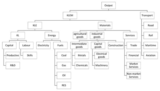
Figure 1.
Schematic representation of the GEM-E3-R nesting schemes for industrial sectors.
The production model solves for cost minimization to determine the input mix. Assuming constant returns to scale, the indirect minimum cost function separates the unit cost function from the volume of output. We thus apply the Shephard’s lemma to derive the optimum quantities of production inputs per unit of output volume. The typical formulation for a sector i producing at unit cost c using as an input priced at is as follows ( and are scale and elasticity of substitution parameters, respectively, whereas and are productivity factors):
The j index in the above formulation spans the production inputs. This index spans all goods and services with a distinction by country of origin. The product varieties are not perfect substitutes for each other, following the well-known Armington assumption, as in Reference [54].
The cost of using labour and capital in production depends, respectively, on wage rates (w) and the unit capital cost (r), both derived as equilibrium prices of the respective markets. Exogenously determined tax rates and social security contribution rates also affect the costs of primary production factors.
The investment functions are specified by sector of activity and determine the evolution of the stock of capital in the future. Within the static equilibrium the stock of capital by sector is given, acting as a constraint on potential output. The investment behaviour depends on anticipation of profitability by sector in the future, depicted by the endogenously determined rate of return on capital, the anticipation of future demand for the output of the sector, the cost of building new capital, and the rental cost of capital. The latter depends on interest rates derived in the model from the equilibrium of capital markets in an aim to represent how financial conditions influence profitability and thus investment. The formulations allow for capital mobility, but the allocation of capital to sectors and countries depends on assumptions that may differentiate interest rates and policy options obstructing or facilitating capital mobility. The model uses an investment matrix with fixed technical coefficients to transform investment by sector into demand for goods and services that implement the investment.
The model treats public investment in infrastructure, also in the transport sector, as exogenous. The implementation of investment in infrastructure transforms into demand for goods and services via an investment matrix, as for all other investment. Also, the accumulation of transport infrastructure investment, thus the increase in physical capital, induces positive productivity growth effects. The capital stock driving productivity changes is a mechanism that has rarely been seen in the literature of economic modelling. The aim is to capture the productivity effects of transport infrastructure, for example, the reduction in travelling times and the ensuing increase in productivity of labour and capital. The magnitude of the effects on productivity is specified exogenously, based on information collected from a vast literature of econometric estimation of productivity trends by sector in developed countries. Public investment also requires financing, which adds to the demand for funding in the economy and may increase the scarcity of capital, thus inducing an increase in interest rates. The model applies options to delimit the broadness of capital markets, as scarcity can be different when capital markets clear in the entire EU or on a country-by-country basis. The current version of the model does not allow for financial disequilibrium within the static equilibrium; thus, savings and investment must be balanced every year. This is a restrictive assumption as it cannot capture the mechanism of raising public investment in infrastructure expecting long-term repayment from accumulation of savings enabled by derived productivity growth. The static balancing implies that the rise of interest rates may obstruct public investment in case the funding affects capital scarcity. We plan to revise this assumption in future versions of the model.
The model formulates a representative household by country or region for the determination of consumption in durable and non-durable goods, together with savings and labour supply, as a result of intertemporal utility maximization subject to revenue constraint, which also depends on labour supply indirectly. As the simulation over time is sequential, the model transforms the intertemporal utility into a steady-state utility formulation and then applies optimization to derive consumption. A utility function aggregates the volumes of consumption of goods and services (Figure 2) using parameters that represent preferences. The formulation makes sure that the mix of goods and services meet requirements for minimum subsistence consumption levels and derives utility from the additional amounts of consumed goods. The revenues depend on wages, dividends, taxes, social benefits, and social security contributions, as well as transfers to or from abroad. The utility function is a nested linear expenditure system (LES) model. The first level of the nest combines savings and aggregated consumption, whereas at the second level, aggregated consumption splits into nested choices of product or services types. The formulation of private consumption distinguishes between durable and non-durable goods and considers durable goods by type as well as their consumption of non-durable goods.
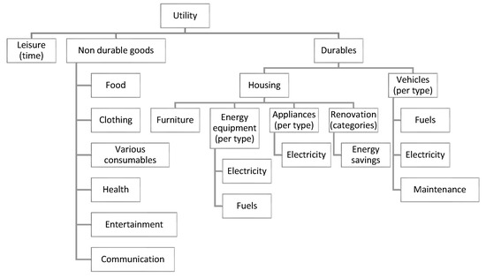
Figure 2.
Schematic representation of the GEM-E3-R nesting scheme for private consumption.
The general form of the LES formulation for a household in country involves minimum subsistence amounts and marginal utility parameters for every consumption by product category () and savings. Savings can be considered as utility-enabling with zero subsistence amounts. The constraint represents income, which partly depends on labour supply. The utility function has the following general form (often called Stone-Geary utility function):
Consumption is valued at market prices, assuming that households are price-takers, and savings are valued using a subjective discount rate influenced by market interest rates.
2.2.3. The Regional Economic Equilibrium Model
The purpose of the sub-country layer (SCL) model is to downscale the projections of the country-wide (CL) model to the regions. The SCL model includes the following main formulations for downscaling: (i) the SCL model determines the regional location of population/labour and production capacities of sectors depending on the relative attractiveness of the regions; (ii) given the regional endowment of primary production factors, the SCL model calculates production, consumption, income, and bilateral trade at a regional level; (iii) given regional production, the SCL model determines the accumulation of factors (state variables) that affect the valuation of amenities and dis-amenities of regions, which further influence the attractiveness of the regions in a subsequent time period; (iv) given sectoral activity and labour of regions, the model calculates inter-regional flows of goods and services and commuting.
Households derive utility from the consumption of goods and services, as well as from local amenities. The indirect utility (i.e., the maximum utility under income constraint) depends on prices of goods (), wages , price of capital (), and the amenities and dis-amenities measured by a vector , which is an aggregation of the individual amenities and dis-amenities forming an attractiveness index, as follows (where is a functional form formulated as a LES utility function). Increasing amenities implies higher utility, while the opposite holds for dis-amenities.
Cost of production by sector of activity depends not only on the prices of primary factors of production and the prices of other intermediate inputs, but also on local amenities and dis-amenities, which influence the productivity of factors. Also, the amenities influence the attractiveness of a region for the location of a new productive investment. Thus, the amenities influence the location of production activities dynamically. Similar mechanisms can be found in References [33,40,41,43]. The indirect cost function (i.e., the minimum cost for given volume of output) depends on factor prices, such as wages (), cost of capital (), and the prices of intermediate goods and services (), as well as on amenities, denoted by a vector , that is an aggregation of the individual amenities and dis-amenities forming an attractiveness index.
The aggregation of amenities () forming the attractiveness index employs a CES (constant elasticity of substitution) non-linear function , having slopes that are increasing for amenities and decreasing for dis-amenities. The function is linearized in the calibration of the model, as a linear combination of amenity values weighted by marginal utilities attributed to the amenities.
Similarly, the amenities () that influence production costs form the attractiveness index for industries using a constant elasticity of substitution (CES) aggregation function , having slopes that are increasing for amenities and decreasing for dis-amenities. The function is linearized in the model calibration as a linear combination of amenity values weighted by the marginal productivities attributed to the amenities.
In the above formulas, the use of CES aggregation functions implies a non-perfect substitution among amenities.
The model valuates the regional amenities using stock-flow equations that involve state-variables and accumulation of resources (). The changes in stock variables, , affect the value of amenities non-linearly to capture economies or dis-economies of scale that further influence location choices. The stock variables depend on these location choices dynamically over time. The relationship between stock variables and amenity values follows a Fréchet function to capture saturation and acceleration effects, depending on parameter values, as in Reference [36].
Among, the stock and resource variables, it is worth mentioning that transport possibilities among regions is among the drivers of location choices, depending on transport infrastructure, congestion, and transport costs, as in References [55,56]. The model quantifies a regional accessibility index, formulated as a Cobb-Douglas aggregation function, to measure accessibility of a region , depending on explanatory factors denoted by the vector .
The location choices are discrete when decided by individual households and firms. At the aggregate level, the model calculates the frequencies of discrete choices by households and thus captures heterogeneity of preferences and technologies, including for the location decisions of households and firms. The model formulates the frequency of location choices and not the discrete choices to represent idiosyncratic preferences, as in References [36,37]. The frequencies of location choices follow a Gumbel probability distribution function, which depends on the valuation of utility-enabling attributes, such as amenities and dis-amenities that form regional attractiveness. The combination of idiosyncratic preferences and returns to scale linking amenities to state variables can lead to regional specialization and non-convergence of the regions, as in References [57,58,59]. The combination of the discrete choice model for locations and the dynamic stock-flow relationships constitutes the agglomeration and dispersion mechanisms formulated in the regional economic model.
The abovementioned formulation of amenities and their valuation influenced by the dynamics of state variables concerns the choice of regional location of investment and labour, but not the choice of investment in infrastructure. The latter has social and environmental effects that also affect the state variables. However, the model captures only the positive effects of investment in infrastructure, which derive from improved accessibility of a region. Other works in the literature, such as Reference [60], evaluate social, environmental, and other factors in the choice of investment infrastructure.
The model employs a generalized extreme value (GEV) distribution function to derive the frequencies of location choices. In other words, the indirect utility and the cost functions follow a GEV distribution, as in Reference [37]. Thus, the frequency of choosing region as a location by households and firms is as follows, where represent scale parameters and are elasticities:
The model uses a dynamic partial adjustment mechanism, which applies the desired location, seen in Equation (10), gradually over time. In this manner, the model avoids abrupt changes of location.
Among the attributes influencing the choice of location, we mention the following:
- The human capital availability which is approximated by skilled labour;
- Physical capital availability;
- Capital profitability which is approximated by the ratio of the investment cost to the rental price of capital;
- Natural resources (the model maps the resource-based activities to the location of the natural resources);
- Vertical integration which simulates the incentive of certain industries to form clusters;
- The market size, which is often mentioned as the home market effect in the New Trade theory.
The choice of location of households is also assumed to be influenced by the environmental quality, approximated by the CO2 emissions per NUTS-3 zone, disposable income, and population density. We use the CO2 emissions, calculated by the model, as a proxy of air pollution in a region, as CO2 is due to the combustion of fossil fuels, which is the source of air pollutants, such as sulphur, nitrogen oxides, and particulates. The transport-related indicators, which influence the location choice of both businesses and individuals, are used to evaluate the accessibility index by region.
The formulation of regional attractiveness captures the following important aspects of regionalization: (i) positive externalities stemming from agglomeration due to the coexistence of certain activities (e.g., activity specialization and industrial integration, cities as enablers of social networks, regions able to attract highly skilled labour, etc.); (ii) negative externalities in relation to resources and cross-effects among state variables (e.g., conflicts between tourism and heavy industry); and (iii) limitations deriving from geography, transport or infrastructure (e.g., regions adjacent to more than one country having higher opportunities to attract activity compared to peripheral regions).
Once located, the households supply labour both to local and adjacent regional markets, depending on relative wages and the commuting time. The commuting part of the labour force among any pair of adjacent regions is determined according to:
Equation (11) also draws on discrete choice theory. The attributes influencing the choices include the regional wages and the commuting costs that further depend on transportation and time costs . The formula uses as weights reflecting the habits of commuters and the elasticity representing the easiness of commuting and the influence of other factors. The model adds transport costs and cost of time for commuting to workplaces as factors that influence residence location in relation to the workplace. The spatial resolution of this representation is, however, too aggregated to represent commuting adequately. However, data limitations and computational complexity do not allow going deeper than the NUTS-3 regional segmentation.
The model considers that the regional origin defines distinct varieties of goods and services, and thus applies imperfect substitution among goods of different regional origin. Both the households and the production sectors determine demand for the regional varieties as part of the nested choices. The choice of varieties depends on relative costs that reflect regional economic features and transport costs, depending also on accessibility. When transport infrastructure develops and improves the accessibility of a region, transport costs reduce, which implies that the menu of varieties available for selection is enlarged, inducing efficiency gains in the aggregation of varieties. The mechanism is similar to the love-of-variety formulation used in economic trade models, which were firstly specified by Dixit and Stiglitz, see Reference [61], as illustrated by the equation below.
The frequency of an investment by sector to be implemented in a region follows a GEV distribution function depending on the attractiveness index , as seen by the sector that aggregates the values of the various features of the region (costs, proximity to resources, access to cheap labour or adequate skills and transport costs) entering the cost function .
The locational choices for investment determine the capital stock dynamically, which acts as a constraint on regional production in the next period. The funding of investment expenditures by region has to match investment expenditures within the same sector, as calculated at a country level. Public investment and consumption are exogenously allocated to regions. Likewise, to the national part of the model, investment by sector implies demand for equipment goods and construction, based on fixed technical coefficients.
To calculate interregional trade flows, the regional economic model employs a formulation based on distances and transportation costs, as well as on production costs and behavioural parameters, the latter representing preferences. The formulation aims to capture the influence of several factors, such as infrastructure development, transport technologies and fuel costs, and the possible improvement in the accessibility of regions. The calculation of trade flows is performed step-wise:
- At the first stage, imports are differentiated by country of origin (i.e., intra-national imports versus international imports);
- At the second stage, the consumption of imported goods is further disaggregated into consumption by region of origin.
The equation below illustrates the calculation of trade flows, , of product between regions and .
The equation relates the share of trade flow from to over product demand in the market to the regional share of product in production in the country of origin and the cost factors that include transport costs, and relative regional prices. The elasticity represents trade impediments and imperfect substitution of product varieties depending on the origin. The transport costs derive as the weighted average cost of transport modes including cost of time.
The regional economic equilibrium model is a very large mathematical problem, as it covers NUTS-3 (approximately 3000 regions) and 37 goods and services per country. For a non-linear mixed complementarity problem of this size, computational limitations are considerable (mainly memory limits). To overcome the computational difficulties, we apply an iterative algorithm consisting of running the regional model per region in a parallel computing framework, assuming interregional flows as given in intermediate steps and applying a collection of the results for the regions to run the gravity model for all regions simultaneously and, thus, derive the interregional flows. The adjusted flows update the fixed interregional exchanges in the isolated regional models which run again in parallel. The iterations continue over time using the stock-flow relations, which concern capital stock, labour, and the state and stock variables that affect the valuation of amenities, hence, the attractiveness of regions that are adjusting dynamically.
3. Model Application
This section presents an application of the regional economic equilibrium model to an impact assessment of development of electrification of cars and the recharging infrastructure. The transport restructuring case also involves the development of advanced technology biofuels and reduction in the use of oil products. The parameters for transport sector restructuring came from simulations using the PRIMES–TREMOVE model.
Firstly, we quantify a base case scenario that excluded electrification and biofuels. Then, we quantify the transport sector restructuring case regarding economic and regional impacts. We draw conclusions from the comparison of the restructuring scenario to the base case.
The model’s regional dataset has limitations: not all data on NUTS-3 regional resolution are real (statistically observed) for all activity locations. Part of the dataset on NUTS-3 results from calibration techniques, mainly using a gravity model. The model results presented in this chapter are subject to further fine tuning to improve the realism for specific regions.
3.1. Base Case Scenario
The base case scenario uses various exogenous sources regarding the evolution of the population, labour force, and productivity. The data sources were the European Commission’s 2018 Ageing report, see Reference [62], United Nations demographic projections, International Labour Organisation projections of labour force, and various forecasts by the International Monetary Fund, World Bank, and others. At the sub-country level, population projection also used data from Eurostat.
3.2. Policy Scenario for the Transport Sector
The electrification of mobility (mainly cars, light-duty vehicles, buses, and rail) and the use of sustainable biofuels (advanced technology based on lignocellulosic feedstock) are the results of transport sector simulations using PRIMES–TREMOVE for scenarios that meet the EU targets for 2030, as in References [3,4]. During the early stages of the transition towards industrial maturity, electric vehicle technologies and batteries have rather short travelling ranges. Consumers hesitate purchasing electric cars unless they see that a battery recharging network has a sufficient geographic coverage. The transport restructuring scenario assumes development of recharging infrastructure in stages along with the expansion of the market for electric vehicles. Within the scenario logic, the electric car and battery manufacturing industries anticipates the market development and invests. Thus, the industry experiences a decrease in the costs of cars and batteries along the learning-by-doing curve. Cost reductions further enable higher consumers’ uptake dynamically. The quantification of learning-by-doing dynamics and the ensuing decrease in costs of batteries and biofuels are exogenous assumptions, using information coming from the transport sector restructuring scenarios based on the PRIMES–TREMOVE model. Several scenario variants are available to explore different cost evolutions. In most of the scenarios, high learning rates imply that the levelized cost of electric cars becomes lower than for internal combustion cars in the long term. However, the industry needs time to tap into the learning benefits and the horizon to 2030 is rather short for achieving the full learning potential. The main policy measures are the continuous decrease in the CO2 car standard and the development of recharging infrastructure.
The agricultural sectors benefits from the development of biofuels from lignocellulosic feedstock converted into fungible hydrocarbons using Fischer–Tropsch technology. This technology is sustainable and does not use food-related feedstock. The agricultural sectors will thus see increased activity to supply the biomass feedstock domestically. The electric goods sector produces batteries for electric vehicles and components used in the recharging system. The car manufacturing industry produces the vehicles. The recharging infrastructure requires goods from the metals industry, electronics, other equipment goods industries, and services. Finally, the sectors supplying public passenger transport services, especially rail, will also see increased demand due to modal shifts. The oil industry, including the sectors of oil refining and the distribution of liquid fuels, will see a reduction in demand and a declining activity, despite maintaining the use of oil in other sectors, notably in petrochemicals.
Fiscal revenues will be affected by the restructuring in transport, as revenues from excise taxes on oil products will decrease and cannot be replaced by tax revenues from excise taxes on biofuels and electricity. Currently the latter taxes are small and are unlikely to increase in the future to continue supporting market penetration of alternative fuels. The increased domestic activity induced by the production of biofuels, electric vehicles, and grid components will drive tax revenues upwards, but the tax rates will be relatively low compared to the taxation of oil products. Given that the model includes an endogenous mechanism to achieve equilibrium in public finances, other taxes will have to rise to compensate for the loss in revenue, in the case taxation is low, or subsidies will have to be applied on alternative fuels and technologies.
To illustrate the model’s properties, we present below a scenario to the horizon of 2030, which assumes that five Member States of the EU promote electric cars by means of carbon dioxide emissions standard, apply efficiency standards to reduce energy consumption in public and freight transport and impose blending mandates to increase the share of biofuels in liquid fuels. Also, other measures promote the use of rail among the competing modes of freight transport. The implied changes can be seen in Table 3, Table 4 and Table 5.
Table 3.
Market shares of vehicle technology types in 2030.
Table 4.
Shares of fuels and electricity in public passenger and freight transport in 2030.
Table 5.
Share of biofuels.
The countries under consideration were: Austria (AT), Germany (DE), Italy (IT), the Netherlands (NL), and the United Kingdom (UK). These regions were further decomposed at the sub-country level: Austria was decomposed into nine regions; the Netherlands into 12; United Kingdom into 42; Italy into 21; and Germany into 38. These regions cover approximately 46% of the EU28 population, account for 47% of the European GDP, and 39% of transport-related energy consumption, according to Eurostat regional statistics, see Reference [63].
The policy scenario projections show that the policies enable fuel switching in favour of biofuels and electricity, increase the share of electromobility cars and the use of rail, while reduce demand for oil products. The total reduction in oil consumption in the six countries is 12% in 2025 and 20% in 2030, compared to the base case.
3.3. Results of the Country-Wide Economic Equilibrium Model
Table 6 summarizes the macroeconomic impacts of the transport policy scenario on the national economies, showing percentage changes of macroeconomic variables relative to the base case projection.
Table 6.
Macroeconomic implications of the policy scenario at the country-wide level.
In general, the macroeconomic impacts are small in magnitude. The impacts on GDP and total investment are slightly negative in all countries except for the Netherlands, but they are slightly positive for private consumption and employment. Both exports and imports slightly increase except for the imports in the Netherlands.
The transport sector restructuring essentially replaces imported oil products by alternative fuels, such as electricity and biofuels, produced domestically and increases the manufacturing of equipment, also domestically. The direct effects are positive for domestic activity in the production sectors, hence, also for employment and investment. However, the scenario technology cost assumptions imply a small increase in the levelized cost (i.e., total cost per unit of transport activity including capital, fixed, and operation costs) of transport services, both for public and private transport, compared to the costs in the base case. The increase in costs derives from the assumption that biofuels are more expensive than oil products and electric cars are more expensive than conventional ones in terms of levelized costs, because the scenario assumes that the horizon until 2030 is rather short and will not allow for fully tapping onto the learning potential. In the logic of the same transport scenario, electric cars achieve levelized costs below those of conventional cars after 2030. The increase in costs is small up to 2030, but still significant enough to induce crowding out effects. The aim of our macroeconomic and regional impact assessment is however to demonstrate that activity and employment may possibly see positive developments at least in several regions despite the increase in transport costs during the early stages of the transition.
Crowding out effects are shifts in the use of revenues by households and firms, and losses of competitiveness in foreign trade. Increased cost of transport implies that households and firms have less money to spend on other products and services and for durable goods and investment. As the period until 2030 is rather short to allow full exploitation of the learning potential of the new technologies, the transition period is costly for transport services and so the induced productivity improvement does not allow the economy to regain full competitiveness and offset the crowding out effects.
The shift away from oil products favours sectors that are more labour intensive than the oil industry. Such sectors are agriculture, which produces biofuels, and equipment goods industries, which produce vehicles and electric components. Service sectors also benefit from the same substitution and are also labour intensive. Shifting activity towards sectors with high labour intensity is favourable for employment and private consumption due to the increased revenues from both the rise in employment and wage rates, as lower unemployment implies higher wage rates. At the same time, shifting away from capital-intensive sectors implies lower overall investment, as investment per unit of production is slightly lower in labour-intensive sectors compared to capital-intensive ones.
Consequently, the rise in domestic activities drives an increase in GDP. Labour intensity also increases GDP thanks to private consumption but crowding out effects due to the increase in transport costs imply losses of GDP. The net effect on GDP may be positive or negative depending on the particular conditions prevailing in each country. However, the negative effects seem to be slightly higher than the positive ones, because the period up to 2030 is rather short and does not allow the full attainment of the learning-by-doing potential for alternative vehicle and fuel technologies. Higher learning in the long term would allow for a reduction of the effects on transport costs, thus, an offset of the negative economic impacts due to the crowding out effects. The positive effects from the rise in activity would then overcompensate for the cost effects and, thus, impacts on GDP, investment, and employment turn positive in the longer term. Needless to say, if we assume that electric cars have a lower levelized cost than conventional ones already before 2030, the economic effects would become positive throughout. This equally applies to biofuels.
3.4. Results of the Regional Economic Equilibrium Model
The regional economic effects are found not uniform across the regions (Figure 3, Figure 4, Figure 5 and Figure 6). They depend on several features of the regional economies, which mainly concern the specializations and the resource endowments of the regions. A region with resources able to produce biofuels will see a rise in activities that would be beneficial to the regional economy, activity, income, and employment via the multiplier effect. A similar benefit can be seen in regions that have specialized industries producing vehicles and electric components or batteries. Wage rates may increase in regions benefiting from labour-intensive activities, such as production of biofuels and equipment goods and, thus, private consumption will increase but some sectors, notably services, may be negatively affected by the rise of wages. But probably, the rise on demand would offset the negative impacts on service sectors. The rise in wages and employment will make regions more attractive for labour location but migration will reduce the pressure on wages dynamically.
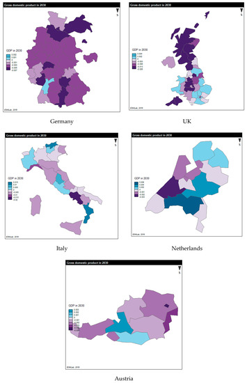
Figure 3.
Percentage change of regional GDP to the base case in 2030.
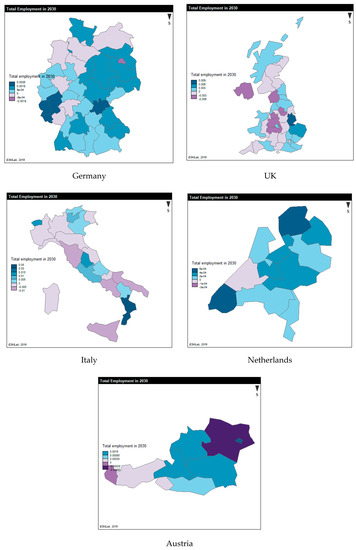
Figure 4.
Percentage change in regional employment to the base case in 2030.
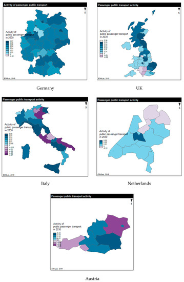
Figure 5.
Percentage change in public passenger transport relative to the base case in 2030.
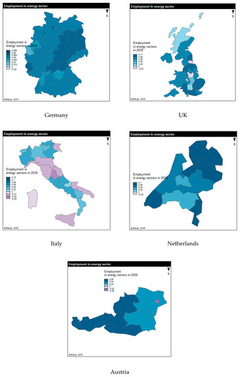
Figure 6.
Percentage change in employment in energy industries relative to the base case in 2030.
The regional model determines transport activity by mode also at the NUTS-3 level. The restructuring implies an increase in public passenger transport to the detriment of private transport. The increase in rail transport in most regions in Germany and the United Kingdom was found to be between 9% and 14% compared to the base case.
The decrease in the consumption of oil products implies a decrease in oil refining and distribution. Oil refining is located in few regions, which would see a significant reduction in activity. At the same time, consumption, hence production of electricity, increases and the regions are positively affected in this case. Other regions lose oil refining activities. Biofuels also substitute oil products and, thus, agriculture production rises. Facilities would emerge in many regions for converting biomass feedstock to bio-gasoline and bio-diesel.
The negative impact on employment in the oil industry would be offset by the increased activity in the electricity sector, in particular, because the increase in renewable sources for power generation involves higher employment than in the oil industry.
4. Conclusions
In this paper, we present a regional and national economic equilibrium model, which incorporates detailed representations of transport and energy and their inter-linkages with the economy. The model is numerically applied to the entire EU with a split in NUTS-3 regions. The country-wide model layer represents the EU countries integrated into the global economy and distinguishes between many sectors of activity and countries.
The regional model (second layer) uses economic growth, primary factor endowment, and budget resources as constraints resulting from the national level model and allocates labour, investment, consumption, and sectoral activity to the regions based on their relative attractiveness, which are endogenously derived from model variables. Inter-regional flows are also derived endogenously from the location of primary resources and the relative competitiveness of industries. The regional location of primary factors, such as labour and capital, the attractiveness of the regions, and the competitiveness driving inter-regional flows depend on transportation costs and conditions, including time and convenience. The entire two-layer (national and regional) model is fully dynamic with stock-flow equations adjusting labour, capital, resources, and the state-variables influencing regional attractiveness.
The regional economic impact assessment is the purpose of the new model. The study of transport restructuring is derived from more detailed transport models, such as PRIMES–TREMOVE which are used to prepare the inputs of the regional economic model.
The transport sector affects the regional economy when transport sector restructuring requires investment in infrastructure, activity to produce biofuels and electricity that substitute for oil products, as well as manufacturing of new technologies such as electric vehicles, batteries and recharging networks. The numerical applications of the two-layer model demonstrate that transport sector restructuring has significant impacts on regional activity and employment that are not uniform across the regions. The two-layer approach in regional economic modelling proved to be robust and important for improving the realism of regional agglomeration.
The paper illustrates a model application in the assessment of economic impacts of electrification of mobility in Europe in conjunction with policies promoting biofuels and facilitating modal shifts in favour of rail both for passengers and freight. The EU decarbonization strategy for the transport sector has such priorities. The alternatives replacing fossil oil in transport are more labour-intensive, boost activity also in regions, but lead to slight increase in transport costs, which exert crowding out effects on the economy, albeit of small magnitude. The net impact on regions’ GDP can be negative or positive depending on regional specialization and resource endowment. Regions with fossil fuel activities see negative impacts and regions developing manufacturing of new equipment, production of electricity or agriculture producing biofuels benefit from the restructuring.
The development and computer implementation of the model has been tedious regarding data collection and computational burden. The regional datasets were not complete in Europe and so we plan to further improve our calibration techniques, mainly gravity models, regarding localization of activities in regions in a base-year. The size of the model is prohibitively large even for high-end computers. We had then to decompose the model and apply iterative techniques to achieve reasonable computer times. The computational difficulties have not allowed us to run the model intertemporally but only in a time forward manner with adjusting dynamics. Improving the foresight features of the model is in our model development agenda.
Further development of the regional economy–energy and transport model are in our ongoing research. The agenda includes data improvement, fine tuning of the features of the various non-linear choice functions, extension of the modelling of amenities, and the implementation of a more efficient computer system and solution algorithm.
Author Contributions
Conceptualization, P.C. and P.K.; software and data curation, I.C. and P.K.
Funding
The authors acknowledge partial funding by the European Commission, project TRIMODE, Contract No 30-CE-0746521/00-34.
Conflicts of Interest
The authors declare no conflicts of interest.
References
- European Environmental Agency. Greenhouse gas emissions from transport. Available online: https://www.eea.europa.eu/data-and-maps/indicators/transport-emissions-of-greenhouse-gases/transport-emissions-of-greenhouse-gases-11 (accessed on 15 May 2019).
- European Commission, EU Science Hub. Available online: https://ec.europa.eu/jrc/en/research-topic/transport-sector-economic-analysis (accessed on 15 May 2019).
- White Paper 2011—Roadmap to a Single European Transport Area; European Commission: Brussels, Belgium, 2011; Available online: https://ec.europa.eu/transport/themes/strategies/2011_white_paper_en (accessed on 15 June 2019).
- European Commission. Clean Planet for All a European Long-Term Strategic Vision for a Prosperous, Modern, Competitive and Climate Neutral Economy, In-Depth Analysis in Support of the Commission Communication; COM/2018/773 A; European Commission: Brussels, Belgium, 2018. [Google Scholar]
- Capros, P.; Siskos, P. PRIMES-TREMOVE Transport Model. Available online: https://ec.europa.eu/clima/sites/clima/files/strategies/analysis/models/docs/primes_tremove_en.pdf (accessed on 15 May 2019).
- Bröcker, J.; Mercenier, J. General equilibrium models for transportation economics. In A Handbook of Transport Economics; Palma, D.A., Lindsey, R., Quinet, E., Vickerman, R., Eds.; Edward Elgar Publishing: Cheltenham, UK, 2011; pp. 21–45. [Google Scholar] [CrossRef]
- Robson, E.N.; Wijayaratna, K.P.; Dixit, V.V. A review of computable general equilibrium models for transport and their applications in appraisal. Transp. Res. Part A Policy Pract. 2018, 116, 31–53. [Google Scholar] [CrossRef]
- Rietveld, P. Spatial economic impacts of transport infrastructure supply. Transp. Res. Part A Policy Pract. 1994, 28, 329–341. [Google Scholar] [CrossRef]
- Oosterhaven, J.; Knaap, T. Spatial Economic Impacts of Transport Infrastructure Investments. In Transport Projects, Programmes and Policies; Nellthorp, J., Mackie, P., Pearman, A., Eds.; Routledge: Abingdon, UK, 2003. [Google Scholar] [CrossRef]
- Donaldson, D. Railroads of the Raj: Estimating the Impact of Transportation Infrastructure. Am. Econ. Rev. 2018, 108, 899–934. [Google Scholar] [CrossRef]
- Redding, S.J.; Matthew, A.T. Transportation costs and the spatial organization of economic activity. In Handbook of Regional and Urban Economics; Duranton, G., Henderson, J.V., Strange, W.C., Eds.; Elsevier: Amsterdam, The Netherlands, 2015; Volume 5, pp. 1339–1398. [Google Scholar] [CrossRef]
- Partridge, M.D.; Rickman, D.S. Regional Computable General Equilibrium Modeling: A Survey and Critical Appraisal. Int. Reg. Sci. Rev. 1998, 21, 205–248. [Google Scholar] [CrossRef]
- Bradley, J.; Gács, J.; Kangur, A.; Lubenets, N. HERMIN: A macro model framework for the study of cohesion and transition. In Integration, Growth and Cohesion in an Enlarged European Union; Bradley, J., Petrakos, G., Traistaru, I., Eds.; Springer: New York, NY, USA, 2007; pp. 207–242. [Google Scholar]
- Ivanova, O.; Heyndrickx, C.; Spitaels, K.; Tavasszy, L.; Manshanden, W.; Snelder, M.; Koops, O. RAEM: Version 3.0; Final Report; Transport & Mobility: Leuven, Belgium, 2007; p. 77. [Google Scholar]
- Donaghy, K. CGE Modelling in space. In Handbook of Regional Growth and Development Theories; Capello, R., Nijkamp, P., Eds.; Edward Elgar: Cheltenham, London, UK, 2009; pp. 389–422. [Google Scholar]
- Ivanova, O.; Kancs, D. Rhomolo: A Dynamic General Equilibrium Modelling Approach to the Evaluation of the EU’s Regional Policies. In EERI Research Paper Series 2010/28; Economics and Econometrics Research Institute (EERI): Brussels, Belgium, 2010. [Google Scholar]
- Varga, A.; Jarosi, P.; Sebestuen, T. Modelling the economic impacts of regional R&D subsidies: The GMR-Europe model and its application for EU Framework Program policy impact simulations. In Proceedings of the 6th Regional Innovation Policy Seminar, Circle, Lund, Sweden, 13–14 October 2011. [Google Scholar]
- Di Comite, F.; Kancs, D. Modelling of Agglomeration and Dispersion in RHOMOLO; No. JRC81349; Joint Research Centre (Seville Site): Sevilla, Spain, 2014. [Google Scholar]
- Brandsma, A.; Kancs, D.; Monfort, P.; Rillaers, A. RHOMOLO: A dynamic spatial general equilibrium model for assessing the impact of cohesion policy. Pap. Reg. Sci. 2015, 94, 197–221. [Google Scholar] [CrossRef]
- Giesecke, J.A.; Madden, J.R. Regional Computable General Equilibrium Modeling. In Handbook of Computable General Equilibrium Modeling; Dixon, P.B., Jorgenson, D.W., Eds.; Elsevier: Amsterdam, The Netherlands, 2013; pp. 379–475. [Google Scholar] [CrossRef]
- Partridge, M.D.; Rickman, D.S. Computable General Equilibrium (CGE) Modelling for Regional Economic Development Analysis. Reg. Stud. 2010, 44, 1311–1328. [Google Scholar] [CrossRef]
- Tavasszy, L.A.; Thissen, M.J.P.M.; Oosterhaven, J. Challenges in the application of spatial computable general equilibrium models for transport appraisal. Res. Transp. Econ. 2011, 31, 12–18. [Google Scholar] [CrossRef]
- Leontief, W.; Morgan, A.; Polenske, K.; Simpson, D.; Tower, E. The Economic Impact--Industrial and Regional—Of an Arms Cut. Rev. Econ. Stat. 1965, 47, 217–241. [Google Scholar] [CrossRef]
- Dixon, P.B.; Parmenter, B.R.; Sutton, J. Spatial Disaggregation of Orani Results: A Preliminary Analysis of the Impact of Protection at the State Level. Econ. Anal. Policy 1978, 8, 35–86. [Google Scholar] [CrossRef]
- Dixon, P.B.; Rimmer, M.T.; Tsigas, M.E. Regionalising results from a detailed CGE model: Macro, industry and state effects in the U.S. of removing major tariffs and quotas. Pap. Reg. Sci. 2007, 86, 31–55. [Google Scholar] [CrossRef]
- Horridge, M.; Madden, J.; Wittwer, G. The impact of the 2002–2003 drought on Australia. J. Policy Modeling 2005, 27, 285–308. [Google Scholar] [CrossRef]
- Muth, R. Migration: Chicken or Egg? South. Econ. J. 1971, 37, 295–306. [Google Scholar] [CrossRef]
- Polinsky, M.A.; Shavell, S. Amenities and property values in a model of an urban area. J. Public Econ. 1976, 5, 119–129. [Google Scholar] [CrossRef]
- Rosen, S. Wage-based indexes of urban quality of life. In Current Issues in Urban Economics; Mieszkowski, P., Straszheim, M., Eds.; Johns Hopkins University Press: Baltimore, MD, USA, 1979; pp. 74–104. [Google Scholar]
- Greenwood, M.J. Research on Internal Migration in the United States: A Survey. J. Econ. Lit. 1975, 13, 397–433. [Google Scholar]
- Greenwood, M.J.; Hunt, G.L. Econometrically accounting for identities and restrictions in models of interregional migration. Reg. Sci. Urban Econ. 1984, 14, 113–128. [Google Scholar] [CrossRef]
- Graves, P.E.; Mueser, P.R. The role of equilibrium and disequilibrium in modelling regional growth and decline: A critical reassessment. J. Reg. Sci. 1993, 33, 69–84. [Google Scholar] [CrossRef] [PubMed]
- Partridge, M.D.; Rickman, D.S.; Ali, K.; Olfert, M.R. The geographic diversity of U.S. nonmetropolitan growth dynamics: A geographically weighted regression approach. Land Econ. 2008, 84, 241–266. [Google Scholar] [CrossRef]
- Roback, J. Wages, rents, and the quality of life. J. Political Econ. 1982, 90, 1257–1278. [Google Scholar] [CrossRef]
- Roback, J. Wages, rents, and amenities—Differences among workers and regions. Econ. Inq. 1988, 26, 23–41. [Google Scholar] [CrossRef]
- Redding, J.S.; Rossi-Hansberg, E. Quantitative Spatial Economics. Annu. Rev. Econ. 2016, 9, 21–58. [Google Scholar] [CrossRef]
- Monte, F.; Redding, J.S.; Rossi-Hansberg, E. Commuting, migration, and local employment elasticities. Am. Econ. Rev. 2018, 108, 3855–3890. [Google Scholar] [CrossRef]
- Brueckner, J.K.; Thisse, J.-F.; Zenou, Y. Why is central Paris rich and downtown Detroit poor? An amenity-based theory. Eur. Econ. Rev. 1999, 43, 91–107. [Google Scholar] [CrossRef]
- Judson, D.H.; Reynolds-Scanlon, S.; Popoff, C.L. Migrants to Oregon in the 1990’s: Working age, near-retirees, and retirees make different destination choices. Rural Dev. Perspect. 1999, 14, 24–31. [Google Scholar]
- Beyers, W.B.; Lindahl, D.P. Lone eagles and high fliers in rural producer services. Rural Dev. Perspect. 1996, 11, 2–10. [Google Scholar]
- Johnson, J.D.; Rasker, R. Local government: Local business climate and quality of life. Mont. Policy Rev. 1993, 3, 11–19. [Google Scholar]
- Clark, D.E.; Hunter, W.J. The impact of economic opportunity, amenities and fiscal factors on age-specific migration rates. J. Reg. Sci. 1992, 32, 349–365. [Google Scholar] [CrossRef]
- Poudyal, N.C.; Hodges, D.G.; Cordell, H.K. The role of natural resource amenities in attracting retirees: Implications for economic growth policy. Ecol. Econ. 2008, 68, 240–248. [Google Scholar] [CrossRef]
- McGregor, P.G.; Swales, J.K.; Yin, Y.P. A long-run interpretation of regional input-output analysis. J. Reg. Sci. 1996, 36, 479–501. [Google Scholar] [CrossRef]
- Kim, E.; Kim, K. Impacts of the development of large cities on economic growth and income distribution in Korea: A multiregional CGE model. Pap. Reg. Sci. 2003, 82, 101–122. [Google Scholar] [CrossRef]
- Bröcker, J.; Korzhenevych, A. Forward looking dynamics in spatial CGE modelling. Econ. Model. 2013, 31, 389–400. [Google Scholar] [CrossRef]
- Capros, P.; Van Regemorter, D.; Paroussos, L.; Karkatsoulis, P.; Fragkiadakis, C.; Tsani, S.; Charalampidis, I.; Revesz, T. GEM-E3 Model Documentation; JRC Working Papers JRC83177 2013; Joint Research Centre (Seville Site): Sevilla, Spain, 2013. [Google Scholar] [CrossRef]
- Karkatsoulis, P.; Siskos, P.; Paroussos, L.; Capros, P. Simulating deep CO2 emission reduction in transport in a general equilibrium framework: The GEM-E3T model. Transp. Res. Part D Transp. Environ. 2017, 55, 343–358. [Google Scholar] [CrossRef]
- Fragkos, P.; Tasios, N.; Paroussos, L.; Capros, P.; Tsani, S. Energy system impacts and policy implications of the European Intended Nationally Determined Contribution and low-carbon pathway to 2050. Energy Policy 2017, 100, 216–226. [Google Scholar] [CrossRef]
- Capros, P.; Paroussos, L.; Charalampidis, I.; Fragkiadakis, K.; Karkatsoulis, P.; Tsani, S. Assessment of the macroeconomic and sectoral effects of higher electricity and gas prices in the EU: A general equilibrium modeling approach. Energy Strategy Rev. 2016, 9, 18–27. [Google Scholar] [CrossRef]
- Karkatsoulis, P.; Capros, P.; Fragkos, P.; Paroussos, L.; Tsani, S. First-mover advantages of the European Union’s climate change mitigation strategy. Int. J. Energy Res. 2016, 40, 814–830. [Google Scholar] [CrossRef]
- Shahrokhi Shahraki, H.; Bachmann, C. Designing computable general equilibrium models for transportation applications. Transp. Rev. 2018, 1–28. [Google Scholar] [CrossRef]
- Blanchflower, D.G.; Oswald, A.J. The Wage Curve; The MIT Press: Cambridge, MA, USA, 1994. [Google Scholar]
- Armington, P. A Theory of Demand for Products Distinguished by Place of Production. Staff Pap. Int. Monet. Fund 1969, 16, 159–178. [Google Scholar] [CrossRef]
- Booth, D.E. Spatial patterns in the economic development of the Mountain West. Growth Chang. 1999, 30, 384–405. [Google Scholar] [CrossRef]
- Geurs, K.T. Transport Planning with Accessibility Indices in The Netherlands; Discussion Paper; International Transport Forum: Paris, France, 2018. [Google Scholar]
- Davis, D.R.; Dingel, J.I. The Comparative Advantage of Cities; Working Paper Series; National Bureau of Economic Research: Cambridge, MA, USA, 2014. [Google Scholar] [CrossRef]
- Gaubert, C. Firm Sorting and Agglomeration. National Bureau of Economic Research 2018; Working Paper Series; NBER, 1050 Massachusetts Ave.: Cambridge, MA, USA, 2018. [Google Scholar] [CrossRef]
- Redding, J.S. Estimating Neighborhood Effects: Evidence from War-Time Destruction in London. Available online: https://www.semanticscholar.org/paper/Estimating-Neighborhood-Effects-%3A-Evidence-from-in-Redding/30ac196f987a47e087697bc2e2daba43ab73a95b (accessed on 12 July 2019).
- Nesticò, A.; Sica, F. The sustainability of urban renewal projects: A model for economic multi-criteria analysis. J. Prop. Invest. Financ. 2017, 35, 397–409. [Google Scholar] [CrossRef]
- Dixit, A.K.; Stiglitz, J.E. Monopolistic Competition and Optimum Product Diversity. Am. Economic Review 1977, 67, 297–308. [Google Scholar]
- The 2018 Ageing Report: Underlying Assumptions and Projection Methodologies; European Commission: Brussels, Belgium, 2017.
- European Commission. Eurostat. Regional Statistics Database. Available online: https://ec.europa.eu/eurostat/web/regions/data/database (accessed on 15 May 2019).


© 2019 by the authors. Licensee MDPI, Basel, Switzerland. This article is an open access article distributed under the terms and conditions of the Creative Commons Attribution (CC BY) license (http://creativecommons.org/licenses/by/4.0/).