Improved Deadbeat FC-MPC Based on the Discrete Space Vector Modulation Method with Efficient Computation for a Grid-Connected Three-Level Inverter System

Abstract

The utilization of three-level T-type (3L T-type) inverters in finite set-model predictive control (FS-MPC) of grid-connected systems yielded good performance in terms of current ripples and total harmonic distortions. To further improve the system’s performance, discrete space vector modulation (DSVM) was utilized to synthesize a higher number of virtual voltage vectors. A deadbeat control (DBC) method was used to alleviate the computational burden and provide the optimum voltage vector selection. However, 3L inverters are known to suffer from voltage deviation, owing to the imbalance of the neutral-point voltage. We have proposed a simplified control strategy for balancing the neutral point in the FS-MPC with DSVM and DBC of grid-connected systems, not requiring a weighting factor or additional cost function calculation. The effectiveness of the proposed method was validated using simulation and experiment results. Our experimental results show that the execution time of the proposed algorithm was significantly reduced, while its current quality performance was not affected.

1. Introduction

Model predictive control (MPC) has become an attractive alternative for controlling power electronic applications, such as motor drives and power converters [1]. There are two main categories of MPC: (1) continuous MPC (CMPC), in which output is generated and delivered to a modulator, and (2) finite-set MPC (FS-MPC), which can control a finite number of feasible switching states using a predefined cost function [2,3,4,5]. Among the two types, FS-MPC is preferable, owing to its many advantages, such as the fast dynamic response, intuitive appeal, inclusion of constraints and nonlinearities, and easy implementation. However, an important drawback of the original method is its variable switching frequency and large current ripples, which requires the use of large passive filter components [2,6].

Numerous studies aiming to improve the performance of classical FS-MPC for both power converters and motor drives have been performed. To reduce current ripples and alleviate harmonic distortion, an attempt was made in [7,8] to increase the prediction horizon of FS-MPC. Although good performance was achieved, intensive experimentation is still necessary for determination of correct weighting factors and control horizons [8], which is computationally demanding [9]. A deadbeat solution was suggested in Reference [10] for a two-level voltage-source inverter, which allows the computational load of FS-MPC to be reduced by reducing the complete enumeration for the whole voltage vectors. Although this solution helped to address the problem of computational intensity, the large torque ripples could not be eliminated.

FS-MPC based on discrete space vector modulation (DSVM) was proposed in References [11,12] to reduce current ripples and guarantee a constant switching frequency. The main advantage of DSVM is that it allows the number of degrees of freedom to be increased by synthesizing various virtual voltage vectors in the space vector diagram [12]. Similarly to classical FS-PTC, the optimal voltage vector is selected to minimize the objective error in the respective cost function, and is applied to the inverter using space vector modulation (SVM). Nevertheless, the main issue associated with the DSVM approach is its high computational burden, owing to a large lookup table that holds the initialized virtual voltage vectors. To solve this problem, deadbeat control was utilized to consider a limited number of virtual voltage vectors, regardless of their number [13]. In this way, the calculation time was significantly reduced, making the method suitable for realistic applications.

Although two-level inverters (2L inverters) are extensively used for power converters and motor drives for generation of voltage vectors applied to terminals [14], they suffer from some issues. Two-level inverters require a very high switching frequency; hence, a higher harmonic current distortion is generated, owing to the limitation of voltage levels. In addition, the maximal DC link voltage is constrained due to the rating of the semiconductors. Therefore, multilevel inverters (ML inverters) have been considered an attractive solution capable of solving the above-mentioned problems and synthesizing output voltages with several discrete levels. Three-level inverters (3L inverters), such as neutral-point clamped (NPC) and T-type inverters, are the most prominent topologies of ML inverters. Compared with 2L inverters, the number of degrees of freedom for obtaining the voltage vectors is higher, which yields better current quality and better control. Despite the advantages of 3L inverters, neutral-point voltage balancing seriously affects their control performance [15], causing higher ripples and distortion of stator currents. Hence, 3L inverters require high-rated capacitors, owing to their unequal voltage distribution, which, in turn, results in a higher voltage stress on the semiconductor switches.

It is worth mentioning it is complicated to include a NPC voltage balance variable in the cost function when implementing DBC. Thus, an algorithm for the DC link capacitor voltage balance should be separately applied for proper 3L inverter operation [16,17,18,19,20]. For example, in Reference [16], a calculated zero-voltage sequence was used for neutral-point balancing, while in Reference [18], the time-offset injection method was used for the same purpose. In Reference [20], a deadbeat model of predictive control combined with the discrete space vector modulation method was used for grid-connected systems using T-type 3L inverters. Two cost functions were used: one for selecting the optimal voltage, and another for the compensated voltage offset, because the neutral-point voltage problem of 3L inverters cannot be included as a variable in the cost function, due to the use of DBC method. The optimal voltage vectors were then synthesized using the SVM method for the entire sampling duration. Nevertheless, the use of two cost functions increased the computational burden of the control system.

This paper proposes a simplified control method for balancing the neutral point in the FS-MPC with the DSVM and DBC of grid-connected systems. Therefore, unlike the approach in Reference [20], the proposed method does not require additional cost functions for balancing the capacitance voltage. The proposed method led to a significant reduction in computation time while maintaining the current quality performance. This method was simulated and experimentally verified on a grid-connected, three-level T-type voltage source inverter.

2. System Modeling

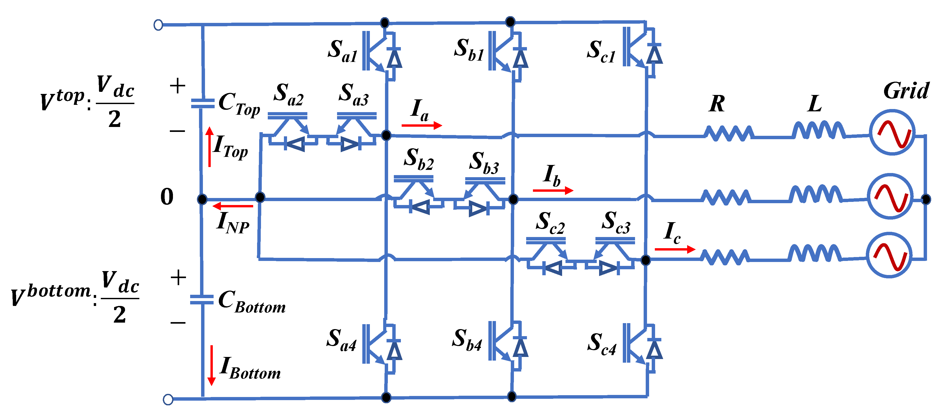
Essentially, there are three switching states for three-level topologies such as neutral-point clamped (NPC) and T-type inverters. Figure 1 shows the topology of a grid-connected, three-level T-type voltage source inverter. The output poles of the T-type inverter can be connected to three different levels of the source voltage, namely the positive bus bar “P,” the negative bus bar “N,” and the neutral point “0” [21]. With three-phase to two-phase transformation, the model of the inverter in the stationary d–q frame is given by:

$$u=R·\overrightarrow{i}+L·\frac{di}{dt}+e.$$

(1)

In Equation (1), R, L, u, i, and e, are the load resistance, filter inductance, inverter voltage vector, output current vector, and grid voltage vector, respectively. Because the top capacitance voltage (V^top) and the bottom capacitance voltage (V^bottom) can become unequal in the three-level voltage source inverter (VSI) (and hence will produce poor-quality output current and distorted output voltage), the capacitor voltages should be observed and taken into account at every time step, to ensure that they become balanced. The dynamic equations of the two capacitor voltages are given by:

$$V^{top}=V^{top}+I_{ NP}·\left(T_s/C\right)$$

(2)

$$V^{bottom}=V^{bottom}+I_{NP}·\left(T_s/C\right)$$

(3)

where C is the capacitance of each capacitor, $T_s$ is the sampling time, and I_NP is the neutral-point current.

3. FS-MPC Based DSVM with Deadbeat Control

3.1. Classical FS-MPC

The classical three-level FS-MPC uses only 19 voltage vectors as shown in Figure 2, defined by switching states, for prediction, and uses three stages: (1) estimation, (2) prediction, and (3) cost function optimization. An optimal control action is selected by minimizing a predefined cost function. All of the controlled objectives are included in the cost function in terms of errors; the errors are calculated by their respective references. The performance and the required computational burden of the model have been analyzed for the 3L T-type VSI.

To predict the future behavior of the inverter, the continuous-time model of Equation (1) should be approximated by a discrete-time model, using the normal forward Euler approximation with the sampling period T_s, as:

$$dy/dt=\left(y\left(k+1\right)-y\left(k\right)\right)/T_s.$$

(4)

Thus, the discretized models of current are given as:

$$i_{dq}\left(k+1\right)=i_{dq}\left(k\right)+\left(T_s/L\right)\left(u_{dq}\left(k\right)-R·i_{dq}\left(k\right)-e_{dq}\left(k\right)\right).$$

(5)

To predict i(k + 1) in Equation (5), i(k), e(k), and v(k) are required. The current i(k) is measured using the hardware sensors on the stationary d–q axis. Assuming that e(k) does not change much during T_s, e(k) can be estimated by shifting Equation (5) one step backward, as

$$e_{dq}\left(k\right)\approx e_{dq}\left(k-1\right)$$

(6)

$$e_{dq}\left(k\right)=u_{dq}\left(k-1\right)-\left(L/T_s\right)\left[\left(1-\left(R·T_s/L\right)\right)·i_{dq}\left(k\right)-i_{dq}\left(k-1\right)\right].$$

(7)

As it is evident that there is a one-step delay in the digital control system, the voltage vector at time k will not be applied until time k + 1. Therefore, to obtain the optimal voltage vector among the 19 voltage vectors, the cost function (CF) used to measure the errors between the references and the predictions in the stationary d–q frame was defined, as in Equation (8). To remove the delay, the voltage vector at time k + 2 should be used in the cost function of Equation (8), instead of k + 1:

$$CF=\left|i^{*}{}_d\left(k+2\right)-i_d\left(k+2\right)\right|+\left|i^{*}{}_q\left(k+2\right)-i_q\left(k+2\right)\right|.$$

(8)

The voltage vector, which yields the minimal CF, will be selected as the optimal vector u^opt and will be applied to the grid terminal by the inverter during the next sampling time.

3.2. FS-MPC Based on DSVM

The approach that uses FS-MPC based on the DSVM strategy follows the same route for predicting the state variables that is used in the classical FS-MPC approach, as described in the previous subsection, except that the selected voltage vectors are obtained from various virtual voltage vectors for prefix time intervals [20]. These virtual voltage vectors are obtained by subdividing the space vector diagram (SVD) into M equal parts.

For example, Figure 3 shows the virtual voltage vectors where the space vector diagram is subdivided into three equal parts. The overall number of voltage vectors (T) in the space vector diagram is:

$$T\left(M\right)=3·M·\left(M+1\right)+1.$$

(9)

According to Equation (9), the virtual voltage vectors, which are normally much higher, are calculated to obtain the current predictions and cost function. To enforce the actual output current vector to approach the reference current vector in the next step [20], the optimal voltage vector is applied to the inverter using the DSVM strategy during the entire time T_s. However, when taking into account all of the candidate voltage vectors for the current prediction, the computational burden increases dramatically, and the method becomes unsuitable for actual control systems.

3.3. Deadbeat Control Strategy

As mentioned earlier, considering all virtual voltage vectors significantly increases the computational burden on the prediction process. Therefore, a control method, namely deadbeat control (DBC), for alleviating the computational burden on the digital signal processor (DSP) is required. In addition, all of the voltage vector values in the stationary d–q frame should be predefined in a lookup table [16]. As a result, more complex lookup tables are required with increasing voltage vectors [16]. Thus, the deadbeat control method is utilized for reducing the computational burden associated with instantaneous computation of candidate voltage vectors.

The virtual voltage vectors in the stationary d–q frame are defined as [20]:

$$u_d\left(x,y\right)=(V_{dc}/6·M)\left[\left(a+2·e\right)·x+3b·y\right]$$

(10)

$$u_q\left(x,y\right)=(\sqrt{3}·V_{dc}/6·M)\left[c·x+\left(d+2·f\right)·y\right].$$

(11)

In Equations (10) and (11), x and y are the coordinates of the different sectors, and the coefficients (a, b,…f) are obtained from

Table 1. Coefficients for Each Sector.

	a	b	c	d	e	f
S1	1	1	−1	1	0	0
S2	−1	1	1	1	0	0
S3	0	0	0	0	1	1
S4	0	0	0	0	−1	1
S5	1	−1	1	1	0	0
S6	−1	−1	−1	1	0	0
S7	−1	−1	1	−1	0	0
S8	1	−1	−1	−1	0	0
S9	0	0	0	0	−1	−1
S10	0	0	0	0	1	−1
S11	−1	1	−1	−1	0	0
S12	1	1	1	−1	0	0

[20]. Figure 4 schematically shows the voltage vectors for sectors S₄, S₅, and S₆ for M = 3.

To determine the candidate voltage vectors, the deadbeat method uses the reference inverter voltage vector phase (${\theta }^{*}$) and magnitude (|$u^{*}$|). Assuming that the control works correctly, it is possible to assume:

$$i\left(k+2\right)=i^{*}\left(k+2\right).$$

(12)

Under the assumption of Equation (12), it is possible to calculate the reference voltage vector as:

$$u_{dq}^{*}\left(k+1\right)=R·i_{dq}^{*}\left(k+1\right)+\left(T_s/L\right)\left(i_{dq}^{*}\left(k+2\right)-i_{dq}\left(k+1\right)\right)+e_{dq}\left(k+1\right).$$

(13)

Hence, ${\theta }^{*}$ and $u^{*}$ can be expressed as:

$${\theta }^{*}=ta{n}^{-1}\left(u_d^{*}\left(k+1\right)/u_q^{*}\left(k+1\right)\right)$$

(14)

$$\left|u^{*}\left(k+1\right)\right|= \sqrt{{\left(u_d^{*}\left(k+1\right)\right)}^2+{\left(u_q^{*}\left(k+1\right)\right)}^2}.$$

(15)

Among the twelve sectors on the space vector diagram, a single sector is selected by ${\theta }^{*}.$ Since u^opt exists in the vicinity of the circle, this method determines two concentric hexagonal diagrams (SVD₁ and SVD₂), as given below:

$$SV{D}_1=\left|u^{\ast }\right|\cdot (M/V_{dc})\cdot (3/2)$$

(16)

$$SV{D}_2=\left[\left|u^{\ast }\right|\cdot (M/V_{dc})\cdot (3/2)\right]+1.$$

(17)

Hence, only the voltage vectors within SVD₁ and SVD₂ are taken into account during the calculation and prediction processes. In this way, the candidate voltage vectors are restricted, which significantly reduces the computational burden on the DSP. Finally, the optimal voltage vector u^opt is selected at k + 2, using the cost function in Equation (8), before it is sent in the next sampling instant to the space vector modulator. To simplify our discussion in the next section, deadbeat DSVM-MPC was used to identify the FS-MPC with DSVM and deadbeat control.

4. Deadbeat DSVM-MPC with Proposed Neural Point Balancing Method

In this paper, the deadbeat DSVM-MPC used virtual voltage vectors obtained using the DSVM strategy, and their values were calculated instantly for the current prediction [20]. Although good performance can be obtained with deadbeat DSVM-MPC, the 3L T-type VSI topology can lead to an unbalanced neutral-point voltage, which increases the voltage stress on the switching device. It also increases the total harmonic distortion (THD) of the output current, because a low-order harmonic will appear in the output voltage. A large deviation of the DC link capacitance voltage is caused by the inconsistency in switching or imbalance of DC capacitors, owing to the manufacturing tolerance [22].

It is worth mentioning that there are various modulation strategies to synthesize output voltages, which can be categorized into two common types: continuous-based modulation (CPWM), such as sine pulse-width modulation (SPWM), and discontinuous-based modulation, namely discontinuous pulse-width modulation (DPWM). To optimize the performance of the 3L T-type VSI system, the voltages of the in-series connected DC link capacitors should be balanced. Unlike our previous work [20], wherein the problem of balancing the capacitor voltages was treated using a separate cost function to modify the offset voltage in SPWM (increasing the computational burden), the proposed deadbeat DSVM-MPC implements a modification in DPWM using a hysteresis capacitance voltage control. The main advantage of this proposed method is that it is straightforward and easily implemented, without additional hardware or extensive computation. 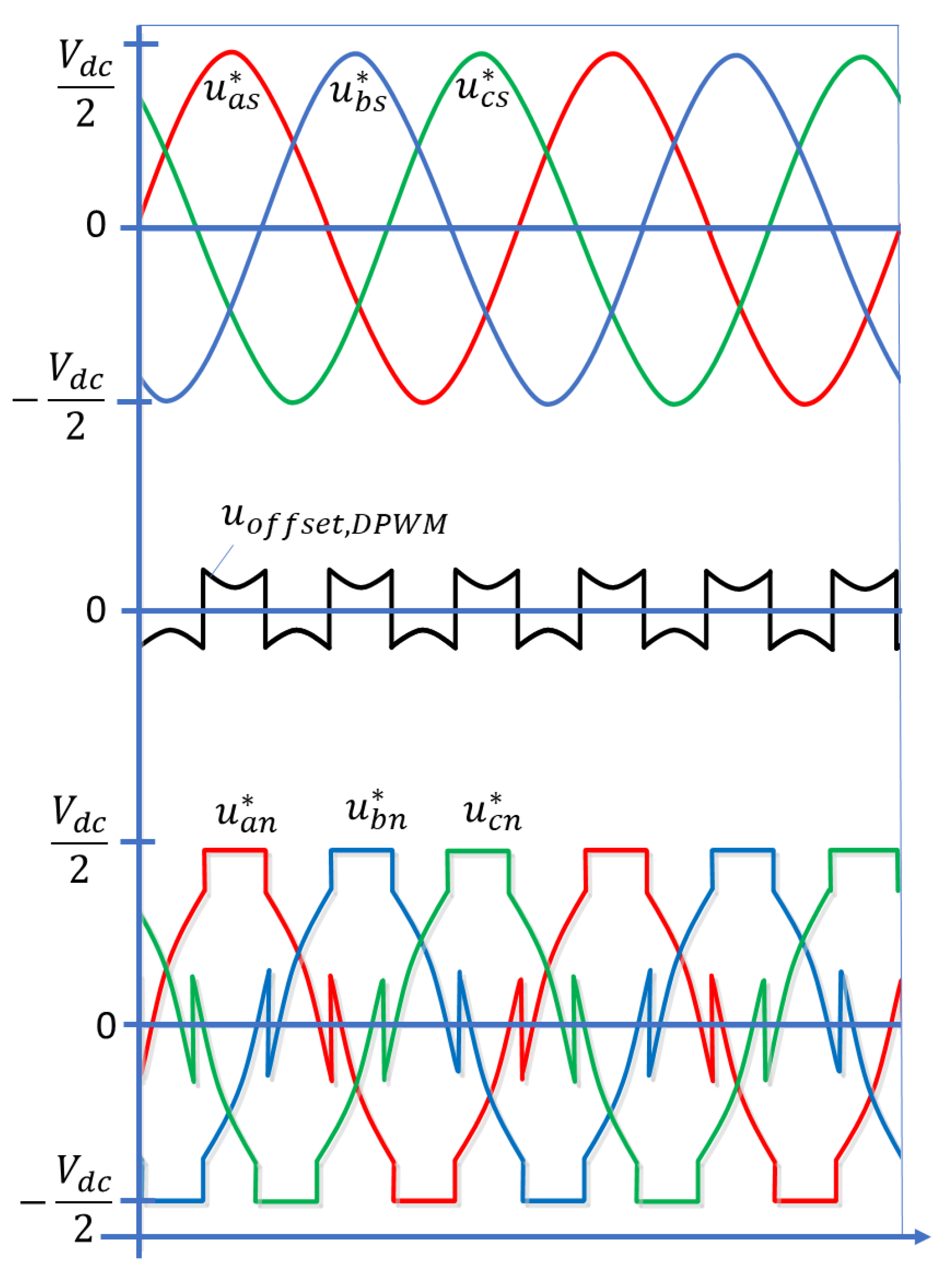Furthermore, it is known that by using DPWM, the switching losses are reduced, and better harmonic characteristics can be obtained for high modulation indices, compared with inverters that use continuous pulse-width modulation [23,24,25,26]. Although there are several different DPWM methods, conventional 60° DPWM is most commonly used for systems with the unity power factor. The idea behind the 60° DPWM method is schematically shown in Figure 5. Therefore, the pole reference voltages to be applied to the VSI are described by:

$$\begin{array}{l}{u}_{an}^{*}=u_{as}^{*}+u_{offset,DPWM}\\ u_{bn}^{*}=u_{bs}^{*}+u_{offset,DPWM}\\ u_{cn}^{*}=u_{cs}^{*}+u_{offset,DPWM}\end{array}$$

(18)

where u*_an, u*_bn, and u*_cn are the pole reference voltages to be applied to the VSI, whereas u*_as, u*_bs, and u*_cs are the optimal reference voltages by deadbeat DSVM-MPC of each phase, respectively. The voltage u_offset,DPWM is the offset voltage used in the DPWM, which is calculated as follows:

$$\{\begin{array}{cc}{u}_{offset,DPWM}=\frac{V_{dc}}{2}-u_{\max },& \left(u_{\max }+u_{\min }>0\right)\\ u_{offset,DPWM}=-\frac{V_{dc}}{2}-u_{\min },& \left(u_{\max }+u_{\min }<0\right)\end{array}$$

(19)

where u_max and u_min are, respectively, the maximum and the minimum values among the phase reference voltages.

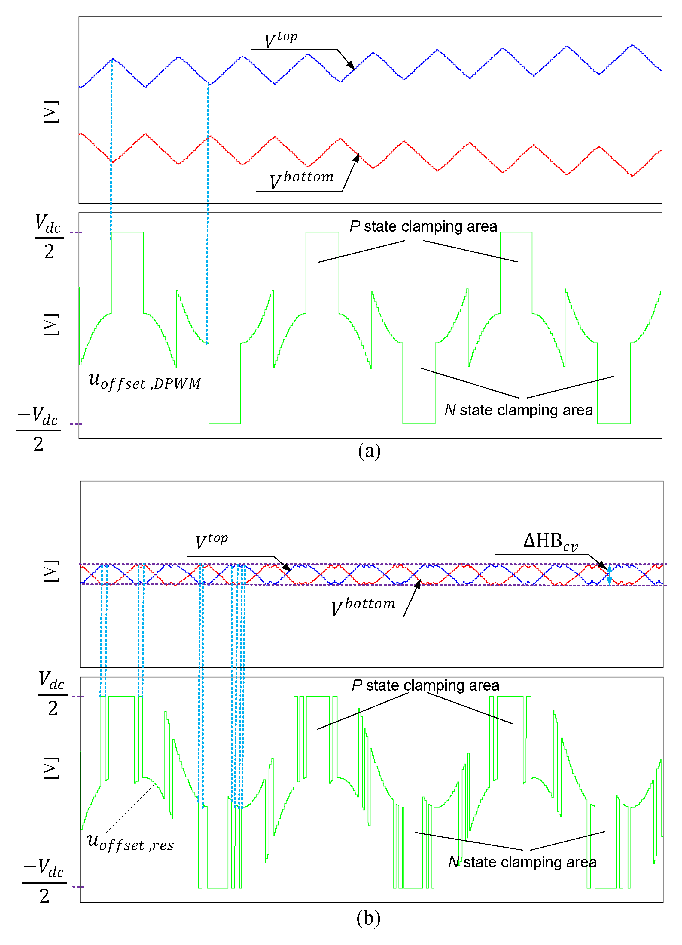
Figure 6a depicts the imbalance of the DC link capacitor voltage for the 3L T-type VSI. Note that when the switch of the either phase is locked in the P state, the top DC link capacitor voltage V^top is decreased and the bottom DC link capacitor voltage V^bottom is increased. Conversely, if the switch of the same switch is locked in the N state, the top and the bottom DC link capacitor voltages are increased and decreased, respectively. Thus, clamping plays a major role in decreasing or increasing the top and bottom capacitance voltages. Figure 6b shows the proposed DPWM method using the hysteresis capacitance voltage band ($\mathsf{\Delta }H{B}_{cv}$). The proposed neutral-point voltage balancing method uses a compensated voltage offset (u_offset,cv) depending on the top and bottom capacitor voltages in the linear modulation range. The u_offset,cv has an opposite influence from u_offset,DPWM on changing the direction of the top and bottom voltages, which is given as:

$$\{\begin{array}{cc}\begin{array}{l}{u}_{offset,\mathrm{cv}}=\frac{V_{dc}}{2}-u_{\max },\\ u_{offset,\mathrm{cv}}=-\frac{V_{dc}}{2}-u_{\min },\end{array}& \begin{array}{l}(V^{top}>V^{bottom})\\ (V^{top}<V^{bottom})\end{array}\end{array}.$$

(20)

The proposed method seeks to maintain the advantage of diminishing the stress on transistors and minimizing the power loss, while simultaneously achieving a balanced DC link capacitance voltage with a stable and acceptable capacitance voltage error $\left|E_{cv}\right|$, which is defined as

$$\left|E_{cv}\right|=\left|V^{top}-V^{bottom}\right|.$$

(21)

The capacitance voltage error $\left|E_{cv}\right|$ is inevitable; thus, it should be limited to an acceptable error band $\mathsf{\Delta }H{B}_{cv}$, to avoid large deviations of the DC link capacitance voltage and high switching. The limited error band is defined as $\left|E_{limit}\right|$. The resultant voltage offset (u_offset,res) can then be designed depending on the following condition:

$$\{\begin{array}{ll}{u}_{offset,res}=u_{offset,DPWM}+u_{offset,cv},& \left(\left|E_{cv}\right|>\left|E_{\lim it}\right|\right)\\ u_{offset,res}=u_{offset,DPWM},& \left(\left|E_{cv}\right|\le \left|E_{\lim it}\right|\right)\end{array}.$$

(22)

According to Equation (22), if the capacitance voltage error $\left|E_{cv}\right|$ exceeds the limited error band, the u_offset,cv will be injected into the u_offset,DPWM to have an opposite effect on the clamped voltage, otherwise, the u_offset,DPWM will continue with its normal operation.

The effect of the resultant voltage offset u_offset,res on one of the pole reference voltages to be applied to the VSI is seen in Figure 6b. Note that the clamping areas are almost similar to the conventional DPWM; at the same time, the error of the DC link capacitance voltage is stable. In addition, there is a short clamping area injected by the u_offset,cv to maintain the capacitance error range. It is noteworthy that the switching frequency of u_offset,res and the non-switching area depend mainly on the setting of $\left|E_{\mathrm{limit}}\right|$; increasing the limited error band will result in a lower switching of u_offset,res and will deteriorate the quality of the current, whereas reducing the limited error band will cause undesirable switching frequency of u_offset,res and a small clamping area. Thus, it is recommended that the tradeoff error band limit for achieving desirable current control performance be determined.

5. Simulation Results

Simulations using the PSIM software tool were conducted to validate the proposed method. The system configuration was similar to that shown in Figure 1. The DC link voltage (V_dc) was 300 V, and was distributed equally between the top capacitance voltage (V^top) and the bottom capacitance voltage (V^bottom). The total DC link capacitance was 2200 µF and the switching frequency was 10 kHz. The value of $\left|E_{limit}\right|$ was set empirically at 2.6 V. The simulation parameters are given in

Table 2. System parameters.

Variable	Description	Value	Unit
Pr	Rated power	2.1	kW
Vdc	DC link voltage	300	V
f	Fundamental frequency	60	Hz
e	Grid voltage	100	Vrms
Ts	Sampling time	100	$\mu s$
R	Load resistance	1	ohm
L	Filter inductance	2	mH
M	Modulation index	0.954

. After synthesizing the reference voltage vectors with the minimized cost function using the deadbeat DSVM-MPC system, the reference voltage vector was applied to the grid-connected 3L T-type VSI.

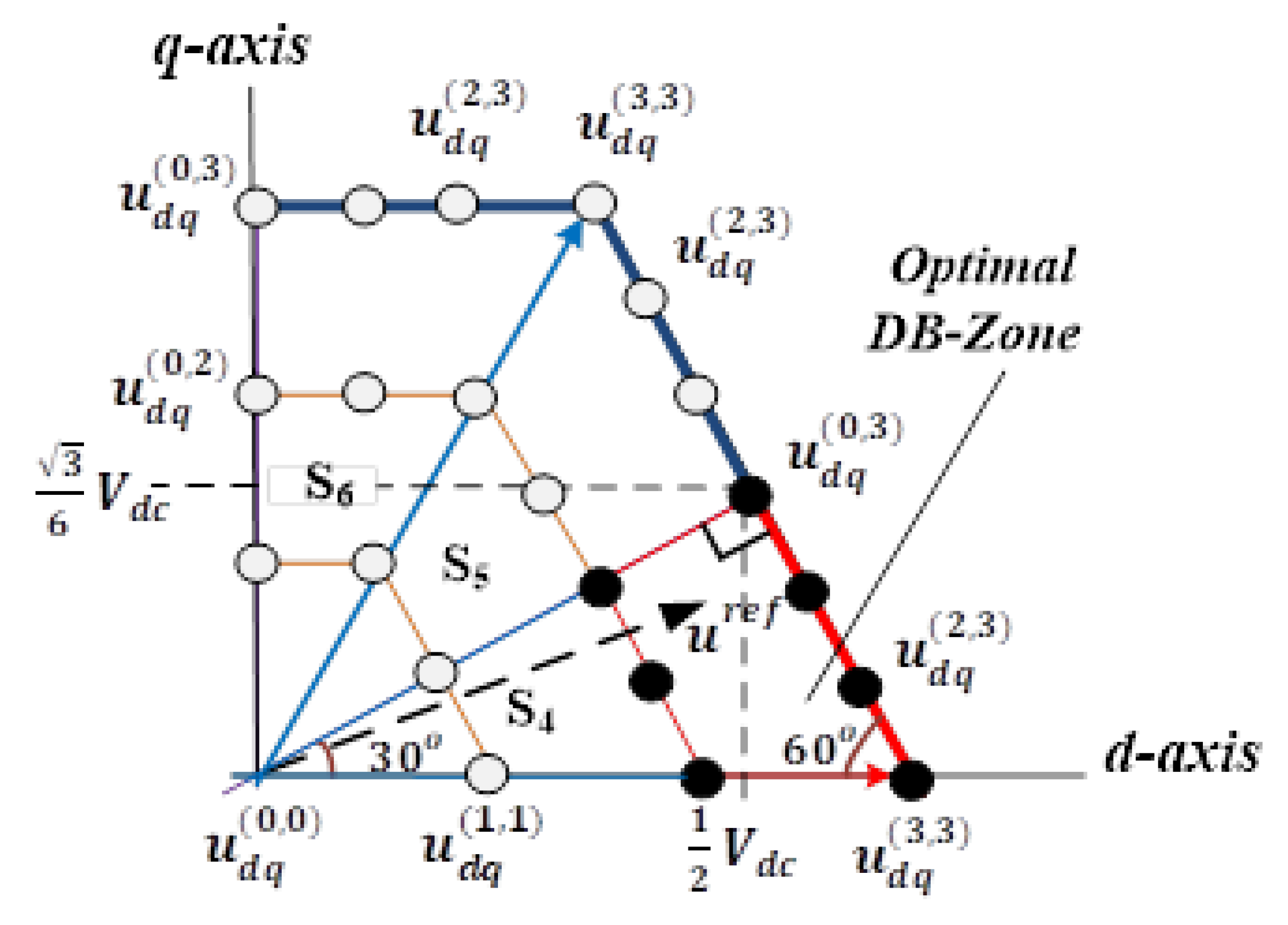
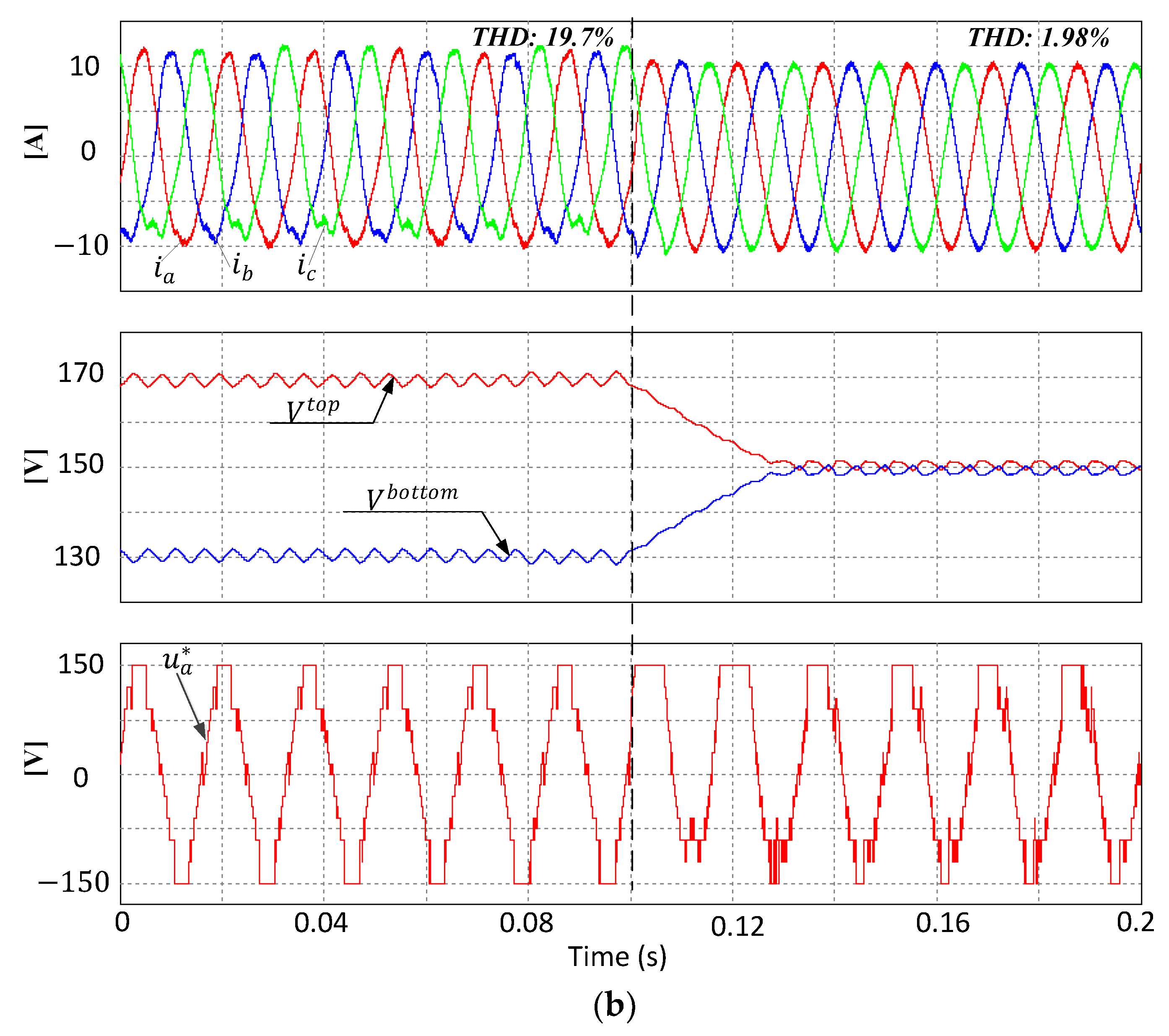
Figure 7 shows the simulation results for the optimal voltage vectors in the d–q frame for the deadbeat DSVM-MPC, which followed the reference current using only four candidate voltage vectors [20]. Figure 8 shows the simulation results for the deadbeat DSVM-MPC using the balancing method in Reference [20] and using the proposed DPWM method. It can be seen that the current waveforms became highly distorted before implementation of the neutral-point balancing of capacitance voltage, owing to large voltage deviations. Obviously, the total harmonic distortion (THD was is significantly reduced using either one of the balancing methods. Nevertheless, the proposed balancing method performed better in terms of THD, as shown in Figure 8b.

Figure 9 shows the simulation results for dynamic response for the deadbeat DSVM-MPC system, using the two balancing methods. As can be seen, both methods exhibited a fast dynamic current response, because the MPC method was used. On the other hand, the proposed method exhibited smaller THD compared with the method in Reference [20].

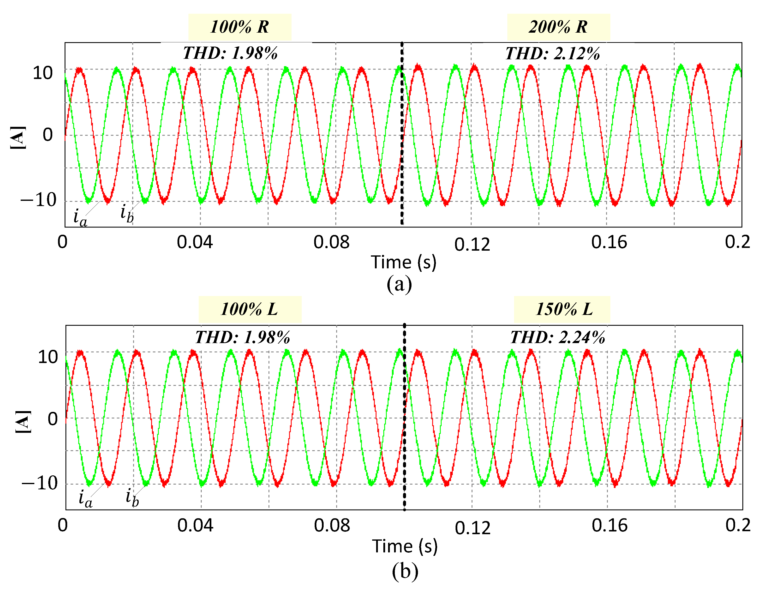
The robustness of the proposed method was shown by varying the impedances of the grid connected system including the inductance (L) and resistance (R) (Figure 10). The values of resistance and inductance were increased (at t = 0.1 s) by 100% and 50% of the nominal values, respectively. It can be obviously seen that there was a negligible increase in the THD. Therefore, it was confirmed that the proposed balancing method in FS-MPC with DSVM and DBC is robust to the variations of impedances.

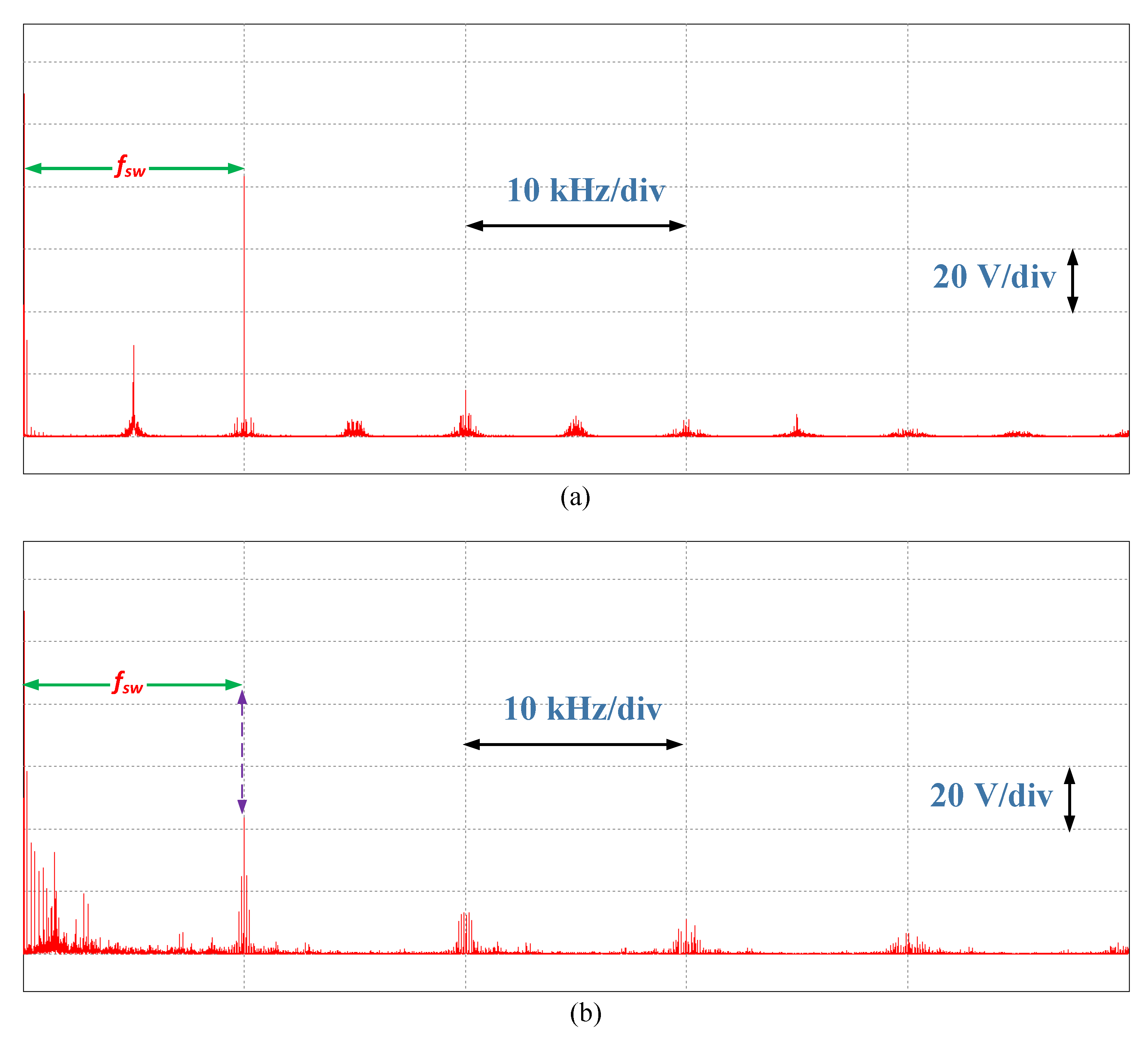
Figure 11a,b depicts the frequency spectrum of the phase voltage for the conventional method and proposed method, respectively. Apparently, the first harmonic component (i.e., switching frequency (f_sw)) was greatly reduced with the proposed algorithm, compared to the conventional method. This indicates the proposed method has less switching frequency owing to the use of the DPWM modulator, as mentioned previously.

6. Experimental Results

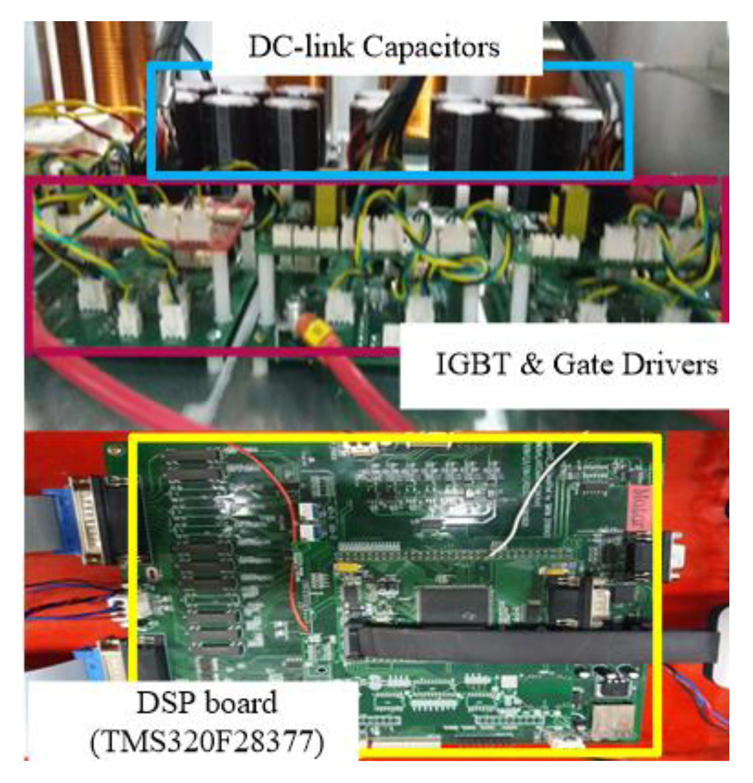
The proposed control system was further validated on a prototype grid-connected VSI that was used in a laboratory setup, as shown in Figure 12. The experimental parameters of the prototype were similar to those that were assumed in the simulation study, as shown in Table 2. The control system was configured using a DSP named TMS320F28377. In addition, 10-FZ12NMA080SH01-M260F-3 from Vincotech was employed to configure the three-level inverter system. To ensure a fair comparison of these methods, the experimental conditions were the same as those that were assumed in the simulation study. Thus, the limited error band $\left|E_{limit}\right|$ was also set at 2.6 V, which was similar to that in the simulation. To verify the effectiveness of the proposed method in the deadbeat DSVM-MPC, it was compared against the conventional neutral-point balancing method [20].

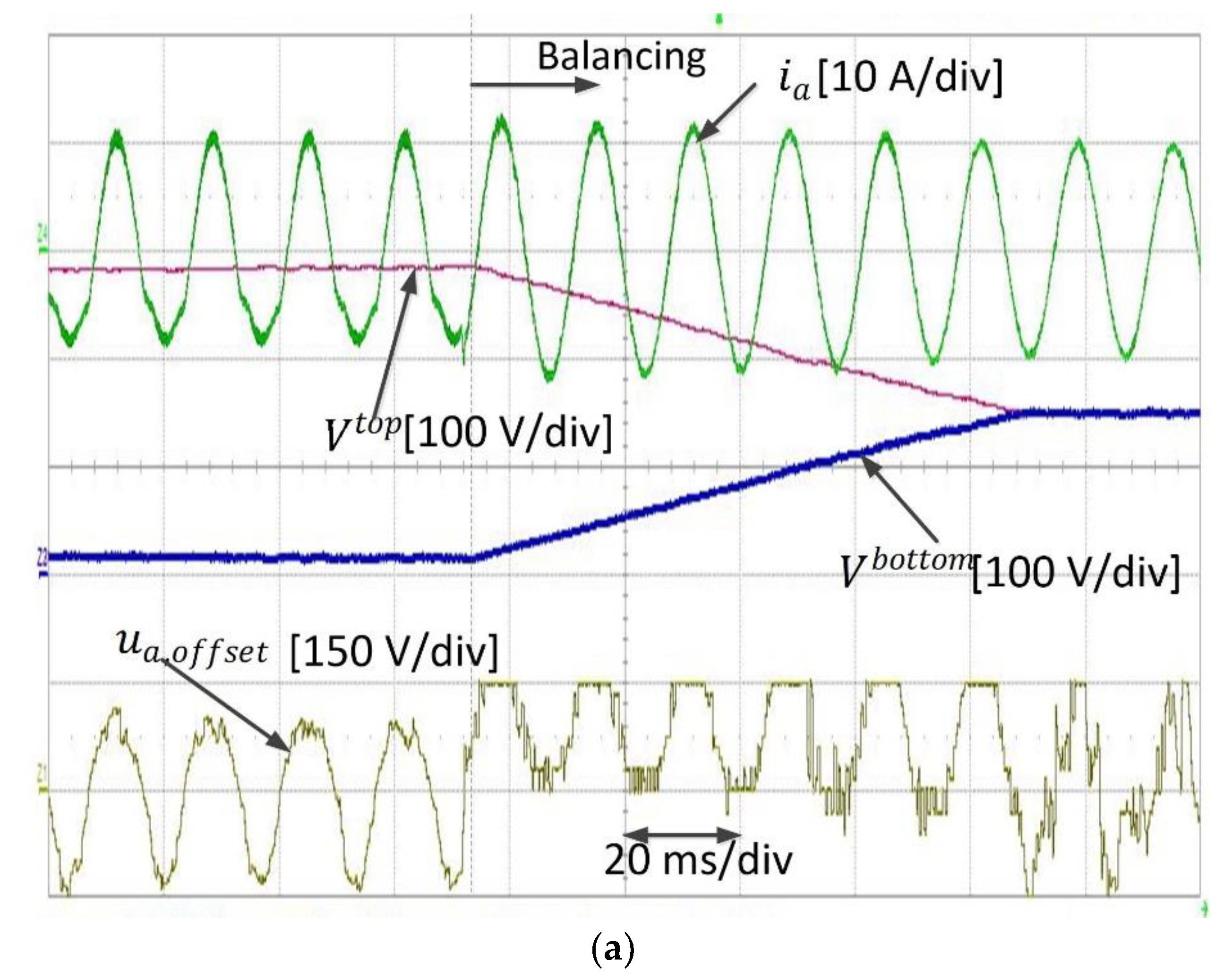
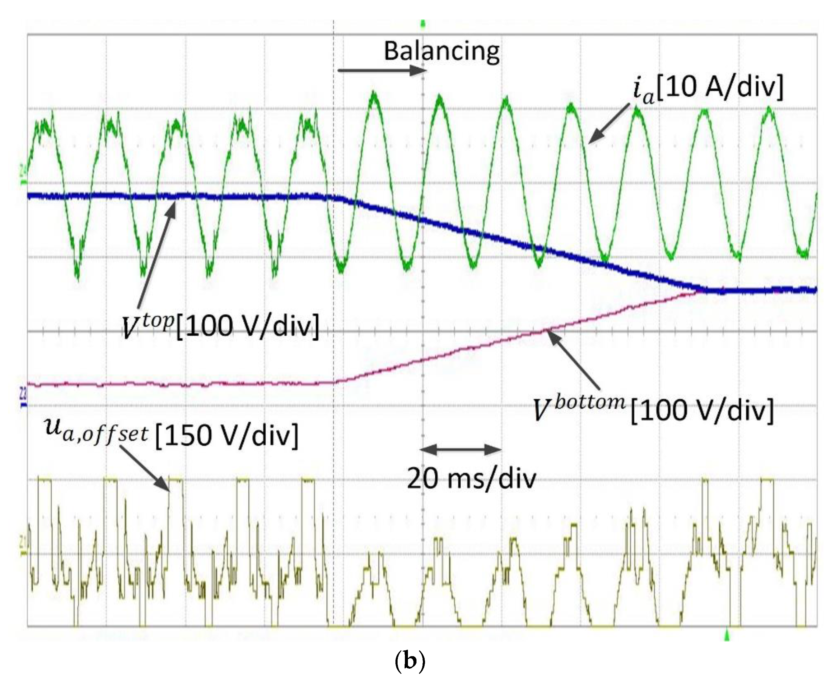
Figure 13 shows the experimental results for the grid current of the deadbeat DSVM-MPC, for both balancing methods. Similarly to the simulation results, it was observed that the proposed balancing method demonstrated a good capability of balancing the deviation of the top and bottom capacitance voltages. As can be seen, before applying either of the balancing methods, the difference between the top and bottom capacitor voltages was very high, and the output current became distorted owing to the neutral-point voltage imbalance. However, when the neutral-point voltage was balanced, the distortion of the output current disappeared. 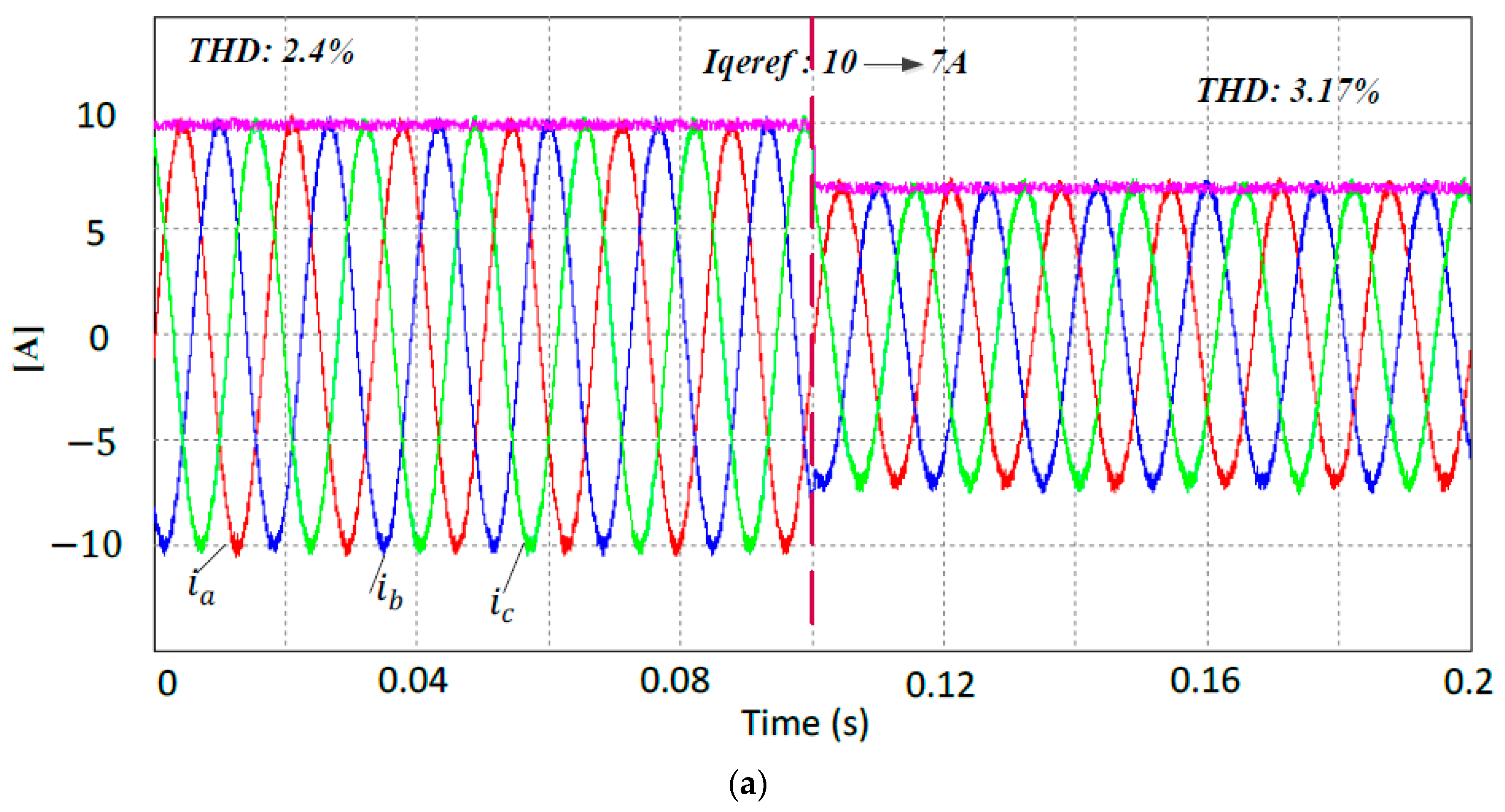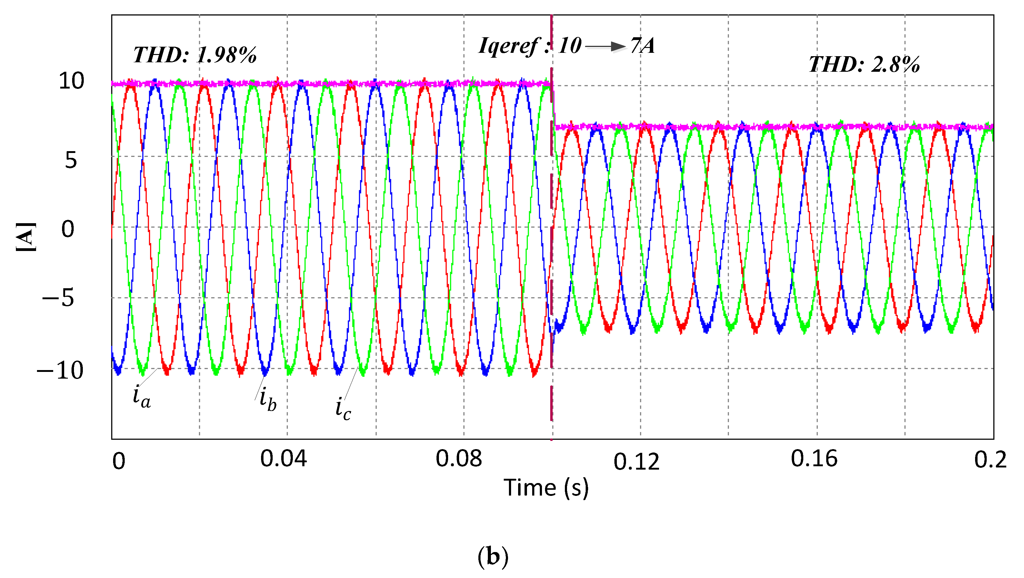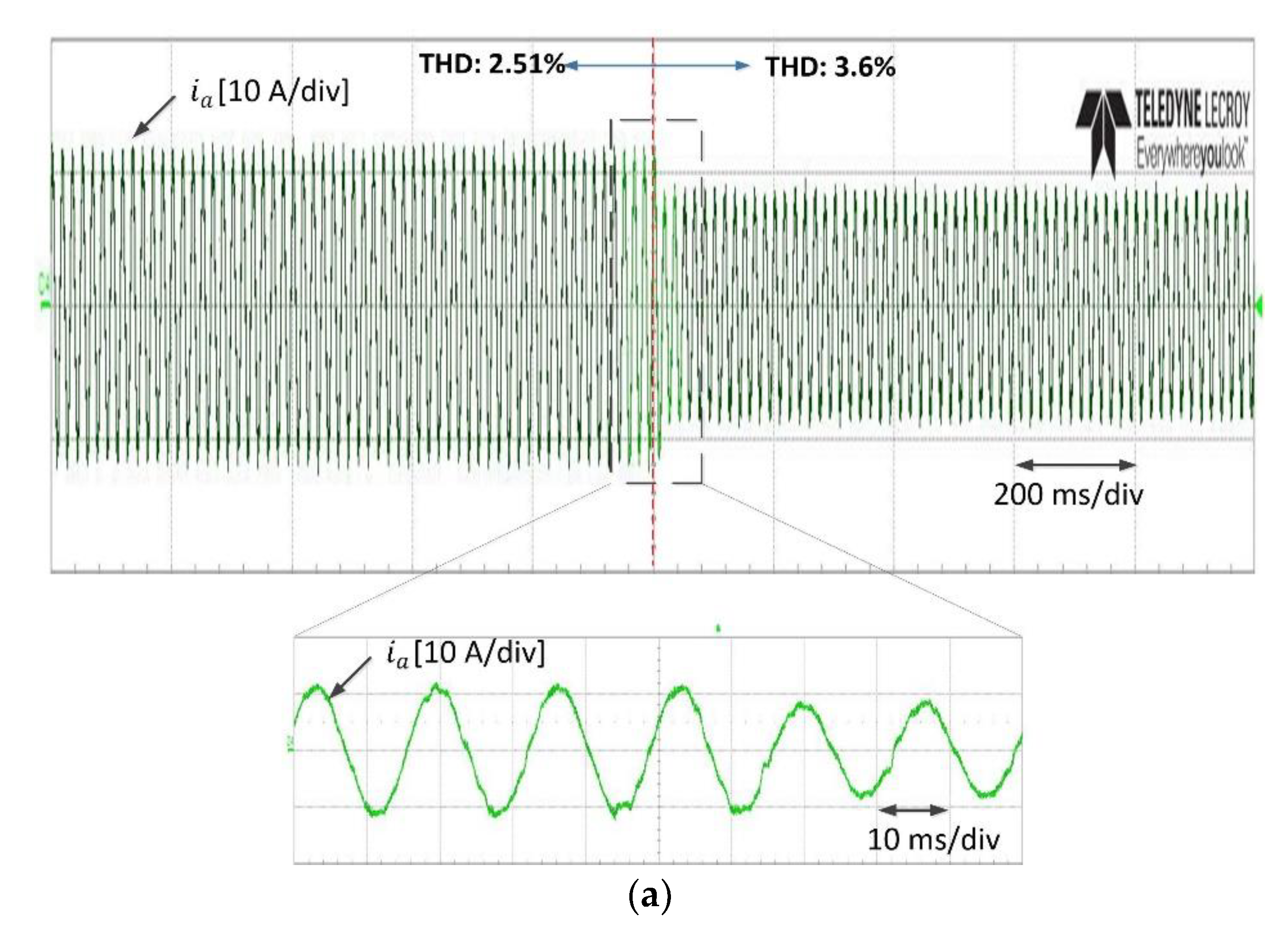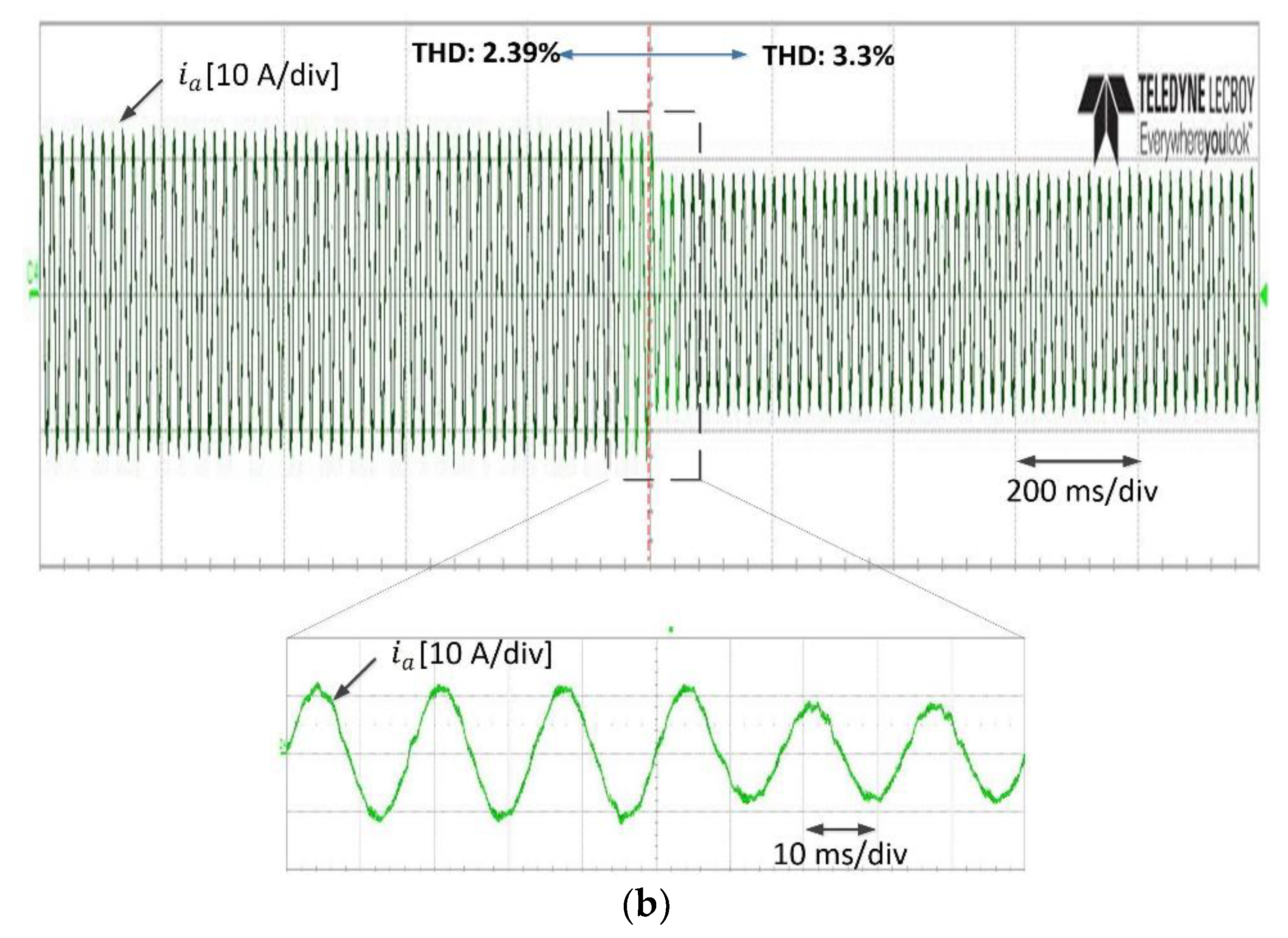Figure 14 shows the experimental results for the dynamic current performance from 10 A to 7 A for the deadbeat DSVM-MPC system, using both the conventional and the proposed balancing methods. As can be seen, the settling time was very short because the MPC method was used. However, the proposed balancing method exhibited lower THD by around 4.9% before and after the current reference change, when compared with the conventional neutral-point balancing method [20].

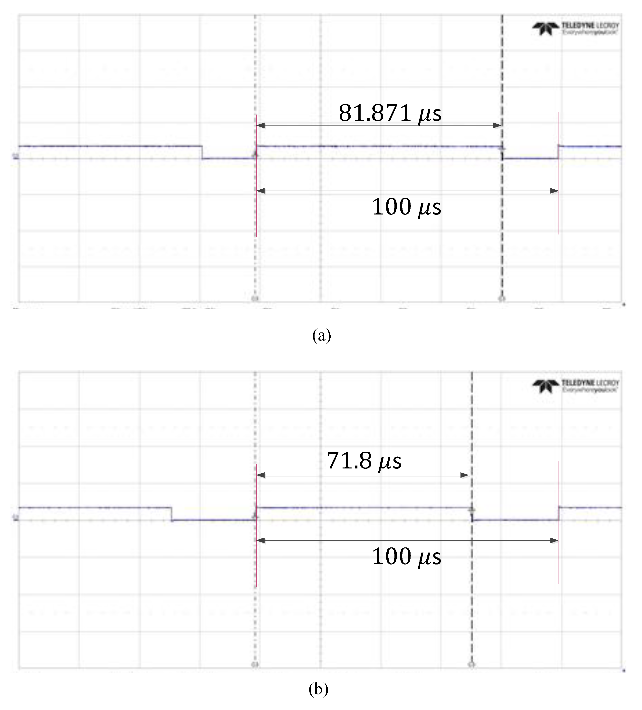
Figure 15 shows the comparison of the hardware computation time of the deadbeat DSVM-MPC system, without weighting factors, for the control method in Reference [20] and the proposed method. As can be seen, the computation time required by the proposed deadbeat DSVM-MPC method was reduced by 12.30% when compared to the method from Reference [20]. This indicates the simplicity of the proposed algorithm.

7. Conclusions

This paper proposed a deadbeat DSVM-MPC with a simplified neutral-point balancing method for enhancement of the output current quality in three-level grid-connected voltage source inverters. The DSVM-MPC method produces various virtual voltage vectors by subdividing the space vector diagram, and selects the optimal voltage vector that minimizes the error with respect to the reference current. To alleviate the computational burden, a deadbeat control was applied to restrict the optimal region of candidate voltage vectors. In addition, this work introduced simplified neutral-point capacitance voltage balancing using a modified DPWM method without a need for an extra cost function, thus reducing the total computation time. The reduction in the computation time may be advantageous for incorporating additional estimation or protection algorithms. The modified DPWM method had a higher efficiency than the conventional CPWM method, owing to the reduced number of switching operations.

References

1. Ma, W.; Sun, P.; Zhou, G.; Sailijiang, G.; Zhang, Z.; Liu, Y. A Low-Computation Indirect Model Predictive Control for Modular Multilevel Converters. J. Power Electron. 2019, 19, 529–539. [Google Scholar]
2. Rodriguez, J.; Kazmierkowski, M.P.; Espinoza, J.R.; Zanchetta, P.; Abu-Rub, H.; Young, H.A.; Rojas, C.A. State of the art of finite control set model predictive control in power electronics. IEEE Trans. Ind. Inform. 2013, 9, 1003–1016. [Google Scholar] [CrossRef]
3. Alsofyani, I.M.; Kim, S.; Lee, K. Finite Set Predictive Torque Control Based on Sub-divided Voltage Vectors of PMSM with Deadbeat Control and Discrete Space Vector Modulation. In Proceedings of the 2019 IEEE Applied Power Electronics Conference and Exposition (APEC), Anaheim, CA, USA, 17–21 March 2019; pp. 1853–1857. [Google Scholar]
4. Zhao, B.; Li, H.; Mao, J. Double-Objective Finite Control Set Model-Free Predictive Control with DSVM for PMSM Drives. J. Power Electron. 2019, 19, 168–178. [Google Scholar]
5. El-naggar, M.F.; Elgammal, A.A.A. Multi-Objective Optimal Predictive Energy Management Control of Grid-Connected Residential Wind-PV-FC-Battery Powered Charging Station for Plug-in Electric Vehicle. J. Electr. Eng. Technol. 2018, 13, 742–751. [Google Scholar]
6. Kwak, S.; Moon, U.-C.; Park, J.-C. Predictive-control-based direct power control with an adaptive parameter identification technique for improved AFE performance. IEEE Trans. Power Electron. 2014, 29, 6178–6187. [Google Scholar] [CrossRef]
7. Cortes, P.; Rodriguez, J.; Vazquez, S.; Franquelo, L.G. Predictive control of a three-phase UPS inverter using two steps prediction horizon. In Proceedings of the 2010 IEEE International Conference on Industrial Technology, Vina del Mar, Chile, 14–17 March 2010; pp. 1283–1288. [Google Scholar]
8. Vazquez, S.; Montero, C.; Bordons, C.; Franquelo, L.G. Design and experimental validation of a model predictive control strategy for a VSI with long prediction horizon. In Proceedings of the IECON 2013-39th Annual Conference of the IEEE Industrial Electronics Society, Vienna, Austria, 10–13 November 2013; pp. 5788–5793. [Google Scholar]
9. Karamanakos, P.; Geyer, T.; Oikonomou, N.; Kieferndorf, F.D.; Manias, S. Direct model predictive control: A review of strategies that achieve long prediction intervals for power electronics. IEEE Ind. Electron. Mag. 2014, 8, 32–43. [Google Scholar] [CrossRef]
10. Xie, W.; Wang, X.; Wang, F.; Xu, W.; Kennel, R.M.; Gerling, D.; Lorenz, R.D. Finite-control-set model predictive torque control with a deadbeat solution for PMSM drives. IEEE Trans. Ind. Electron. 2015, 62, 5402–5410. [Google Scholar] [CrossRef]
11. Park, J.Y.; Sin, J.; Bak, Y.; Park, S.-M.; Lee, K.-B. Common-mode Voltage Reduction for Inverters Connected in Parallel Using an MPC Method with Subdivided Voltage Vectors. J. Electr. Eng. Technol. 2018, 13, 1212–1222. [Google Scholar]
12. Vazquez, S.; Leon, J.I.; Franquelo, L.G.; Carrasco, J.M.; Martinez, O.; Rodriguez, J.; Cortes, P.; Kouro, S. Model predictive control with constant switching frequency using a discrete space vector modulation with virtual state vectors. In Proceedings of the 2009 IEEE International Conference on Industrial Technology, Gippsland, Australia, 10–13 February 2009. [Google Scholar]
13. Wang, Y.; Wang, X.; Xie, W.; Wang, F.; Dou, M.; Kennel, R.M.; Lorenz, R.D.; Gerling, D. Deadbeat model-predictive torque control with discrete space-vector modulation for PMSM drives. IEEE Trans. Ind. Electron. 2017, 64, 3537–3547. [Google Scholar] [CrossRef]
14. Kouro, S.; Cortes, P.; Vargas, R.; Ammann, U.; Rodriguez, J. Model predictive control—A simple and powerful method to control power converters. IEEE Trans. Ind. Electron. 2009, 56, 1826–1838. [Google Scholar] [CrossRef]
15. Li, J.; Chang, X.; Yang, D.; Liu, Y.; Jiang, J. Deadbeat and Hierarchical Predictive Control with Space-Vector Modulation for Three-Phase Five-Level Nested Neutral Point Piloted Converters. J. Power Electron. 2018, 18, 1791–1804. [Google Scholar]
16. Wang, C.; Li, Y. Analysis and calculation of zero-sequence voltage considering neutral-point potential balancing in three-level NPC converters. IEEE Trans. Ind. Electron. 2010, 57, 2262–2271. [Google Scholar] [CrossRef]
17. Lee, J.-S.; Lee, K.-B. Time-offset injection method for neutral-point AC ripple voltage reduction in a three-level inverter. IEEE Trans. Power Electron. 2016, 31, 1931–1941. [Google Scholar] [CrossRef]
18. Moon, H.-C.; Lee, J.-S.; Lee, J.-H.; Lee, K.-B. MPC-SVM method with subdivision strategy for current ripples reduction and neutral-point voltage balance in three-level inverter. In Proceedings of the 2017 IEEE Energy Conversion Congress and Exposition (ECCE), Cincinnati, OH, USA, 1–5 October 2017; pp. 191–196. [Google Scholar]
19. Wang, C.; Li, Z.; Xin, H. Neutral-point Voltage Balancing Strategy for Three-level Converter based on Disassembly of Zero Level. J. Power Electron. 2019, 19, 79–88. [Google Scholar]
20. Lee, J.; Lee, J.; Moon, H.; Lee, K. An Improved Finite-Set Model Predictive Control Based on Discrete Space Vector Modulation Methods for Grid-Connected Three-Level Voltage Source Inverter. IEEE J. Emerg. Sel. Top. Power Electron. 2018, 6, 1744–1760. [Google Scholar] [CrossRef]
21. Shueai Alnamer, S.; Mekhilef, S.; Bin Mokhlis, H. A Four-Level T-Type Neutral Point Piloted Inverter for Solar Energy Applications. Energies 2018, 11, 1546. [Google Scholar] [CrossRef]
22. Choi, U.M.; Lee, H.H.; Lee, K.B. Simple neutral-point voltage control for three-level inverters using a discontinuous pulse width modulation. IEEE Trans. Energy Convers. 2013, 28, 434–443. [Google Scholar] [CrossRef]
23. Tcai, A.; Alsofyani, I.M.; Seo, I.-Y.; Lee, K.-B. DC-link Ripple Reduction in a DPWM-Based Two-Level VSI. Energies 2018, 11, 3008. [Google Scholar] [CrossRef]
24. Tcai, A.; Alsofyani, I.M.; Lee, K. DC-link Ripple Reduction in a DPWM-based Two-Level VSC. In Proceedings of the IEEE Energy Conversion Congress and Exposition (ECCE), Portland, OR, USA; 2018; pp. 1483–1487. [Google Scholar]
25. Lee, K.-B.; Lee, J.-S. Reliability Improvement Technology for Power Converters; Springer: Singapore, 2017. [Google Scholar]
26. Wang, X.; Zhao, J.; Wang, Q.; Li, G.; Zhang, M. Fast FCS-MPC-Based SVPWM Method to Reduce Switching States of Multilevel Cascaded H-Bridge STATCOMs. J. Power Electron. 2019, 19, 244–253. [Google Scholar]
Figure 1. Circuit diagram of three-level T-type inverter.
Energies 12 03111 g001
Figure 2. Space vector diagram of conventional finite-set model predictive control (FS-MPC).
Energies 12 03111 g002
Figure 3. Space vector diagram of conventional model predictive control with discrete space vector modulation (DSVM-MPC).
Energies 12 03111 g003
Figure 4. Space vector diagram of conventional DSVM-MPC.
Energies 12 03111 g004
Figure 5. Reference voltage, offset voltage, and pole reference voltages of the conventional 60° discontinuous pulse-width modulation (DPWM).
Energies 12 03111 g005
Figure 6. Behavior of top and bottom capacitance voltages with respect to: (a) conventional DPWM; (b) proposed DPWM.
Energies 12 03111 g006
Figure 7. Simulation results of the optimal voltage vectors for the deadbeat FS-MPC with DSVM.
Energies 12 03111 g007
Figure 8. Simulation results of capacitance voltage balancing for deadbeat DSVM-MPC. (a) Conventional balancing method [20]. (b) Proposed balancing method.
Energies 12 03111 g008aEnergies 12 03111 g008b
Figure 9. Simulation results of current dynamic response for deadbeat DSVM-MPC with (a) conventional balancing method [20] and (b) proposed balancing method.
Energies 12 03111 g009aEnergies 12 03111 g009b
Figure 10. Simulation results of grid impedance variation for the proposed method.
Energies 12 03111 g010
Figure 11. Simulation results of frequency spectrum for the phase voltage with (a) conventional balancing method [20] and (b) proposed balancing method.
Energies 12 03111 g011
Figure 12. Experimental setup.
Energies 12 03111 g012
Figure 13. Experimental results of capacitance voltage balancing for deadbeat DSVM-MPC. (a) Conventional balancing method [20]. (b) Proposed balancing method.
Energies 12 03111 g013aEnergies 12 03111 g013b
Figure 14. Experimental results of current dynamic response for deadbeat DSVM-MPC for the (a) conventional balancing method [20] and (b) proposed balancing method.
Energies 12 03111 g014aEnergies 12 03111 g014b
Figure 15. The hardware execution time. (a) Deadbeat FS-MPC with extra cost function [20]. (b) Proposed method.
Energies 12 03111 g015