Long-Term Demand Forecasting in a Scenario of Energy Transition

Abstract

The energy transition from fossil fuels to carbon-free sources will be a big challenge in the coming decades. In this context, the long-term prediction of energy demand plays a key role in planning energy infrastructures and in adopting economic and energy policies. In this article, we aimed to forecast energy demand for Spain, mainly employing econometrics techniques. From information obtained from institutional databases, energy demand was decomposed into many factors and economy-related activity sectors, obtaining a set of disaggregated sequences of time-dependent values. Using time-series techniques, a long-term prediction was then obtained for each component. Finally, every element was aggregated to obtain the final long-term energy demand forecast. For the year 2030, an energy demand equivalent to 82 million tons of oil was forecast. Due to improvements in energy efficiency in the post-crisis period, a decoupling of economy and energy demand was obtained, with a 30% decrease in energy intensity for the period 2005–2030. World future scenarios show a significant increase in energy demand due to human development of less developed economies. For Spain, our research concluded that energy demand will remain stable in the next decade, despite the foreseen 2% annual growth of the nation’s economy. Despite the enormous energy concentration and density of fossil fuels, it will not be affordable to use them to supply energy demand in the future. The consolidation of renewable energies and increasing energy efficiency is the only way to satisfy the planet’s energy needs.

1. Introduction

Modern societies face the challenge of transitioning to a new energy model that permits continuing fulfilment of increasing energy demand while meeting the requirements presented for climate change and sustainability, which can be summarized in the so-called energy trilemma [1] depicted in Figure 1. Industry and governments have to simultaneously pursue energy security (reliability of energy infrastructure, and ability of energy providers to meet current and future demand), energy equity (accessibility and affordability of energy supply across the population), and environmental sustainability (energy efficiency and the development of energy supplies from renewable and other low-carbon sources).

The commitments of the European Union, derived from the Paris Agreement, established a goal of reducing emissions between 80% and 95% by 2050, compared to 1990 levels [2]. This necessarily leads to the electrification of most of the energy demand, which would cause the demand for electricity to approximately double what it is currently before the year 2060 [3].

In this context, the prediction of energy demand plays a key role in planning energy infrastructures and in adopting economic and energy policies. Besides institutional and national studies, many academic works have addressed this problem, adopting global [4], regional [5], national [6,7], or even local [8] perspectives.

Energy forecasting has been addressed in the literature, mainly considering three different prediction horizons: short-term (an hour to a week) [9,10], mid-term (a month to 5 years) [11], and long-term (5 to 20 years) [12]. Prediction methods can be additionally categorized into two types: data-driven methods, where the relationship between the energy demand and its causal variables is automatically discovered using statistical procedures [13]; and model-driven, where this relationship has been previously established [14].

Data-driven methods can be classified as autoregressive (those using only historical data to make predictions) and causal (those which also consider external variables influencing energy demand, such as temperature, economy, etc.).

Once the variables used to make predictions (either only past values or past and external values) have been established, different data-driven forecasting techniques have also been suggested in the literature, such as artificial neural networks [10], fuzzy logic [15], time-series analysis [16], regression models [6], support vector machines [17], or genetic algorithms [18].

By contrast, model-driven predictions can be made using system dynamics [19], or, more often, econometric models [20,21]. For large horizons (long-term predictions), data-driven methods are more likely to fail, as the forecasting error usually increases with the length of the prediction horizon. Thus, econometric models are the most commonly employed technique [22]. Ghalehkhondabi et al. [23] have made an overview of general energy demand forecasting methods.

Econometric models have been employed to forecast energy demand for regions as diverse as, for instance, China [24], South Korea [25], Mexico [26], United Kingdom [27], South Africa [28], United States [29], or Europe [30].

Some other works have also addressed long-term energy demand prediction for Spain, as it is an active country in the renewable energy market [31]. Most of them have addressed partial aspects [32,33,34,35,36,37], although research from a more general perspective can be found in References [38,39]. However, these two general approaches focus only on electricity demand and not overall energy consumption, which is the key factor determining CO₂ emissions.

In our research, the goal was to obtain a long-term forecast (year 2030) of the Spanish total energy demand. As was suggested by the literature review described in the previous paragraphs, the approach of this paper used econometrics techniques. From information obtained in institutional databases, energy demand was decomposed into many factors and economy-related activity sectors, obtaining a set of disaggregated sequences of time-dependent values. Using time-series techniques, a long-term prediction was then obtained for each component. Finally, every element was aggregated to obtain the final long-term energy demand forecast.

2. Materials and Methods

2.1. Data Sources

The data used in this paper can be found in the Eurostat (European Statistical Office) databases [40]. More specifically, for this research, population [41], economic [42], energy [43], and climate change [44] magnitudes were considered for Spain for the period 1990–2015.

The energy magnitudes have been disaggregated into $n=30$ activity sectors (level 1), as it is detailed in

Table 1. Sectors of activity considered for energy demand disaggregation.

Sector	Level 1	Level 2	Level 3
1	Agriculture and Forestry	A: Agriculture and Forestry	A: Agriculture and Forestry
2	Chemical and Petrochemical	I: Industry	I: Industry
3	Iron and Steel
4	Non-Metallic Minerals
5	Wood and Wood Products
6	Construction
7	Paper, Pulp and Print
8	Food and Tobacco
9	Textile and Leather
10	Machinery
11	Transport Equipment
12	Non-Specified (Industry)
13	Mining and Quarrying
14	Others (Industry)
15	Hotels, Restaurants	S: Services	S: Services
16	Health and Social Action Sector
17	Education, Research
18	Trade (Wholesale and Retail)
19	Public and Private Offices
20	Others (Services)
21	Cars	Tp: Passenger Transport	T: Transport
22	Buses
23	Rail Transport of Passengers
24	Others in Passenger Transport
25	Trucks and Light Vehicles	Tf: Freight Transport
26	Inland Waterways
27	Rail Transport of Goods
28	Others (Transport)	To: Others (Transport)
29	Occupied Dwellings	R: Residential	R: Residential
30	Others	O: Others	O: Others

.

Some medium (level 2) or coarse (level 3) partial disaggregation has also been employed in some representations through the article. The structure of energy demand disaggregation is depicted in Figure 2.

2.2. The Kaya Identity

In energy transition scenarios, the emission of the greenhouse gas carbon dioxide is one of the most relevant variables to be considered. For that reason, in the last decade of the 20th century, the Kaya identity [45] was proposed as a method to decompose the influence of different elements on CO₂ emissions. This identity can be formulated as:

$$C=P·G_p·I_e·F_e$$

(1)

where $C$ is the global CO₂ emissions due to human activities; $P$ is the world’s total population; $G_p$ is defined as $G/P$, that is, the world’s gross domestic product (GDP: $G$) per person ($P$); $I_e$ is the energy intensity, defined as $E/G$, with $E$ being the global energy consumption; and $F_e$ is the carbon footprint of energy, defined as $F/E$. Substituting these definitions into Equation (1), the Kaya identity can also be formulated as:

$$C=P·\frac{G}{P}·\frac{E}{G}·\frac{F}{E}$$

(2)

The increase of the population ($P$) and the development of the economy ($G_p$) are the main elements that identify the energy needs of a society. Following the Kaya identity, future increase of population and economic growth can be compensated through an improvement in energy efficiency (lower values of $I_e$) and the decarbonization of the energy consumed (lower values of $F_e$). The reduction of greenhouse gas emissions justifies actions aimed at reducing these two factors. In the context of this paper, aimed at energy demand forecasting, only the first three factors of the Kaya identity were considered, while the fourth ($F_e$) should play a key role in energy production policies.

2.3. Laspeyres Decomposition

Most of the member countries of the OECD (Organisation for Economic Co-operation and Development) have established energy saving and efficiency objectives in their energy and environmental policies. However, there is a big challenge in measuring these values and their progress over the time. The problem becomes even more complex if there are economic changes and, jointly, improvements in energy efficiency. To tackle this issue, several decomposition methods have been proposed [46]. By far the most employed techniques in energy studies are the Laspeyres method [47,48,49] and the logarithmic mean Divisia index (LMDI) [50,51], due to their ease of understanding and their advantages over other competing indices (Fischer [52] or Paasche [53]).

To obtain the energy demand forecast, the following procedure (as depicted in Figure 3) was employed:

• Using a decomposition method, the raw economic data (1990–2015) were disaggregated into several economic sectors and, for every sector, into three factors (activity, structure, and intensity), which will be defined below.
• The time-series obtained for every sector and factor was used to forecast its values (2030). The forecasted values were then aggregated to obtain a prediction of the energy demand.

Let us call $n$ the number of economic sectors of a certain economy. At a given time, $t$, we will use the following definitions:

• $A^{\left(i\right)}\left(t\right)$: level of activity of the $i$-th sector, which is measured by the gross value added for the industry and services sectors, by population for residential consumption, and by passenger-kilometers and ton-kilometers for the sectors of passenger and freight transport, respectively;
• $E^{\left(i\right)}\left(t\right)$: energy consumption of the $i$-th sector;
• $A\left(t\right)$: total level of activity, considering all the sectors;
• $S^{\left(i\right)}\left(t\right)=A^{\left(i\right)}\left(t\right)/A\left(t\right)$: weight of the $i$-th sector in the structure of the economy;
• $I^{\left(i\right)}\left(t\right)=E^{\left(i\right)}\left(t\right)/A^{\left(i\right)}\left(t\right)$: energy intensity of the $i$-th sector;

Based on these definitions, it can be written that:

$$E^{\left(i\right)}\left(t\right)=A\left(t\right)·\frac{A^{\left(i\right)}\left(t\right)}{A\left(t\right)}·\frac{E^{\left(i\right)}\left(t\right)}{A^{\left(i\right)}\left(t\right)}=A\left(t\right)·S^{\left(i\right)}\left(t\right)·I^{\left(i\right)}\left(t\right).$$

(3)

The change of energy consumption due to a change in the total level of activity for a period of time between $t_0$ and $T$ can be expressed, as shown in Appendix A, as:

$$\mathsf{\Delta }{E}_A^{\left(i\right)}=A\left(T\right)·S^{\left(i\right)}\left(t_0\right)·I^{\left(i\right)}\left(t_0\right)-E^{\left(i\right)}\left({\mathrm{t}}_0\right)+{\epsilon }_A^{\left(i\right)}.$$

(4)

Analogously, the other two components are defined as:

$$\begin{gathered} \mathsf{\Delta }{E}_S^{\left(i\right)}=A\left(t_0\right)·S^{\left(i\right)}\left(T\right)·I^{\left(i\right)}\left(t_0\right)-E^{\left(i\right)}\left({\mathrm{t}}_0\right)+{\epsilon }_S^{\left(i\right)}; \\ \mathsf{\Delta }{E}_I^{\left(i\right)}=A\left(t_0\right)·S^{\left(i\right)}\left(t_0\right)·I^{\left(i\right)}\left(T\right)-E^{\left(i\right)}\left({\mathrm{t}}_0\right)+{\epsilon }_I^{\left(i\right)}. \end{gathered}$$

(5)

Considering now the $\mathrm{n}$ sectors of the economy, we obtain:

$$\mathsf{\Delta }E=\sum _{i=1}^n\mathsf{\Delta }{E}^{\left(i\right)}=\sum _{i=1}^n\left(\mathsf{\Delta }{E}_A^{\left(i\right)}+\mathsf{\Delta }{E}_S^{\left(i\right)}+\mathsf{\Delta }{E}_I^{\left(i\right)}\right)=\sum _{i=1}^n\mathsf{\Delta }{E}_A^{\left(i\right)}+\sum _{i=1}^n\mathsf{\Delta }{E}_S^{\left(i\right)}+\sum _{i=1}^n\mathsf{\Delta }{E}_I^{\left(i\right)}.$$

(6)

For the activity component, it can be written, as shown in Appendix A, that:

$$\mathsf{\Delta }{E}_A=\left[{\mathrm{A}}_{\mathrm{T}}\sum _{i=1}^n{S}_0^{\left(i\right)}·I_0^{\left(i\right)}\right]-E_0+{\epsilon }_A.$$

(7)

Analogously, the other two components are:

$$\mathsf{\Delta }{E}_S=\left[{\mathrm{A}}_0\sum _{i=1}^n{S}_T^{\left(i\right)}·I_0^{\left(i\right)}\right]-E_0+{\epsilon }_S; \mathsf{\Delta }{E}_I=\left[{\mathrm{A}}_0\sum _{i=1}^n{S}_0^{\left(i\right)}·I_T^{\left(i\right)}\right]-E_0+{\epsilon }_I.$$

(8)

Finally, the increasing energy demand is decomposed as:

$$\mathsf{\Delta }E=\mathsf{\Delta }{E}_A+\mathsf{\Delta }{E}_S+\mathsf{\Delta }{E}_I.$$

(9)

This expression is called the additive decomposition. It is sometimes preferred to use the ratio of increasing energy demand, $R_E$, instead of the direct value of this increase ($\mathsf{\Delta }E$).

$$R_E\equiv \frac{E_T}{E_0}.$$

(10)

In the common case where $\mathsf{\Delta }{E}_A,\mathsf{\Delta }{E}_S,\mathsf{\Delta }{E}_I\ll E_0$, the increase of energy demand is multiplicatively decomposed, as shown in Appendix A, as:

$$R_E\approx R_{EA}·R_{ES}·R_{EI}=\frac{{\mathrm{A}}_{\mathrm{T}}{\sum }_{i=1}^n{S}_0^{\left(i\right)}·I_0^{\left(i\right)}}{E_0}·\frac{{\mathrm{A}}_0{\sum }_{i=1}^n{S}_T^{\left(i\right)}·I_0^{\left(i\right)}}{E_0}·\frac{{\mathrm{A}}_0{\sum }_{i=1}^n{S}_0^{\left(i\right)}·I_T^{\left(i\right)}}{E_0}+{\epsilon }^{\prime }.$$

(11)

2.4. LMDI Decomposition

In logarithmic mean Divisia index (LMDI) decomposition, the change of energy consumption due to a change in the total level of activity, for a period of time between $t_0$ and $T$, can be expressed, as detailed in Appendix B, as:

$$\mathsf{\Delta }{E}_A^{\left(i\right)}\equiv E_A^{\left(i\right)}\left(T\right)-E_A^{\left(i\right)}\left(t_0\right)=E^{\left(i\right)}\left(t^{*}\right)·\left\{Ln\left[A^{\left(i\right)}\left(T\right)\right]-Ln\left[A^{\left(i\right)}\left(t_0\right)\right]\right\}+{\epsilon }_A^{\left(i\right)}$$

(12)

where $E^{\left(i\right)}\left(t^{*}\right)$ is an approximate intermediate value of $E^{\left(i\right)}$ in the interval $\left[t_0,T\right]$. LMDI decomposition uses for the approximation the logarithmic mean, which is:

$$E^{\left(i\right)}\left(t^{*}\right) =L\left[E^{\left(i\right)}\left(T\right),E^{\left(i\right)}\left(t_0\right)\right]\equiv \frac{E^{\left(i\right)}\left(T\right)-E^{\left(i\right)}\left(t_0\right)}{Ln\left[E^{\left(i\right)}\left(T\right)\right]-Ln\left[E^{\left(i\right)}\left(t_0\right)\right]}.$$

(13)

Thus, as shown in Appendix B:

$$\mathsf{\Delta }{E}_A=\left[\sum _{i=1}^{n}L\left(E_T^{\left(i\right)},E_0^{\left(i\right)}\right)·Ln\left(\frac{A_T^{\left(i\right)}}{A_0^{\left(i\right)}}\right)\right]+{\epsilon }_A.$$

(14)

Analogously, the other two components are:

$$\mathsf{\Delta }{E}_S=\left[\sum _{i=1}^{n}L\left(E_T^{\left(i\right)},E_0^{\left(i\right)}\right)·Ln\left(\frac{S_T^{\left(i\right)}}{S_0^{\left(i\right)}}\right)\right]+{\epsilon }_S; \mathsf{\Delta }{E}_I=\left[\sum _{i=1}^{n}L\left(E_T^{\left(i\right)},E_0^{\left(i\right)}\right)·Ln\left(\frac{I_T^{\left(i\right)}}{I_0^{\left(i\right)}}\right)\right]+{\epsilon }_I.$$

(15)

LMDI decomposition can also be expressed in the multiplicative form as:

$$R_E\approx R_{EA}·R_{ES}·R_{EI}.$$

(16)

Laspeyres and LDMI factorial decomposition methods are summarized in

Table 2. Laspeyres and logarithmic mean Divisia index (LMDI) factorial decomposition.

Component	Symbol	Laspeyres	LMDI
Activity	$\mathsf{\Delta }{E}_A$	$\left[{\mathrm{A}}_{\mathrm{T}}{\displaystyle \sum _{i=1}^n}{S}_0^{\left(i\right)}·I_0^{\left(i\right)}\right]-E_0+{\epsilon }_A$	$\left[{\displaystyle \sum _{i=1}^n}L\left(E_T^{\left(i\right)},E_0^{\left(i\right)}\right)·Ln\left(\frac{A_T^{\left(i\right)}}{A_0^{\left(i\right)}}\right)\right]+{\epsilon }_A$
Structure	$\mathsf{\Delta }{E}_S$	$\left[{\mathrm{A}}_0{\displaystyle \sum _{i=1}^n}{S}_T^{\left(i\right)}·I_0^{\left(i\right)}\right]-E_0+{\epsilon }_S$	$\left[{\displaystyle \sum _{i=1}^n}L\left(E_T^{\left(i\right)},E_0^{\left(i\right)}\right)·Ln\left(\frac{S_T^{\left(i\right)}}{S_0^{\left(i\right)}}\right)\right]+{\epsilon }_S$
Intensity	$\mathsf{\Delta }{E}_I$	$\left[{\mathrm{A}}_0{\displaystyle \sum _{i=1}^n}{S}_0^{\left(i\right)}·I_T^{\left(i\right)}\right]-E_0+{\epsilon }_I$	$\left[{\displaystyle \sum _{i=1}^n}L\left(E_T^{\left(i\right)},E_0^{\left(i\right)}\right)·Ln\left(\frac{I_T^{\left(i\right)}}{I_0^{\left(i\right)}}\right)\right]+{\epsilon }_I$

.

2.5. Time-Series Forecasting

To predict future values of a time-dependent magnitude (activity, structure, or intensity for a certain sector), time-series forecasting models were employed. Some authors [54] have classified these models according to the estimation period: short-, medium-, or long-term.

In shorter terms, prediction of seasonal behaviors, such as climate or labor market variations, has to be considered. However, for long-term forecasting, only time-series trends are really relevant. For this reason, linear regression (or linear trend) [55] is one of the most employed forecasting techniques.

Let us denote $x_i$ the $i$-th value of a certain variable (or magnitude) $x$. This value has been obtained at time $t_i$, so $N$ pairs $\left(t_i,x_i\right)$ are available. The linear regression method obtains a straight line in the $\left(t,x\right)$ plane, defined as $x=m t+b$, where $m$ is the slope of the line and $b$ is the interception point with the vertical line. The values of $\widehat{m}$ and $\widehat{b}$ are estimated to minimize the root mean squared error ($RMSE$), defined as:

$$RMSE=\sqrt{\frac{1}{n}\sum _{i=1}^N{\left[x_i-\left(\widehat{m} t_i+\widehat{b}\right)\right]}^2}.$$

(17)

The resulting line parameters are:

$$\widehat{m}=\frac{{\sum }_{i=1}^N\left(t_i-\overline{t}\right)\left(x_i-\overline{x}\right)}{{\sum }_{i=1}^N{\left(t_i-\overline{t}\right)}^2}; \widehat{b}=\overline{x}-\widehat{m} \overline{t}.$$

(18)

A more advanced prediction technique is exponential smoothing [56], where, to forecast new values, the more recent data have greater weight than the older ones. In this method, the prediction ${\widehat{x}}_t$ at a certain time $t$ is obtained as:

$${\widehat{x}}_t=\alpha ·x_{t-1}+\left(1-\alpha \right){\widehat{x}}_{t-1},$$

(19)

where $0\le \alpha \le 1$.

If the time series has a trend, a double exponential smoothing (Holt–Winters model) is usually preferred [57], which is formulated as:

$${\widehat{x}}_t=\alpha ·x_{t-1}+\left(1-\alpha \right)\left({\widehat{x}}_{t-1}+{\widehat{m}}_{t-1}\right); {\widehat{m}}_t=\beta ·\left({\widehat{x}}_t-{\widehat{x}}_{t-1}\right)+\left(1-\beta \right){\widehat{m}}_{t-1},$$

(20)

where $\alpha$ is the data smoothing constant, $0\le \alpha \le 1$, and $\beta$ is the trend smoothing constant, $0\le \beta \le 1$. These parameters are also estimated, minimizing the $RMSE$, defined now as:

$$RMSE=\sqrt{\frac{1}{n}\sum _{i=1}^N{\left(x_i-{\widehat{x}}_i\right)}^2}.$$

(21)

As this paper was focused on long-term prediction, there was no need for seasonal or short-term details. Moreover, as complex models tend to overfit available data, more sophisticated predictors were avoided.

3. Results

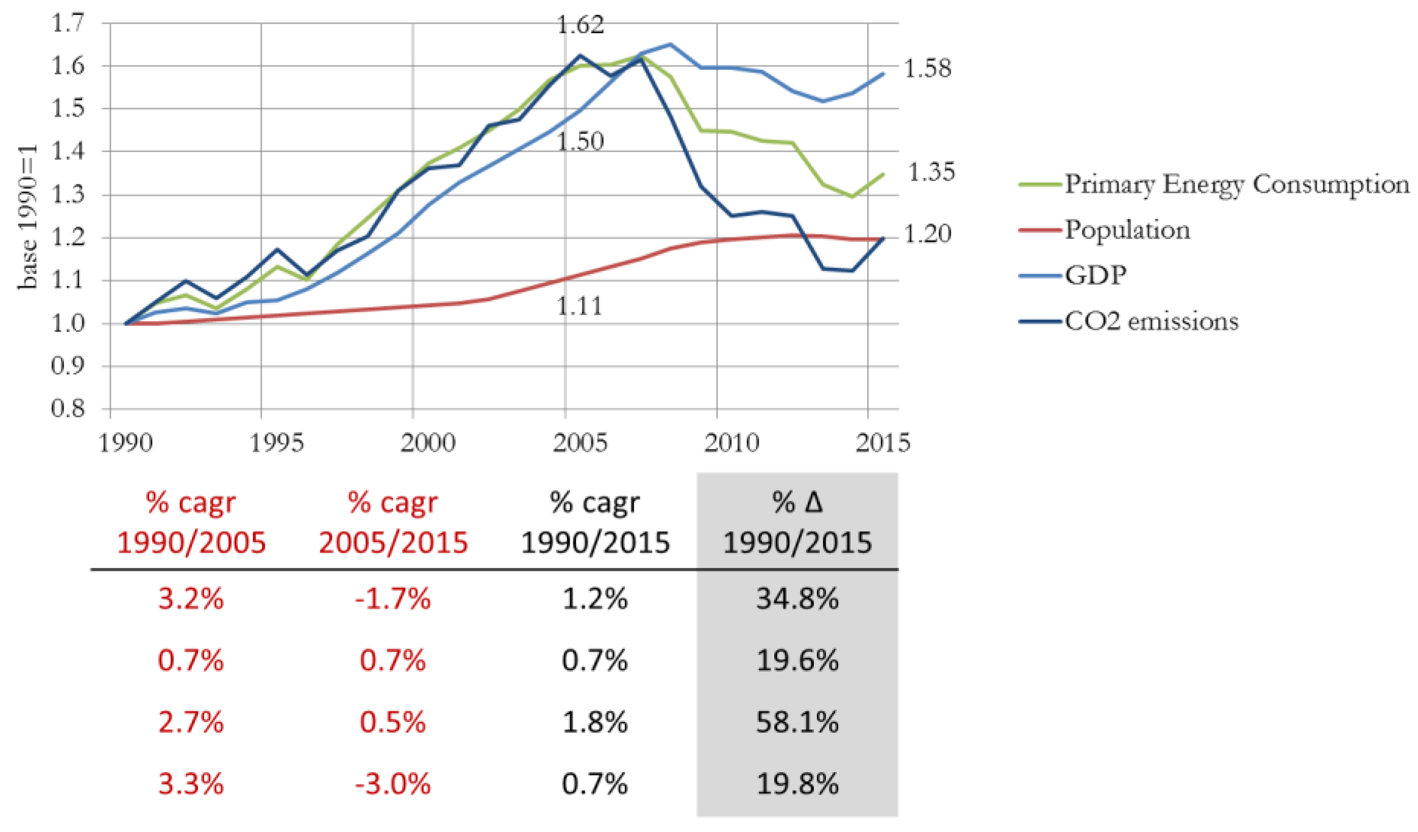
3.1. Evolution of Main Carbon-Related Magnitudes

Human and economic activity is related to energy consumption and carbon dioxide emissions. In Figure 4, we see the evolution of four key parameters for the period 1990–2015: population, gross domestic product (GDP), primary energy demand, and CO₂ emissions. When energy comes from different sources (not just electricity) it is usually expressed in tons of oil equivalent (toe; 1 toe = 11.63 MWh).

Taking values in 1990 as the baseline, the evolution of the four previous magnitudes can be compared in Figure 5 Between 1990 and 2005, a high rate of economic growth (GDP) can be seen: 2.7% in Spain vs. 3.1% in the European Union (EU). By contrast, in the period 2005–2015, the years of crisis and subsequent recovery can clearly be observed, with a GDP increase of 0.5% in Spain vs. 1% in EU). The impact on primary energy consumption was 3.2% and −1.7% in each period. All these percentage values correspond to the compound annual growth rate (CAGR).

During these 25 years, the population in Europe grew at 0.3% (CAGR), whereas Spain presented a strong growth of 0.7%. While the population of Europe grew 7% in this period in accumulated terms, Spain reached an almost 20% increase, a value consistent with other not fully-developed countries and, therefore, with greater energy requirements.

These values can be expressed in terms of the Kaya identity factors (Equation (1)), as seen in

Table 3. Factors of the Kaya identity for Spain (baseline: 1990).

Factor	Symbol	1990	1995	2000	2005	2010	2015
Population	$P$	1.00	1.02	1.04	1.11	1.20	1.20
GDP per person	$G_p$	1.00	1.03	1.23	1.34	1.33	1.32
Energy Intensity	$I_e$	1.00	1.08	1.07	1.07	0.91	0.85
Carbon footprint of energy	$F_e$	1.00	1.00	0.99	1.01	0.87	0.89
CO2 emissions	$C$	1.00	1.17	1.36	1.62	1.25	1.20

.

The emissions produced between 1990 and 2015 grew by 20%, mainly due to the growth of the population by the same proportion, 20%, in addition to an increase of the GDP per person of 32%, which was compensated with improvements in the energy intensity by 15% and in the carbon intensity by 11%.

The process of tertiarization describes the phenomenon of evolving from an economy centered on agriculture, livestock, and fisheries to an economy in which the services sector has the greatest role. Every society begins first with a process of urbanization and industrialization, which is followed by the development of tourism and public services, as well as the incorporation of women into the labor market. This presence of the service sector in the economy translates into jobs, reaching 76% of the active population in Spain.

The relative weight of this sector in GDP, measured through gross value added (GVA) at basic prices, also reached a similar proportion, as depicted in Figure 6. By 2015, at 2015’s prices, the industrial sector represented 33.2% of the GVA, compared to 64.6% for the services sector and 2.2% for agriculture.

The energy consumed by sector is depicted in Figure 7. In this graph, only the energy demand directly related to the economy has been included, that is, the activity sectors 1 to 20, as they are identified in Table 1.

Relating the energy consumed by sector, shown in Figure 7, to its economic contribution, shown in Figure 6, shows that the tertiary sector is less intensive in energy consumption (measured in Mtoe per billion of euro in 2015): 13.9 for services vs. 51.1 for the industry sector and 92.0 for the agricultural and forestry sector.

3.2. Energy Demand Decomposition

We next applied the Laspeyres and LDMI factorial decomposition methods (summarized in Table 2) to the data depicted in Figure 5 (energy) and Figure 6 (activity). The results are shown in Figure 8.

It can be seen that both methods offered quite similar results. As the Laspeyres decomposition is easier to understand, it has been used in the rest of the paper. A more detailed analysis of the results obtained employing the Laspeyres method is depicted in Figure 9.

A decomposition of the energy demand showed the drivers behind the initial variation observed. The variation in energy demand (from 25.3 Mtoes in 1990 to 31.2 in 2015) was explained by an increase (11.7 Mtoes) in the economic activity (A), partially compensated (−2.5 Mtoes) by the structural change from industrial to tertiary economy (S), and a decreasing (−2.4 Mtoes) in intensity or energy efficiency (I).

Following techno-economic factors, it was possible to make an analysis of the past variation in Spain. Following the Annex XIV, part 1 of the Energy Efficiency Directive [58]: “In sectors where energy consumption remains stable or is growing, Member States shall analyze the reasons for it and attach their appraisal to the estimates”.

The activity effect is the measure of value added variation, very much linked to the economic setting. Since 1990, it has been the main effect that explains the variation, shown in Figure 9, of final energy growth. The economic activity trend was linked to the energy demand with a positive elasticity until the appearance of the recession period. Structural changes represent internal evolution with different energy intensities; the evolution of individual branches represents different global energy needs, and they did not grow at the same rate. The energy efficiency depended on technological improvements, fuel substitution, and highest output per unit.

Let us now consider the Laspeyres multiplicative decomposition of energy demand, as depicted in Figure 8. A demand growth of 23% over 1990 was justified by a 50% growth in gross value added (GVA), a −10% reduction due to a structural change in economy (variations of weights between industry, services, and agriculture), and a −10% improvement in energy efficiency or energy use per economic unit.

Around the year 2005, with the economic crisis, an inflection point was seen that invited a more detailed analysis considering two periods: pre-crisis (1990–2005) and post-crisis (2005–2015). Figure 10 shows the results of that analysis, where a pre-crisis growth of energy demand can be seen, mainly based on the positive economic evolution of the country, followed by a post-crisis energy demand decrease, based primarily on a higher energy efficiency (intensity), and secondarily on the tertiarization of the economy (change of economy structure).

Figure 10 shows a different decomposition in both periods. In the second one, due to the crisis, there was a lower demand for energy in all branches of activity, but the contribution of the construction sector was particularly negative. After the crisis, Spain significantly reduced its energy requirements with an improvement of energy efficiency, reinforced by variation in structure branches with different energy intensity compositions, also reducing energy needs.

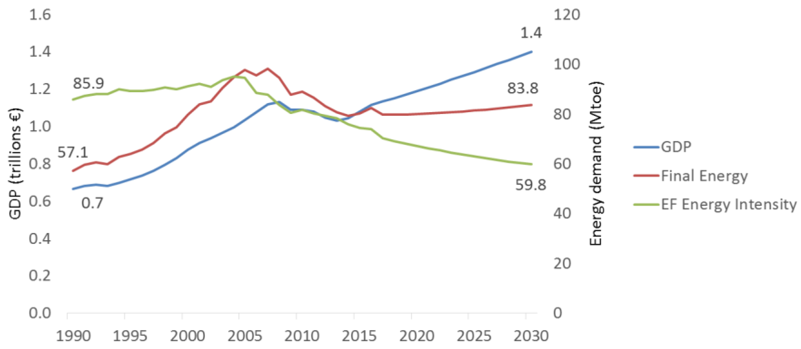
3.3. Population and Aggregated GDP Forecasting

Projections of the United Nations [59,60] estimate for Spain in the year 2030 a low scenario of 44.80 million inhabitants (−0.24%) against a high scenario of 47.37 million inhabitants (+0.18%), as depicted in Figure 11, similar predictions to those of the Spanish National Institute of Statistics [61], which forecast 45.89 million inhabitants, and which could be taken as a central and flat value used to compute the evolution of future energy demand.

Along with population forecasts, to make a projection of long-term energy demand, it is also essential to analyze the growth of the economy. As shown in Table 3, these two magnitudes (population and economy) have been the determining factors in the growth of CO₂ emissions in Spain, having to be compensated with the improvement of energy and carbon intensity.

Regarding GDP growth, projections by the European Commission to 2030 [62] and the OECD [63] forecast the GDP growth of Spain at a 1.9% compound annual growth rate (CAGR). On the other hand, similar results (depicted in Figure 12) were obtained using the previously described time-series models.

Table 4. Growth of GDP for Spain as predicted for several time-series methods.

Time Series Predictor	% CAGR 1990/2005	% CAGR 2005/2015	% CAGR 1990/2015	% CAGR 2015/2030	% Δ 1990/2015	% Δ 2015/2030
Linear regression	2.7%	0.5%	1.8%	2.0%	58.1%	34.9%
Exponential smoothing	2.7%	0.5%	1.8%	0.2%	58.1%	2.9%
Holt-Winters	2.7%	0.5%	1.8%	1.1%	58.1%	17.9%

summarizes the total growth (% Δ) and the CAGR predicted using three time-series forecasting methods. The 2% GDP growth (CAGR) obtained using a linear regression time-series predictor was the same as the forecast published in a recent report driven by the Spanish Government [1]. This value is also very similar to the 1.9% EU and OECD predictions. For these reasons, linear regression was employed to make time-series predictions in the following sections of the paper.

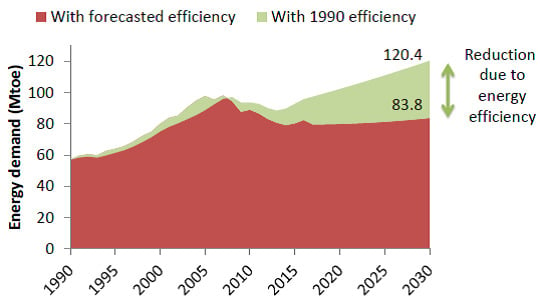
3.4. Energy Demand Forecasting

To forecast the energy demand, the procedure described in Figure 3 was followed. The final energy demand was disaggregated into the $n=30$ level-1 components described in Figure 2 and Table 1. Later, for the sake of representation, sectors 1 to 20 have been grouped into level-2 components (agriculture and forestry, industry and services).

The results are shown in Figure 13, where it can be seen that the energy demand of the activities related to transport represented the largest share of 2015 (42%), while the energy supplied to Industry, Services, and Agriculture represented 39%, and residential activities accounted for 18%.

For factor decomposition, the Laspeyres method (Equations (9) and (11)) was employed because, as was shown earlier, it offered very similar results to LMDI and it is easier to understand. Thus, each of the $n=30$ activity sectors was decomposed into $f=3$ factors, obtaining a total of $m=n·f=30·3=90$ time-series.

To obtain the 2030 horizon forecast for any of the $m=90$ disaggregated time series, a linear regression method was then employed, because, as shown previously, it offered the most accurate predictions in population and GDP forecasts.

The results for the five most energy-demanding level-2 components (as described in Figure 2) are summarized in Figure 14.

Finally, in the third and last step of the proposed methodology (Figure 3), the $m=90$ forecasted values were aggregated to obtain a prediction of the final energy demand. The results are depicted in Figure 15, where the level-2 components are also shown.

4. Discussion

In Figure 16, the final energy demand (red line) and GDP (blue line) are compared. They show a coupled evolution in the pre-crisis period (1990–2005). However, in the post-crisis scenario (2005–2030), they behave in an uncoupled way due to increasing energy efficiency, depicted in the graph by decreasing energy intensity (green line).

The energy intensity had a value of 85.9 toe/M€ in 1990, it was slightly flat till 2005, and decreased to a value of 74.4 in 2015. In Spain, energy efficiency is driven by the European Directive on Energy Efficiency [58] and its transposition into the Spanish legal system. Energy intensity was reduced in Spain by 18.4% between 2000 and 2015, mainly in the post-crisis period, reaching recent reductions of −0.6% in 2016 and −5.0% in 2017. Projecting this trend, the energy intensity will reach a value of 59.8 toe/M€ in 2030.

Some other works have also addressed long-term energy demand prediction for Spain. The results of the present paper were compatible with the findings in Reference [38], which used a similar methodological approach. However, our approach had three main improvements: (a) it employed data spans to 2015 (instead of 2012), gaining a more precise overlook of the post-crisis period; (b) predictions involved the whole energy demand (and not only electricity), obtaining a more comprehensive view; and (c) through the Kaya identity, it was easier to obtain CO₂ emissions, as they depend on the total energy demand.

The results presented in Reference [39], using an econometric model similar to our approach, were also compatible with our findings, confirming the post-crisis decoupling of economy and energy demand due to improvements in energy efficiency. However, our research presented three advantages: (a) it used a more detailed and precise disaggregation; (b) predictions involved the whole energy demand (and not only electricity); and (c) CO₂ emissions were more easily derived.

Energy is essential for the normal functioning of modern societies, although excessive energy consumption becomes a major problem. The energy resources of the planet have to be consumed in a rational way. Energy industry planners and policy makers need accurate tools for prediction.

The world needs energy to keep developing, with more people accessing better life conditions. Energy demand is closely related to the prosperity of people and the competitiveness of economies, which can be measured by the Human Development Index (HDI) [64]. Their relationship is plotted in Figure 17.

5. Conclusions

The forecasting of energy demand is a key issue for making decisions on future investment needs, and also for monitoring energy policy objectives, both for the reduction of CO₂ emissions and the improvement of energy efficiency. Knowledge of the evolution of demand is also the appropriate way to establish alternative plans to correct our course towards our goals and to carry out permanent monitoring.

Our methodological contribution offers a complement to both traditional and data-driven prediction techniques. The possibility of making an individualized projection for each explanatory key parameter separately improves the observability of each effect and trend in a method of “energy forecast by factorial decomposition.” To the extent that each effect maintains its own trends of activity, efficiency, and structural changes separately, different forecasting techniques have been applied and more accurate predictions have been obtained.

The results found in this paper forecast an energy demand in Spain of 82 millions of tons of oil equivalent for the year 2030. Due to improvements in energy efficiency in the post-crisis period, a decoupling of economy and energy demand has been obtained, with a 30% decrease in energy intensity for the period 2005–2030.

In the coming years, energy demand will continue to grow due to the increasing population and economic development. World future scenarios show a significant increase in energy demand due to the human development of less developed economies. For Spain, our research concluded that energy demand will remain stable in the next decade, despite the foreseen 2% annual growth of its economy. The factorial decomposition methodology used through the paper showed that it is possible to decouple economic growth and energy demand via improved energy efficiency.

Finally, from the energy offer perspective, in the future it will not be affordable to supply energy demand using fossil fuels. Despite their enormous energy concentration and density, they represent the waste of a stored energy reservoir to supply the needs of a few moments in humankind history. The consolidation of renewable energies and increasing energy efficiency will reduce future need of fossil fuels.

References

1. World Energy Council. World Energy Trilemma Index 2018; World Energy Council: London, UK, 2018; Available online: https://www.worldenergy.org/publications/2018/trilemma-report-2018/ (accessed on 2 May 2019).
2. European Commission. Energy Roadmap 2050; European Commission: Luxembourg, European Union, 2011; Available online: https://ec.europa.eu/energy/sites/ener/files/documents/2012_energy_roadmap_2050_en_0.pdf (accessed on 2 May 2019).
3. World Energy Council. World Energy Scenarios 2016; World Energy Council: London, UK, 2016; Available online: https://www.worldenergy.org/publications/2016/world-energy-scenarios-2016-the-grand-transition/ (accessed on 2 May 2019).
4. Hong, T.; Pinson, P.; Fan, S.; Zareipour, H.; Troccoli, A.; Hyndman, R.J. Probabilistic energy forecasting: Global energy forecasting competition 2014 and beyond. Int. J. 2016, 32, 896–913. [Google Scholar] [CrossRef]
5. Ciulla, G.; Brano, V.L.; D’Amico, A. Modelling relationship among energy demand, climate and office building features: A cluster analysis at European level. Appl. Energy 2016, 183, 1021–1034. [Google Scholar] [CrossRef]
6. Liang, Y.; Niu, D.; Cao, Y.; Hong, W.C. Analysis and modeling for China’s electricity demand forecasting using a hybrid method based on multiple regression and extreme learning machine: A view from carbon emission. Energies 2016, 9, 941. [Google Scholar] [CrossRef]
7. Rehman, S.; Cai, Y.; Fazal, R.; Das Walasai, G.; Mirjat, N. An integrated modeling approach for forecasting long-term energy demand in Pakistan. Energies 2017, 10, 1868. [Google Scholar] [CrossRef]
8. Hayes, B.; Gruber, J.; Prodanovic, M. Short-term load forecasting at the local level using smart meter data. In Proceedings of the 2015 IEEE Eindhoven PowerTech, Eindhoven, The Netherlands, 29 June–2 July 2015. [Google Scholar]
9. Nagbe, K.; Cugliari, J.; Jacques, J. Short-term electricity demand forecasting using a functional state space model. Energies 2018, 11, 1120. [Google Scholar] [CrossRef]
10. Ryu, S.; Noh, J.; Kim, H. Deep neural network based demand side short term load forecasting. Energies 2016, 10, 3. [Google Scholar] [CrossRef]
11. Akpinar, M.; Yumusak, N. Year ahead demand forecast of city natural gas using seasonal time series methods. Energies 2016, 9, 727. [Google Scholar] [CrossRef]
12. De Oliveira, E.M.; Oliveira, F.L.C. Forecasting mid-long term electric energy consumption through bagging ARIMA and exponential smoothing methods. Energy 2018, 144, 776–788. [Google Scholar] [CrossRef]
13. Bourdeau, M.; Zhai, X.Q.; Nefzaoui, E.; Guo, X.; Chatellier, P. Modelling and forecasting building energy consumption: A review of data-driven techniques. Sustain. Cities Soc. 2019, 48, 101533. [Google Scholar] [CrossRef]
14. Suganthi, L.; Samuel, A.A. Energy models for demand forecasting—A review. Renew. Sustain. Energy Rev. 2012, 16, 1223–1240. [Google Scholar] [CrossRef]
15. Çevik, H.H.; Çunkaş, M. Short-term load forecasting using fuzzy logic and ANFIS. Neural Comput. Appl. 2015, 26, 1355–1367. [Google Scholar] [CrossRef]
16. Singh, S.; Yassine, A. Big data mining of energy time series for behavioral analytics and energy consumption forecasting. Energies 2018, 11, 452. [Google Scholar] [CrossRef]
17. Chen, Y.; Hong, W.C.; Shen, W.; Huang, N. Electric load forecasting based on a least squares support vector machine with fuzzy time series and global harmony search algorithm. Energies 2016, 9, 70. [Google Scholar] [CrossRef]
18. Bouktif, S.; Fiaz, A.; Ouni, A.; Serhani, M. Optimal deep learning lstm model for electric load forecasting using feature selection and genetic algorithm: Comparison with machine learning approaches. Energies 2018, 11, 1636. [Google Scholar] [CrossRef]
19. Akhwanzada, S.A.; Tahar, R.M. Strategic forecasting of electricity demand using system dynamics approach. Int. J. Environ. Sci. Dev. 2012, 3, 328. [Google Scholar]
20. Roming, N.; Leimbach, M. Econometric Forecasting of Final Energy Demand Using in-Sample and Out-of-Sample Model Selection Criteria; Potsdam Institute for Climate Impact Research: Potsdam, Germany, 2015. [Google Scholar]
21. Halvorsen, R. Econometric Models of U.S Energy Demand; United States Department of Energy Office of Scientific and Technical Information: Washington, WA, USA, 1978.
22. Ghods, L.; Kalantar, M. Different methods of long-term electric load demand forecasting: A comprehensive review. Iran. J. Electr. Electron. Eng. 2011, 7, 249–259. [Google Scholar]
23. Ghalehkhondabi, I.; Ardjmand, E.; Weckman, G.R.; Young, W.A. An overview of energy demand forecasting methods published in 2005–2015. Energy Syst. 2017, 8, 411–447. [Google Scholar] [CrossRef]
24. Lin, J.; Zhu, K.; Liu, Z.; Lieu, J.; Tan, X. Study on A Simple Model to Forecast the Electricity Demand under China’s New Normal Situation. Energies 2019, 12, 2220. [Google Scholar] [CrossRef]
25. Ha, S.; Tae, S.; Kim, R. Energy Demand Forecast Models for Commercial Buildings in South Korea. Energies 2019, 12, 2313. [Google Scholar] [CrossRef]
26. Gómez, M.; Ciarreta, A.; Zarraga, A. Linear and nonlinear causality between energy consumption and economic growth: The case of Mexico 1965–2014. Energies 2018, 11, 784. [Google Scholar] [CrossRef]
27. Hall, L.M.; Buckley, A.R. A review of energy systems models in the UK: Prevalent usage and categorisation. Appl. Energy 2016, 169, 607–628. [Google Scholar] [CrossRef] [Green Version]
28. Inglesi-Lotz, R.; Pouris, A. On the causality and determinants of energy and electricity demand in South Africa: A review. Energy Sources Part B Econ. Plan. Policy 2016, 11, 626–636. [Google Scholar] [CrossRef] [Green Version]
29. Verleger, P.K. An econometric analysis of the relationships between macroeconomic activity and US energy consumption. In Energy Modeling: Art Science Practice; Routledge: London, UK, 2016; pp. 62–102. [Google Scholar]
30. Duscha, V.; Fougeyrollas, A.; Nathani, C.; Pfaff, M.; Ragwitz, M.; Resch, G.; Walz, R. Renewable energy deployment in Europe up to 2030 and the aim of a triple dividend. Energy Policy 2016, 95, 314–323. [Google Scholar] [CrossRef]
31. Kabir, E.; Kumar, P.; Kumar, S.; Adelodun, A.A.; Kim, K.H. Solar energy: Potential and future prospects. Renew. Sustain. Energy Rev. 2018, 82, 894–900. [Google Scholar] [CrossRef]
32. Quintana-Rojo, C.; Callejas-Albiñana, F.E.; Tarancón, M.A.; del Río, P. Identifying the Drivers of Wind Capacity Additions: The Case of Spain. A Multiequational Approach. Energies 2019, 12, 1944. [Google Scholar] [CrossRef]
33. Navamuel, E.L.; Morollón, F.R.; Cuartas, B.M. Energy consumption and urban sprawl: Evidence for the Spanish case. J. Clean. Prod. 2018, 172, 3479–3486. [Google Scholar] [CrossRef]
34. Abdelradi, F.; Serra, T. Asymmetric price volatility transmission between food and energy markets: The case of Spain. Agric. Econ. 2015, 46, 503–513. [Google Scholar] [CrossRef]
35. Gokmenoglu, K.; Kaakeh, M. Causal relationship between nuclear energy consumption and economic growth: case of Spain. Strateg. Plan. Energy Environ. 2018, 37, 58–76. [Google Scholar] [CrossRef]
36. Cansino, J.M.; Sánchez-Braza, A.; Rodríguez-Arévalo, M.L. Driving forces of Spain׳ s CO2 emissions: A LMDI decomposition approach. Renew. Sustain. Energy Rev. 2015, 48, 749–759. [Google Scholar] [CrossRef]
37. Mbarek, M.B.; Boukarraa, B.; Saidi, K. Role of energy consumption and economic growth in the spread of greenhouse emissions: empirical evidence from Spain. Environ. Earth Sci. 2016, 75, 1161. [Google Scholar] [CrossRef]
38. Pérez-García, J.; Moral-Carcedo, J. Analysis and long term forecasting of electricity demand trough a decomposition model: A case study for Spain. Energy 2016, 97, 127–143. [Google Scholar] [CrossRef]
39. García-Gusano, D.; Suárez-Botero, J.; Dufour, J. Long-term modelling and assessment of the energy-economy decoupling in Spain. Energy 2018, 151, 455–466. [Google Scholar] [CrossRef]
40. Eurostat. Available online: https://ec.europa.eu/eurostat (accessed on 2 May 2019).
41. Eurostat. Population (Demography, Migration and Projections). Available online: https://ec.europa.eu/eurostat/web/population-demography-migration-projections/data/main-tables (accessed on 2 May 2019).
42. Eurostat. Structural Business Statistics Global Business Activities. Available online: https://ec.europa.eu/eurostat/web/structural-business-statistics/data/main-tables (accessed on 2 May 2019).
43. Eurostat. Energy. Available online: https://ec.europa.eu/eurostat/web/energy/data/database (accessed on 2 May 2019).
44. Eurostat. Climate Change. Available online: https://ec.europa.eu/eurostat/web/climate-change/data/database (accessed on 2 May 2019).
45. Kaya, Y.; Yokobori, K. Environment, Energy, and Economy: Strategies for Sustainability; United Nations University Press: Tokyo, Japan, 1997. [Google Scholar]
46. Ang, B.W.; Zhang, F.Q. A survey of index decomposition analysis in energy and environmental studies. Energy 2000, 25, 1149–1176. [Google Scholar] [CrossRef]
47. Quan, L. Factors Analysis and Empirical Study on Energy Consumption in China: Based on Laspeyres Index Decomposition. Technol. Econ. 2011, 30, 83–86. [Google Scholar]
48. Sun, W.; Cai, H.; Wang, Y. Refined Laspeyres Decomposition-Based Analysis of Relationship between Economy and Electric Carbon Productivity from the Provincial Perspective—Development Mode and Policy. Energies 2018, 11, 3426. [Google Scholar] [CrossRef]
49. Jenne, J.; Cattell, R. Structural change and energy efficiency in industry. Energy Econ. 1983, 5, 114–123. [Google Scholar] [CrossRef]
50. Ang, B.W.; Zhang, F.Q.; Choi, K.H. Factorizing changes in energy and environmental indicators through decomposition. Energy 1998, 23, 489–495. [Google Scholar] [CrossRef]
51. Ang, B.W.; Liu, F.L. A new energy decomposition method: perfect in decomposition and consistent in aggregation. Energy 2001, 26, 537–548. [Google Scholar] [CrossRef]
52. Ang, B.W.; Liu, F.L.; Chung, H.S. A generalized Fisher index approach to energy decomposition analysis. Energy Econ. 2004, 26, 757–763. [Google Scholar] [CrossRef]
53. Diewert, W.E. Index Numbers; Department of Economics, University of British Columbia: Vancouver, Canada, 2007. [Google Scholar]
54. Xue, B.; Geng, J. Dynamic transverse correction method of middle and long term energy forecasting based on statistic of forecasting errors. In Proceedings of the 2012 10th International Power Energy Conference (IPEC), Ho Chi Minh City, Vietnam, 12–14 December 2012. [Google Scholar]
55. James, G.; Witten, D.; Hastie, T.; Tibshirani, R. An Introduction to Statistical Learning; Springer: New York, NY, USA, 2013; pp. 61–63. [Google Scholar]
56. Montgomery, D.C.; Jennings, C.L.; Kulahci, M. Exponential Smoothing Methods. In Introduction to time Series Analysis and Forecasting; John Wiley & Sons: Hoboken, NJ, USA, 2015. [Google Scholar]
57. Gelper, S.; Fried, R.; Croux, C. Robust forecasting with exponential and Holt–Winters smoothing. J. Forecast. 2010, 29, 285–300. [Google Scholar]
58. Directive 2012/27/EU of the European Parliament and of the Council of 25 October 2012 on energy efficiency. Available online: https://eur-lex.europa.eu/eli/dir/2012/27/oj (accessed on 2 May 2019).
59. United Nations Population Division. The 2015 Revision of the UN’s World Population Projections. Popul. Dev. Rev. 2015, 41, 557–561. [Google Scholar] [CrossRef]
60. Key Findings and Advance Tables. In World Population Prospects; The 2015 Revision; United Nations Population Division: New York, NY, USA, 2015.
61. INE. Proyecciones de Población 2016–2066. 2016. Available online: https://www.ine.es/prensa/np994.pdf (accessed on 2 May 2019).
62. Capros, P.; De Vita, A.; Tasios, N.; Siskos, P.; Kannavou, M.; Petropoulos, A.; Paroussos, L. EU Reference Scenario 2016-Energy, Transport and GHG Emissions Trends to 2050; European Commission Directorate: Luxembourg, European Union, 2016; Available online: https://doi.org/10.2833/9127 (accessed on 2 May 2019).
63. OECD. GDP Long-Term Forecast (Indicator). 2018. Available online: https://doi.org/10.1787/d927bc18-en (accessed on 2 May 2019).
64. Sanz-Oliva, J. (Coord.) Análisis Y Propuestas Para La Descarbonización. Gobierno de España. Available online: https://drive.google.com/file/d/1ECtDV6Nhg5qzvLj9pwQ5d-Gx7KzuiFFn/view (accessed on 2 May 2019).
Figure 1. Energy trilemma.
Energies 12 03095 g001
Figure 2. Structure of energy demand disaggregation.
Energies 12 03095 g002
Figure 3. Procedure to obtain the energy demand forecast.
Energies 12 03095 g003
Figure 4. Magnitudes (absolute values) of the Kaya identity for Spain (1990–2015): (a) population; (b) gross domestic product; (c) primary energy demand; (d) CO2 emissions.
Energies 12 03095 g004
Figure 5. Magnitudes (base 1990 = 1) of the Kaya identity for Spain (1990–2015).
Energies 12 03095 g005
Figure 6. Gross value added for Spain (1990–2015). Units: billions of euros at 2015 prices.
Energies 12 03095 g006
Figure 7. Energy demand (Mtoes) for Spain (1990–2015): Industry, Services, and Agriculture and Forestry.
Energies 12 03095 g007
Figure 8. Energy demand multiplicative decomposition: (a) activity; (b) structure; (c) energy intensity.
Energies 12 03095 g008
Figure 9. Energy demand Laspeyres decomposition (toes) for Spain (1990–2015).
Energies 12 03095 g009
Figure 10. Energy demand Laspeyres decomposition for Spain during the pre-crisis (1990–2005) and the post-crisis (2005–2015) periods.
Energies 12 03095 g010
Figure 11. Evolution and forecast of population for Spain [60].
Energies 12 03095 g011
Figure 12. Evolution of GDP and its forecast for Spain.
Energies 12 03095 g012
Figure 13. Disaggregation of final energy (Mtoe) for Spain. Inner: 1990; middle: 2015; outer: 2030 (forecast).
Energies 12 03095 g013
Figure 14. Projection of indices (left) and decomposition of energy demand (right) for 2015–2030: (a) industry; (b) services; (c) passenger transport; (d) freight transport; (e) residential.
Energies 12 03095 g014
Figure 15. Final energy demand forecast (Mtoe) for Spain.
Energies 12 03095 g015
Figure 16. Final energy demand (Mtoe), GDP (T€: trillions of €), and energy intensity (toe/M€).
Energies 12 03095 g016
Figure 17. Human Development Index vs. energy consumption (GJ) per capita.
Energies 12 03095 g017