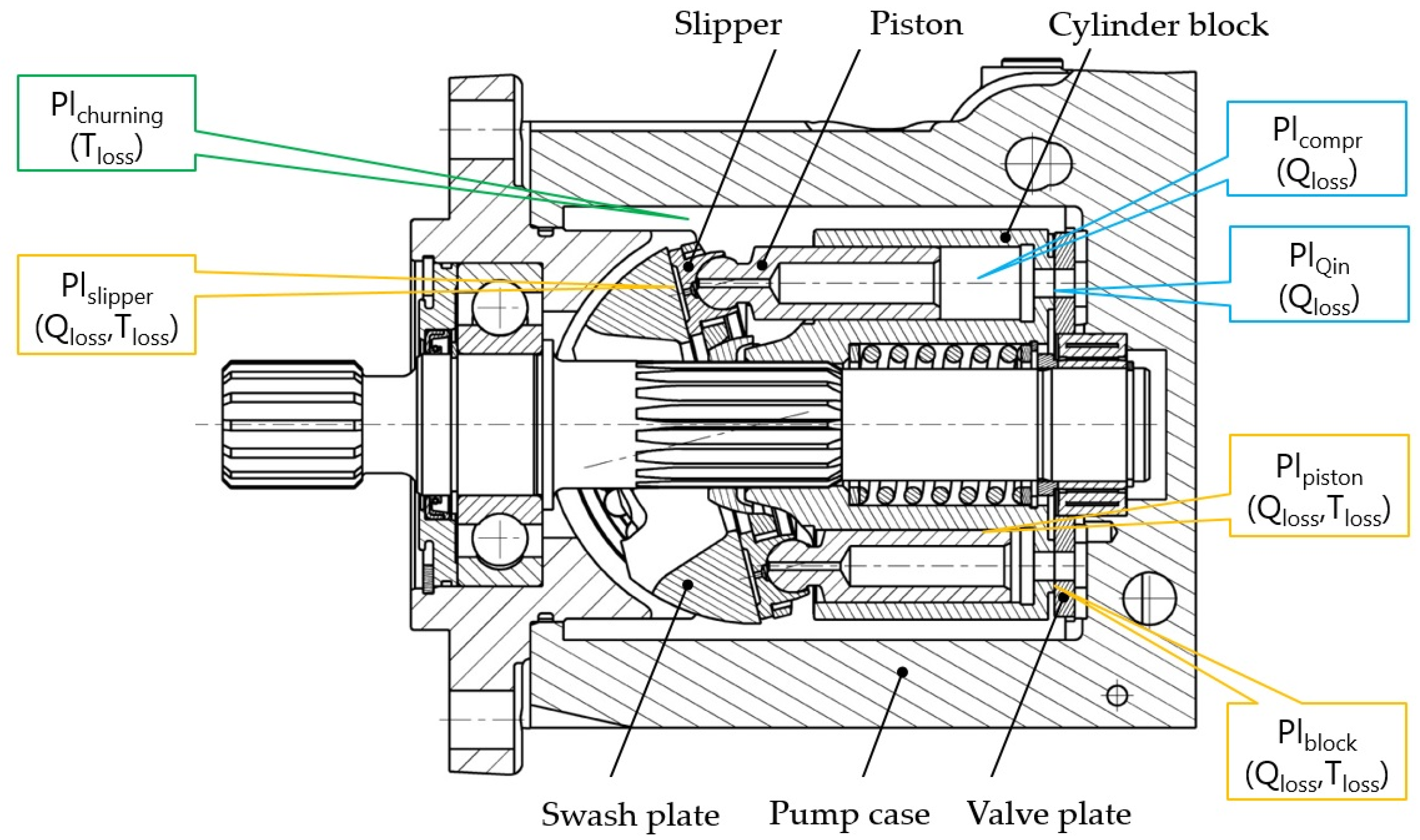
Article

Virtual Assessment and Experimental Validation of Power Loss Contributions in Swash Plate Type Axial Piston Pumps

1
Université de technologie de Compiégne, Roberval Laboratory CNRS FRE 2012, 60203 Compiegne CEDEX, France
2
Maha Fluid Power Research Center, Purdue University, 1500 Kepner Dr., Lafayette, IN 47905, USA
*
Authors to whom correspondence should be addressed.
Energies 2019, 12(16), 3096; https://doi.org/10.3390/en12163096
Submission received: 25 July 2019 / Revised: 5 August 2019 / Accepted: 9 August 2019 / Published: 12 August 2019

Abstract

:
The understanding of the power loss contributions of each loss source is essential for an effective development of swash plate type axial piston pump. However, it is difficult to obtain the assessment of the power loss distribution due to the lack of methodologies that allow an independent evaluation of each source. This paper addresses this challenge using the most recent simulation methods. It describes the determination of each source, along with the corresponding loss of performance, and the principle of their prediction during the design phase. It also reports the validation of the simulation model by comparing the simulated dynamic displacement chamber pressure and the solid body temperature distribution with measurements obtained from a special pump prototype. This proposed virtual assessment of power loss contributions is demonstrated on a commercial hydraulic unit and the detailed results are reported in this paper.

1. Introduction

Swash plate type axial piston pumps (S-APPs) are variable positive displacement machines known for their high-pressure capability, high power density, high-energy efficiency, and great robustness. Thanks to these advantages, S-APPs dominate the high-pressure unit market for agricultural, industrial, and off-highway vehicle applications. Meanwhile, the performance of pumps (and motors) is emphasized in the modern fluid power systems, such as displacement control systems, hydrostatic transmissions, and electro-hydraulic actuation. There is a substantial demand to increase maximum operating pressure, to improve life expectancy, and, above all, to improve energy efficiency.
When developing S-APPs, the top challenge is to design the three lubricating interfaces (piston/cylinder bore interface, cylinder block/valve plate interface, and slipper/swash plate interface). These tribological interfaces must fulfill two functions: sealing the high pressure (up to 50 MPa) fluid in the displacement chambers and bearing the high loads from the chamber pressure. The viscous and mixed friction between the sliding boundaries of these interfaces is the main contribution of the torque loss in S-APPs. Moreover, the gap flow in these interfaces presents itself as the external leakage. Furthermore, the shape of the sealing area of the cylinder block/valve plate lubricating interfaces also determines the port opening timing of the displacement chamber, which further controls the back flow, also known as internal leakage. The experimental determination of the total power loss can lead to a total efficiency, which can be further split into volumetric and hydraulic-mechanical components [1]. This experimental method provides the overall pump characteristics, but not the distribution of the power loss from different sources. Moreover, it can only be performed on a physical prototype. By this approach, the development of S-APPs must involve many iterations of expensive trial-and-error processes. Accurate assessment of the power losses contributions during the design phase is necessary to effectively shorten the development cycle and reduce cost.
Researchers [2,3,4] have tried to evaluate the power loss, friction force, or leakage flow from each individual source experimentally. However, their methods depend on heavily modified and simplified S-APPs, which do not represent a real S-APP in normal operation.
Olsson [5] investigated the power losses of the S-APP in a wide range of operations using the simulation tool CASPAR [6,7]. His investigation involves the simulations of the performance of the slipper/swash plate and the piston/cylinder bore interface. However, the simulation tool used in his study does not consider solid bodies deformations. He took into account experimentally measured churning loss, but the rest of the power loss sources ignored. Zecchi, Mehdizadeh, and Ivantysynova [8] predicted the temperature of the oil in the ports and case of an S-APP base on the simulated power loss from all three lubricating interfaces and from churning effects of the rotating group. The comparison of the predicted and measured results showed a very good agreement. However, the distribution of the losses in the S-APP was not detailed.
Recent developments in the modelling approach for slipper/swash plate interface [9,10,11], piston/cylinder bore interface [12,13,14,15], and cylinder block/valve plate interface [16,17,18] include elastic deformations due to pressure and thermal loads, heat transfer in the solid boundaries, and compressibility of the fluid. Wieczorek and Ivantysynova [7], Seeniraj [19], and Klop [20] developed a lumped parameter model of displacement chamber pressure based on the assumption of uniform pressure in the entire displacement chamber.
Despite significant progress in pump modelling methods, the use of simulation tools is still not a standard part of the S-APP design process. The aim of the paper is to consolidate previous research, to demonstrate the benefits of the above methods, and to describe a novel complete process of determining power loss distribution in S-APP by demonstrating extensive study of commercial pump over a wide range of operations. The simulation tools that were used in this work are all based on the knowledge of the physical phenomena in S-APP with no black box approach nor needs of parameter tuning to match the measurement.
This article describes the fundamental principles of each type of power losses in Section 2. Section 3 illustrates the fluid structure and thermal interaction (FSTI) simulation approach for the three lubricating interfaces and the lump parameter model for the displacement chamber pressure. Section 4 describes the experimental technique of measuring the instantaneous chamber pressure and the temperature distribution in the valve plate used to validate the simulation model in Section 5. The virtual assessment of power loss contributions in the commercial hydraulic unit is discussed in Section 6, followed by the discussion of achieved results in Section 7.

2. Classification of Power Losses

Each S-APP works with viscous and compressible fluid. Therefore, its output hydraulic power is always lower than its input power from the shaft. The difference between the two, which is total power loss of the S-APP, can be primarily divided into volumetric and hydraulic-mechanical losses according to ISO 4391 [1]. These two losses are explained in the following subsections.

2.1. Volumetric Losses

The micron-level lubricating gaps separate the parts in relative motion. The leakage flows occur with the pressure difference across these gaps. The sum of all leakage flows through the lubricating interfaces represent the external leakage of an S-APP. Depending on the pump design, the displacement chamber may periodically create an instantaneous connection between the inlet and the outlet ports resulting in cross-port flow. This back flow from the outlet port to the inlet port forms the internal leakage [21,22]. Furthermore, according to ISO 4391, the compressibility of the fluid results in an additional loss since the outlet flow is reduced in its volume due to higher pressure at outlet port compared to the pressure at inlet suction port. The gap flows, cross-port flows, and fluid compressibility reduce the effective outlet flow. The difference between the effective and the derived theoretical outlet flow defines the total volumetric losses Qloss of an S-APP.

2.2. Hydraulic-Mechanical Losses

Hydraulic-mechanical losses Tloss in a real displacement machine are generated due to friction on moving parts. The torque needed to overcome the viscous friction in lubricating interfaces, as well as solid-state friction or mixed friction if occurring during operation, increases the effective input pump torque. Besides that, hydraulic-mechanical losses also include the torque needed to overcome the friction in roller bearings and sealing components, and the losses caused as a consequence of the rotation of the pump parts in the case filled by fluid, denoted as churning losses. The timing of the pressure raise and drop, and pressure overshooting also able to alter the effective input shaft torque from the theoretical value, which, according to ISO 4391, needs to be accounted as hydraulic-mechanical losses.

2.3. Power Losses

The friction and leakage in lubricating interfaces between piston/cylinder bore, slipper/swash plate, and cylinder block/valve plate are the major sources of the power loss of S-APPs, designated as Plpiston, Plslipper and Plblock respectively. They are shown in Figure 1 together with the power loss due to internal leakage (PlQin), compressibility (Plcompr), and due to churning losses (Plchurning).
All types of power losses depend on operating conditions and their individual assessment is very problematic. Therefore, the standard mapping of power losses over the entire operating range is based on measuring the total pump efficiency by comparing input and output power:
η t = P o u t P i n = Q e · Δ p T e · ω = η v o l · η h m
The total efficiency can then be divided into the volumetric and hydraulic-mechanical losses by knowing the derived displacement volume Vi [21,23]. The ratio of the effective output flow to the derived output flow defines volumetric efficiency of the pump:
η v o l = Q e Q i = Q e n · V i
and volumetric losses Qloss are defined as:
Q l o s s = n · V i Q e
The ratio of the derived input torque and effective input torque defines hydraulic-mechanical efficiency:
η h m = T i T e = Δ p · V i 2 π · T e
and hydraulic-mechanical losses Tloss are defined as:
T l o s s = T e Δ p · V i 2 π
Determination of the derived displacement volume Vi is crucial for calculating volumetric and hydraulic-mechanical losses. The Toet method [23,24] was used for this paper when Vi is defined from measured Δp – Qe characteristic at constant pump speed n by extrapolation of measured flows to Δp equal to zero.

3. Simulation Model

Performance in the lubricating interfaces for a given S-APP strongly depends on the operating conditions defined by combinations of the rotational speed of the shaft, inlet pressure and temperature, outlet pressure and temperature, temperature of the fluid in the pump case and on the pump displacement set by the swash plate angle. The fluid structure and thermal interaction model assumes all these parameters of operating conditions as constant steady state conditions. The model consists of different modules solving elementary physical domains.

3.1. Displacement Chamber Pressure Modul

The simulation of the individual lubricating interfaces is conditional upon the correct determination of the acting forces and moments, which mainly concerns the pressure in the displacement chamber. This module simulates:
  • instantaneous displacement chamber pressure in each displacement chamber;
  • effective input shaft torque;
  • effective outlet flow;
  • volumetric losses due to compressibility and internal leakages.
Assuming the adiabatic bulk modulus Ka, the pressure in the control volume VDCi shown in Figure 2 is controlled by:
d p D C i d t = K a V D C i ( Q r i Q S K i Q S B i Q S G i d V D C i d t )
The last term represents the rate of change of displacement chamber volume; the terms QSKi, QSBi, QSGi represent external leakage flows through interfaces and Qri is the resultant flow of individual displacement chamber calculated as:
Q r i = Q r H P i + Q r L P i
where QrHPi is the flow rate between a single displacement chamber and the high-pressure port with pressure pHP, while QrLPi is the flow rate between the displacement chamber and the low-pressure port with pressure pLP. These flow rates are calculated using the orifice equation:
Q r L P i = c q · A L P i · 2 | p D C i p L P | ρ · s i g n ( p D C i p L P )
According to the sign convention used above, a positive sign corresponds to positive flow entering the displacement chamber while a negative sign to flow exiting the displacement chamber. The empirical value is used for discharge flow coefficient cq and AHPi, ALPi represent the minimal cross section areas through which the fluid flows from the pump ports to the displacement chamber and vice versa. They are functions of the shaft angle ϕ and depend on valve plate geometry.
The displacement chamber pressure is used for calculation of the load conditions of individual parts of the rotating group, providing necessary input data for simulation of performance in lubricating interfaces. Furthermore, the results of effective input shaft torque and outlet flow allow to determine the total power loss in displacement chambers as difference between mechanical input and hydraulic output power:
P l D C = P i n P o u t = T e · ω Q e · ( p H P p L P )
Knowing the displacement chamber pressure allows to determine the compression losses. Since the compression in hydrostatic pumps is fast, the adiabatic bulk modulus is assumed:
The effective outlet fluid volume during one revolution is reduced by a value ΔVB as illustrated in Figure 3 when for a given operating speed n, the effective outlet flow of a pump is reduced by an amount [21]:
Q s k = n · Δ V B
The relationship between the changing pressure and changing volume in compression and expansion phases can be expressed using the instantaneous adiabatic bulk modulus Ka:
d p = K a V d V
The energy required for compression of a specific amount of fluid from pressure p1 to p2, while its volume is decreasing from VB to VC, is defined as follows:
E c = V B V C p d V
On the other side, part of compression energy can be recovered during expansion of the fluid from the volume VD to VA:
E e = V D V A p d V
Power losses due to the compressibility in an S-APP can be defined as the difference between the input shaft power and the output hydraulic power when considering no cross porting, no friction, and no external leakage, which yields:
P l c o m p r = ( E c E e ) Δ t = ( E c E e ) · n 60
Power losses due to internal leakage are then:
P l Q i n = P l D C P l c o m p P l Q e x
where the total power losses due external leakage PlQex are determined by FSTI model explained below.

3.2. Lubricating Interface FSTI Model

FSTI model predicts the performance in three main lubricating interfaces at steady state operation assuming a full fluid film lubrication. The individual parts of the rotating group are under the large external loads and their relative motions are possible only due to the fluid layers between them, which must provide a sufficient lubrication. The pressure field generated in these fluid layers must support the external loads acting on the parts and prevent the asperity contact that can lead to the wear and potential failure of a pump.
The total amount of power loss in these lubricating interfaces is associated with the leakage flows due to the pressure difference across the gaps and with the energy dissipation due to the viscous friction in the fluid layers. Along with the fluid viscosity, the thickness of the fluid layer directly affects the generation of the total energy dissipation in the lubricating interface, which is transformed into the heat. The gap height is not uniform over the sealing land due to design dimensions and due to the contribution of pressure and thermal deformations of solid bodies. All three interfaces are subjected to the same physical phenomena and are modeled using the same principle structure as shown in Figure 4. Elementary domains are solved in different sub-modules coupled by data interpolation.
The non-isothermal fluid flow sub-module governed by the Reynolds and convective-diffusive energy equation, solves the pressure and thermal field in the fluid film, and the heat flux qS from the gap to solid bodies.
The Reynolds equation determines the pressure field distribution in the gaps as shown in Equation (16) using the distributed viscosity and density within the gaps with the deformation, the inclination, and the macro and micro motion of the solid parts. The relative position between the parts is simulated by integration of micro motion that is calculated using Newton’s method to satisfy force balance between fluid forces in the interfaces and the external load on the solid bodies [7].
i Γ i ( p ) i A i = V S d V
The fluid and structure interaction is solved in an iterative loop as shown in Figure 4, when the pressure deformations Δh of the solid bodies are considered in the gap height [9,11,13,16].
The energy equation solves the temperature distribution in the fluid domain, considering convection, as shown as the first term on the left side in Equation (17), diffusion, the second term on the left side, and heat generation due to viscous dissipation, as the right side in Equation (17) [7,15]:
ρ c p V · θ · ( λ θ ) = μ D
The mechanical dissipation function ØD represents the source term in the energy equation. It determines the heat generated by the viscous shear of the fluid, and in the Cartesian coordinate system is expressed as [7]:
D = ( u ^ z ^ ) 2 + ( v ^ z ^ ) 2
where the terms u ^ and v ^ define the fluid velocities distribution in circumferential and axial direction of the gap.
The distribution of body temperature θb is calculated using FEM solver with the heat flux qS as the boundary condition. The temperature distribution on the running surface θS then becomes the thermal boundary condition for the fluid temperature in FVM model. Furthermore, the distribution of body temperature θb is used as the thermal load to calculate the solid body thermal deflection that is also considered in the gap height. This fluid structure and thermal interactive problem is solved in an outer iterative loop as shown in Figure 4, which allows the fluid film thickness to be determined [11,13,18].
The integration of the dissipation function throughout the volume of the fluid film determines the total energy dissipation in the lubricating interfaces [18]:
P l = V μ D d V
The leakage flow and pressure difference across the gap determines the volumetric component of total energy dissipation Pl:
P l V o l = Q e x · Δ p
when leakage flow Qex depends on the fluid velocity v ^ , the length b and the height h of the gap:
Q e x = b 0 h v ^ d h
Hydraulic-mechanical losses are then determined as:
P l H M = P l P l V o l
Particularly important input parameters are the properties of the hydraulic fluid with which the pump operates. The density and bulk modulus of the hydraulic fluid have a major influence on the pressure in the displacement chamber and consequently on loads of the individual parts. Further, the viscosity of the fluid greatly affects the overall power losses in the lubricating interfaces. The fluid properties vary widely with instantaneous pressure and temperature. Thanks to the measurement provided by a specialize laboratory, it was possible to create the mathematical model that determined the correct properties of the fluid at any machine operation and at any point in the lubricating interface with the appropriate pressure and temperature. The hydraulic oil used was an ISO 46 viscosity grade. Its density and viscosity were measured in the range of pressure up to 1200 bar and in the range of temperature up to 120 °C. The density dependence on pressure and temperature is expressed by following empirical equation with reference pressure pref as 1 bar and reference temperature θre f as 25 °C:
ρ ( p , θ ) = ρ 0 [ 1 + c 1 ( θ θ r e f ) + c 2 ( p p r e f ) + c 3 ( p p r e f ) 2 + + c 4 ( θ θ r e f ) ( p p r e f ) + c 5 ( θ θ r e f ) ( p p r e f ) 2 ]
where c1, c2, c3, c4 and c5 are empirical coefficients.
The definition of the bulk modulus is:
K ( p , θ ) = ρ ( p , θ ) ( ρ p ) θ
An empirically derived exponential model published by Roelands [25] was applied for the relationship of the oil viscosity with the temperature and pressure:
μ ( p , θ ) = 10 ^ ( G 0 ( 1 + p 2000 ) C 2 · log ( 1 + θ 135 ) + D 2 ( 1 + θ 135 ) S 0 1.2 )
where G0, C2, D2, and S0 are empirically derived coefficients.
Figure 5 shows a high correlation of the empirical models of density and viscosity with the measured values, more specifically, absolute average deviation (ADD) is 0.01% for density and 1.2% for viscosity.
Within the simulated performance from this previously mentioned model, this proposed virtual assessment study focuses on:
  • Volumetric losses due to external leakages;
  • Viscous friction forces in the lubricating gaps;
  • Lubricating fluid film thickness, pressure and thermal fields;
  • Viscous energy dissipated in each of the three interfaces;
  • Pressure and thermal deformation and temperature distribution of the bounding solid bodies;
  • The indication of lubricating fluid film collapse.

4. Experimental Approach

Prior to using the above-mentioned simulation tool for virtual assessment of the power loss contributions in S-APP, its experimental validation was performed on a commercial hydraulic unit specified in Table 1.
The ideal validation process should include measuring specific parameters of all power loss sources. However, this kind of experiments require the introduction of many measuring tools with large modifications of the reference machine. The main objective is to analyze the performance of a real machine; therefore, the selection of experiments focused on achieving the maximum amount of data without modifying the pump that could affect its behavior. In order to validate the pressure model, the reference pump was equipped with a piezoelectric pressure sensor for measurement of displacement chamber pressure. Furthermore, the numerically calculated temperature distribution in the valve plate body is compared against the measurements from thirty thermocouples installed in the valve plate under the running surface.

4.1. Dispalcement Chamber Pressure Measurement

The bore, drilled from the outer cylinder block housing and closed by the conical expander, provides a connection between the pressure sensor and the displacement chamber as shown in Figure 6. The created volume between the sensor and displacement chamber increases the dead volume of the displacement chamber, but is very small, and its impact on the behavior of displacement chamber pressure is negligible. The possible influence of the Helmholtz resonance on the measurement was avoided by designing the dimensions for the pressure sensor cavity in relation to the natural pump frequency at maximum speed. Unfortunately, the hole for introducing of the pressure sensor reduced the walls of the material between the cylinder bores. The FEA analysis revealed that the deformation of the block bores adjacent to the drilling for the sensor had changed approximately by 50% in comparison to the original design. This increased deformation, which is proportional to the operating pressure, significantly changes the effective clearances between piston and cylinder bore during high-pressure operation. Therefore, the maximum working pressure of the modified pump was limited to 170 bar to ensure the normal and safe operation during the test. The wireless telemetry system transmitted the amplified signal from pressure sensor as shown in Figure 7. The cable, guided in the shaft, ensured the connection between the sensor and the telemetry system. The telemetry system mounted on the rear of the pump had no effect on the pump operation. The optical sensor measured the angular position of the shaft and thus allowed the synchronization of the pressure sensor signal with the angular position of measured displacement chamber.

4.2. Valve Plate Temperature Distribution Measurement

A set of thirty thermocouples placed 1 mm underneath of the sealing surface of the valve plate measured the solid body temperature distribution as shown in Figure 8. The temperature distribution in valve plate is controlled by the heat flux on its surfaces, most importantly, the sealing surface. The energy dissipation in the fluid film determines the heat flux on the valve plate-sealing surface, which is subsequently transformed into heat energy and into the thermal field of the valve plate respectively. The energy dissipation in the fluid film is highly dependent on the fluid film thickness; therefore, the temperature of the valve plate is an indicator of the thickness of the fluid film. Figure 9 shows the subassembly of the valve plate in the housing of modified pump with the thermocouples, which have a way out from the pump as depicted in Figure 7.

4.3. Operating Conditions and Equipments

The investigation of the pump was performed in various operating conditions. The measurements were taken under steady-state and covered all parameters defined by the ISO 4409 [26] together with displacement chamber pressure, shaft angular position, and temperature from thermocouples as listed in Table 2. All the readings were recorded only when the indicated values of all controlled parameters were within the limits defined by standard with accuracy class B.
The measured speed, pressures, and temperatures at the high-pressure port, the low-pressure port, and the leakage port, were used as accurate input parameters for the simulation model. Other parameters were used for comparison with the simulations results to verify the simulation model.
The gerotor charge pump was removed from the 52 cc unit since its contribution to the power losses are not investigated in this study. An external flow source compensated the volumetric losses in the hydraulic circuit as depicted in Figure 10. The control system required no flow, since the displacement of the pump was set by a fixation of the swash plate in its position using a set screw. The pump was investigated in various combinations of inlet port temperature, displacement, speed and pressure at outlet port listed in Table 3, while the inlet port pressure setting remained at 20 bar.
The steady state test rig consists of two closed-loop circuits. The pump equipped with a pressure transducer and thermocouples was placed in the inner circuit, while the outer circuit controlled the speed and load of the reference pump using variable hydraulic units. For each operating condition, it was necessary to regulate the inlet port temperature so that it remained constant to stabilize all other measured parameters over the time. The variable orifice implemented into the system regulated the amount of flow through the cooler into the tank, and so helped to regulate the inlet pump temperature using the oil from the tank supplied by an external charge pump.

5. Results

Based on the comparison of measured and simulated values of specific parameters, the accuracy of simulation method and thus the accuracy of pump performance prediction is determined. The experimental approach focuses on measuring the displacement chamber pressure and the valve plate temperature. Unfortunately, measurements of other power loss sources were not performed because the priority was to avoid significant modifications of the reference unit. Therefore, the direct comparison of the modeling of other power loss sources is not possible. However, the comparison of the total measured pump losses with the sum of all simulated power losses is an additional, although indirect, validation method with reasonable value.

5.1. Displacement Chamber Pressure

Simulation of displacement chamber pressure, which starts at the outer dead center of the piston (when the piston is in its maximum outer position); depends on precise definition of cross-section areas of the valve plate geometry and on the correct definition of the oil properties. The position sensor recorded the shaft angular position and allowed to align the measured behavior of displacement chamber pressure with the simulation results.
Figure 11 demonstrates the correlation between measured and simulated instantaneous pressure in displacement chamber during transient phases around 180 and 360 degrees. The model is able to predict the pressure behavior during compression and expansion since it captures the slopes as well as starting and ending positions of raising and falling pressure.
The oscillation of the pressure during discharge phases is due to the oscillation of the system pressures in high-pressure line. The simulation model is able to follow this trend in both phase and magnitude, although with small differences that is possible to explain by pressure sensor accuracy. The simulation model showed the similar results in all test conditions.
The simulation model of displacement chamber pressure matches well with measurements over the entire operation range; thus confirm the correct determination of the external loads acting on the parts during simulation of performance in lubricating interfaces, and confirmed the correct prediction of the power losses due to compressibility.

5.2. Valve Plate Temperature

The set of thirty thermocouples positioned over the sealing surface measured the temperature of the valve plate under the surface in contact with the fluid film between the valve plate and the cylinder block. Unfortunately, the three thermocouples were broken during the assembly of the pump prototype due to space limitation problem. That was detected later during testing when they could not be replaced. Finally, only twenty-seven thermocouples were functioning, but still providing enough data to compare with the simulation model. Figure 12 shows an example of the simulated and measured data for defined operating condition. The broken thermocouples are designated as ‘’X’’ in Figure 12 and in Figure 13.
The differences between simulated and measured values of temperature in defined points are shown for better comparison. At high-power operations represented by operating condition in Figure 13a, some points match well with measurements, but the differences in some points were higher, up to 11 °C. At low-power operations represented by operating conditions in Figure 13b the maximum difference was much lower, below 3 °C in all measured points. The average values of absolute errors for the 27 working thermocouples are shown in the Table 4 as an overview of all operations in which the pump was investigated.
The average error in the prediction of the valve plate temperature under the sealing land over a wide range of operating condition is lower than 6 °C. The energy dissipation in the fluid film, which is in the order of few microns, is the results of multi physical phenomena and depends on many input parameters. Therefore, this error is acceptable and the prediction of performance in the lubricating interface between the cylinder block and the valve plate can be considered sufficiently convincing.

5.3. Flow Losses

As previously mentioned, the total volumetric losses of an S-APP depend on the external leakage through the sealing gaps, the internal leakage due to the port opening timing, and the compressibility of the fluid. This section compares the simulated external leakage from all three lubricating interfaces, and the simulated outlet flow with the measured values. To ensure the comparability, the simulations and the measurements were performed under the same operating conditions. Figure 14 shows an example of total leakage flows through individual lubricating interfaces for defined operating conditions as a function of pressure.
Their sum represents the estimated total external leakage of the pump used to compare with the measured drain flow Qc in Figure 15.
The predictions of the external leakage and the effective outlet flow (Figure 16) closely follow the trends of the experimental values. The differences depend on the operating conditions but are always very small compared to the accuracy of the measuring instruments. Is also important to note that tolerances of swash plate fixation system may cause deviation +/–0.2° of swash plate inclination, which corresponds to the outlet flow variations e.g., +/–1 liter per minute at full displacement and at maximum speed.

5.4. Torque Losses

To estimate the churning losses, the pump was set to neutral position and the input torque was measured for different speeds. Then the process was repeated with empty case of the pump. To avoid any issues by the oil absence in the case, the measurements were performed in a short time interval using the ramp control signal for the speed. Therefore, the complete stabilization of all parameters was not possible. However, using the same measurement conditions, the differences of input torque between the oil-filled and the empty case determine the churning losses. Figure 17 shows the churning losses only as a function of the pump speed since they have very similar values for different inlet temperatures.
Figure 18 shows the comparison between the simulated and measured hydraulic-mechanical losses. The simulated losses represent the sum of all hydraulic-mechanical losses determined by FSTI model increased by the appropriate values of measured churning losses. The actual hydraulic-mechanical losses of the pump were determined according to the ISO 4391 using the derived displacement volume Vi.
The predicted hydraulic-mechanical losses are significantly lower than the measured values in all operating conditions. Since the FSTI simulation model assumes the full fluid film lubrication, only the viscous energy dissipation is included in the results. If, due to the design of lubricating interfaces, the fluid film collapses in its thickness, then the pressure field generated in the gap is not able to support the external loads acting on the parts, and the simulation model inserts the numerical force value to achieve a force balance. In this case, mixed or dry friction will be present during a real pump operation. Figure 19 shows the unbalanced forces for each interface in different operating conditions that the software automatically compensates. These unbalanced forces are not included in the simulation results of power losses; however, they indicate the fluid film collapse resulting in mechanical contact between the parts. The unknown coefficients of actual contact friction do not allow the conversion of these unbalanced forces into power losses. However, their presence warns the designer to higher losses and a potential risk of failure. Their elimination must be a priority, although it is not an easy design problem.

6. Distribution of Power Losses within the Pump

The total power losses of the investigated pump were defined according to the process described in Section 2 as a difference between input and output power. Table 5 and Table 6 summarize the distribution of the total power losses within the S-APP of 52 cc size based on a simulation approach over a wide range of operating conditions. The power losses due to the internal leakage and compressibility are determined from the results of displacement chamber pressure module, the churning losses are defined experimentally, and the power losses in the individual lubricating interfaces are simulated by FSTI simulation tool. The differences between the actual measured and simulated values of power losses are labelled as ‘’Others’’. This difference is contributed by multiple factors. Despite the deviation between the nominal dimension and the measured parts, the bearing friction, and the pressure drop in the pump channels, the mixed friction in the lubricating interfaces also play an important role in the “Others” portion. The results show that the distribution of total power loss to individual sources varies in different operating conditions since the amount of losses from each source varies with operating parameters as shown e.g., in Figure 20. The impact of operating parameters is not the same for all types of losses, and in particular, it is evident that the distribution of the losses is very different for the two different inlet temperatures (θB = 50 °C and θB = 70 °C) as shown in Figure 21 and Figure 22.
The amount of power losses due internal leakage is increasing with operating pressure, but the effect of the piston velocity as a function of pump speed and displacement is more evident (Figure 20). This effect is related to the term dVDCi /dt from the Equation (6), when a faster pressure change causes higher internal leakage flows. Figure 23 shows that operating pressure and displacement increase the compression losses, while the impact of the speed is smaller. The effect of the temperature on the internal leakage and compression losses is very small, since the oil bulk modulus at 50 °C and 70 °C is almost identical. A significant change in viscosity has no effect on compressibility, and the internal leakage flows are also independent of viscosity since the Reynolds number at these temperatures remains very high and the flow coefficient cq, which controls the flows in the displacement chamber defined by Equation (8), does not change.
The churning losses are purely speed dependent, as they are mainly a consequence of the turbulent flow resistance as shown in Figure 17. Detecting any pattern in the performance of lubricating interfaces is more difficult because generation of losses in the interfaces is more sensitive to operating conditions as described in Section 3. However, the power losses in the piston/cylinder bore interfaces increase with pump displacement, speed, and particularly with operating pressure, as shown in Figure 24. Increasing the oil temperature from 50 °C to 70 °C decreases its viscosity, thereby the leakage flows through the gaps between the pistons and the cylinder bores are much higher, causing higher volumetric losses (Figure 25).
On the other hand, lower viscous friction reduces the hydraulic-mechanical losses (Figure 26). The gain of the leakage and viscous friction improvement are different for all operating conditions, therefore the effect of temperature on the total power losses in piston/cylinder bore interfaces is ambiguous.
Figure 27 shows the high dependence of power losses in slipper/swash plate interfaces on the speed, while the effects of pressure and displacement are smaller. Similarly, losses in the cylinder block/valve plate interface are mostly speed dependent as shown in Figure 28. The design of this specific pump is characteristic by a very low fluid film thickness between the slipper/swash plate and between block/valve plate. The low film thickness minimizes leakage flow while increases viscous friction, which highly depends on the speed. Lower viscosity dramatically reduces the hydraulic-mechanical losses, while increasing of the volumetric power losses is negligible. Therefore, total power losses in both interfaces are lower at 70 °C.
The FSTI determined the high unbalanced forces in in piston/block bores and block/valve plate interfaces (Figure 29 and Figure 30), while the slipper/swash plate interfaces seem to work in the regime of full fluid film lubrication. Their presence predicts the contact frictions during the real operation of the reference unit that may explain the differences between the actual and simulated power losses. From Figure 31, it is noticeable that the undefined losses (‘’Others’’) dramatically increase at full displacement of the pump. Especially, the unbalances forces in piston/ cylinder bores interfaces has evidently the same trend as shown in Figure 29. Similarly, they have high values at full displacement, and may explain the enormous difference between the simulated and the actual pump losses at these operating conditions. However, the complex physic behind the problem of contact friction made it impossible to find the exact dependency between operating conditions, unbalanced loads, and undefined power losses.

7. Discussion

This paper firstly presented the classification of all types of power losses in S-APP and with the principles of their determinations using pure physics-based simulation methods. The churning losses of the rotating group are only taken into account by experiment, as FSTI does not include simulation of turbulent fluid dynamics. The experimental approach focused on the measurement of specific parameters without design alternation of the reference unit to achieve the representative distribution of the losses in the S-APP. Comparisons of measured values of displacement chamber pressure, outlet pump flow and pump drain flow, proved the predictions of these parameters. Therefore, the simulation model is able to accurate predict the power loss contributions due to internal leakage, external leakage and compressibility. Further, the FSTI simulation tool predicted the valve plate temperature, which is the result of energy dissipation in this interface. While the volumetric power losses are predictable, the simulations of hydraulic-mechanical losses differ significantly from the actual measured values. The limitation of the current simulation methods is given by an assumption of the full fluid film lubrication, what is not always the true during the real operation of S-APPs. The asperity contact dramatically increased frictional losses and caused visible wear of the parts after testing. Unfortunately, the current simulation methods do not allow for predicting a wear process that is subject of very complex physical phenomena. However, the FSTI tool is about 75% accurate on power loss prediction and further provides the information about the unbalanced loads.
All presented results are related to a specific pump of 52 cc, which has been investigated and cannot be considered as a general rule of description of losses. An appropriate combination of values of specific design parameters may reduce the losses of this pump. The FSTI tool helps to understand the effects of different design parameters on power loss in S-APP and provides invaluable information for the designer. It enables an innovative design process that reduces the production of large amounts of expensive prototypes and tests related to the development of a product. The improvement of the reference pump using this simulation method is the next perspective of the research conditional to the testing validation. Based on the achieved results, there are still physical phenomena that are not possible to simulate by current simulation methods. Therefore, a direction of improvement of simulation methods should focus on prediction of contact friction as a crucial factor of proper pump functioning.

Author Contributions

D.H. conceptualized the topic, performed experimental study, and conducted the simulation analysis. L.S. developed the simulation tool which is used in the paper. This paper is wrote by D.H. and L.S., E.N. and E.L. supervised this work.

Funding

The work done during this PhD thesis has been co-financed by the European Union through a FEDER Picardie 2014/2020 program.
Energies 12 03096 i001 Energies 12 03096 i002 Energies 12 03096 i003

Conflicts of Interest

The authors declare no conflict of interest.

Nomenclature

SymbolDenotationUnit
βDisplacement of a pump(%)
AArea(m2)
cPFluid heat capacity(J/kgK)
cqDischarge coefficient(-)
EcCompression energy(W)
EeExpansion energy(W)
KaAdiabatic bulk modulus(bar)
nShaft rotational speed(rpm)
pPressure(bar)
pAPressure in line A (bar)
pBPressure in line B (bar)
pCCase pressure(bar)
pDCDisplacement chamber pressure(bar)
PlblockPower loss in cylinder block/valve plate interface(W)
PlcomprCompression power losses(W)
PlHMHydraulic-mechanical power losses(W)
PlchurningChurning power loss(W)
PlpistonPower loss in piston/cylinder bore interfaces(W)
PlQexPower loss due to external leakage(W)
PlQinPower loss due to internal leakage(W)
PlslipperPower loss in slipper/swash plate interfaces(W)
PltotalTotal power losses(W)
PlVolVolumetric power losses(W)
QAPump outlet flow(l/min)
QCOutlet flow from the case(l/min)
QeEffective outlet flow of a pump(l/min)
QexExternal leakage flow(l/min)
QiDerived outlet flow of a pump(l/min)
QlossVolumetric losses(l/min)
QrHPiFlow between displacement chamber and the high-pressure port (l/min)
QriThe resultant flow of individual displacement chamber(l/min)
QrLPiFlow between displacement chamber and the low-pressure port (l/min)
qSSurface heat flux(W/m2)
QSBiGap flow cylinder/valve plate interface(l/min)
QSGiGap flow slipper/swash plate interface(l/min)
QskVolumetric loss due to compressibility(l/min)
QSKiGap flow piston/cylinder bore interface(l/min)
SSource term(-)
TMeasured torque(Nm)
tTime(s)
TeEffective input torque of a pump(Nm)
TiDerived input torque of a pump(Nm)
TlossHydraulic-mechanical losses(Nm)
VVolume(m3)
VDCiVolume of displacement chamber(m3)
ViDerived displacement volume of a pump(m3)
ηhmHydraulic-mechanical efficiency of a pump(-)
ηtTotal efficiency of a pump(-)
ηvolVolumetric efficiency of a pump(-)
θTemperature(°C)
θATemperature in line A(°C)
θBTemperature in line B(°C)
θbBody temperature distribution(°C)
θCTemperature of case flow(°C)
θSBody surface temperature(°C)
λThermal conductivity(W/m/K)
μDynamic viscosity(mPas)
ρDensity(m3/kg)
ϕShaft angular position(degree)
ΦDViscous dissipation(W)

References

  1. International Organization for Standardization. Hydraulic fluid power—Pumps, motors and integral transmissions – Parameters and letter symbols; ISO: Geneva, Switzerland, 2016. [Google Scholar]
  2. Ivantysynova, M.; Lasaar, R. An investigation into micro- and macrogeometric design of piston/cylinder assembly of swash plate machines. Int. J. Fluid Power 2004, 5, 23–36. [Google Scholar] [CrossRef]
  3. Manring, N.D. Friction forces within the cylinder bores of swash-plate type axial-piston pumps and motors. J. Dyn. Syst. Meas. Control 1999, 121, 531–537. [Google Scholar] [CrossRef]
  4. Canbulut, F.; Sinanoglu, C.; Koc, E. Experimental analysis of frictional power loss of hydrostatic slipper bearings. Ind. Lubr. Tribol. 2009, 61, 123–131. [Google Scholar] [CrossRef]
  5. Olsson, H. Power losses in an axial piston pump used in industrial hydrostatic transmissions. In Proceedings of the Eighth Scandinavian International Conference on Fluid Power SICFP’03., Tampere, Finland, 7–9 May 2003. [Google Scholar]
  6. Wieczorek, U.; Ivantysynova, M. CASPAR-a computer aided design tool for axial piston machines. In Proceedings of the Bath Workshop on Power Transmission and Motion Control PTMC, University of Bath, England, UK, 13–15 September 2000. [Google Scholar]
  7. Wieczorek, U.; Ivantysynova, M.; Ivantysynova, M. Computer aided optimization of bearing and sealing gaps in hydrostatic machines - The Simulation tool CASPAR. Int. J. Fluid Power 2002, 3, 7–20. [Google Scholar] [CrossRef]
  8. Zecchi, M.; Mehdizadeh, A.; Ivantysynova, M. A novel approach to predict the steady state temperature in ports and case of swash plate axial piston machines. In Proceedings of the 13th Scandinavian International Conference on Fluid power. SICFP2013, Linkoping, Sweden, 3–5 June 2013. [Google Scholar]
  9. Schenk, A.; Ivantysynova, M. The influence of swashplate elastohydrodynamic deformation. In Proceedings of the 7th FPNI PhD Symposium, Reggio Emilia, Italy, 27–30 June 2012. [Google Scholar]
  10. Schenk, A.; Ivantysynova, M. A transient thermoelastohydrodynamic lubrication model for the slipper/swashplate in axial piston machines. J. Tribol. 2015, 137, 031701. [Google Scholar] [CrossRef]
  11. Schenk, A. Predicting Lubrication Performance between the Slipper and Swashplate in Axial Piston Hydraulic Machines; Purdue University: West Lafayette, IN, USA, 2014. [Google Scholar]
  12. Pelosi, M.; Ivantysynova, M. The impact of axial piston machines mechanical parts constraint conditions on the thermo-elastohydrodynamic lubrication analysis of the fluid film interfaces. Int. J. Fluid Power 2013, 14, 35–51. [Google Scholar] [CrossRef]
  13. Pelosi, M. An Investigation on the Fluid-Structure Interaction of Piston/Cylinder Interface. Ph.D. Thesis, Purdue University, West Lafayette, IN, USA, February 2012. [Google Scholar]
  14. Shang, L.; Ivantysynova, M. Advanced heat transfer model for piston/cylinder interface. In Proceedings of the 11th IFK International Fluid Power Conference, Aachen, Germany, 19–21 March 2018; Volume 1, pp. 587–595. [Google Scholar]
  15. Shang, L.; Ivantysynova, M. Thermodynamic Analysis on Compressible Viscous Flow and Numerical Modeling Study on Piston/Cylinder Interface in Axial Piston Machine. In Proceedings of the 10th JFPS International Symposium on Fluid Power, Fukuoka, Japan, 24–27 October 2017; pp. 475–581. [Google Scholar]
  16. Zecchi, M.; Ivantysynova, M. A novel fluid structure interaction model for the cylinder block/valve plate interface of axial piston machines. In Proceedings of the 52nd National Conference on Fluid Power, Las Vegas, NV, USA, 23–25 March 2011. [Google Scholar]
  17. Zecchi, M.; Ivantysynova, M. A novel approach to predict the cylinder block/valve plate interface performance in swash plate type axial piston machines. In Proceedings of the ASME/Bath Symposium on Fluid Power and Motion Control, Valencia, Spain, 8–12 July 2012; pp. 13–28. [Google Scholar]
  18. Zecchi, M. A Novel Fluid Structure Interaction and Thermal Model to Predict the Cylinder Block/Valve Plate Interface Performance in Swash Plate Type Axial Piston Machines. Ph.D. Thesis, Purdue University, West Lafayette, IN, USA, 2013. [Google Scholar]
  19. Seeniraj, G.K. Model based optimization of axial piston machines focusing on noise and efficiency. Ph.D. Thesis, Purdue University, West Lafayette, IN, USA, 2009. [Google Scholar]
  20. Klop, R.J. Investigation of Hydraulic transmisson Noise Sources. Ph.D. Thesis, Purdue University, West Lafayette, IN, USA, 2010. [Google Scholar]
  21. Ivantysyn, J.; Ivantysynova, M. Hydrostatic Pumps and Motors: Principles, Design, Performance, Modelling, Analysis, Control and Testing; Tech Books International: New Delhi, India, 2003; ISBN 81-88305-08-1. [Google Scholar]
  22. Kim, T.; Kalbfleisch, P.; Ivantysynova, M. The effect of cross porting on derived displacement volume. Int. J. fluid power 2014, 15, 77–85. [Google Scholar] [CrossRef]
  23. Toet, G. Die Bestimmung des theoretischen Hubvolumens von hydrostatischen Verdrängerpumpen und Motoren aus volumetrischen Messungen. Ölhydraulik und pneumatic 1970, 14, 185–190. [Google Scholar]
  24. Post, W.J.A.E.M. Models for steady-state performance of hydraulic pumps: determination of displacement. In Proceedings of the 9th Bath International Fluid Power Workshop. University of Bath, England, UK, 9–11 September 1996. [Google Scholar]
  25. Roelands, C. Correlational aspects of the Viscosity-Temperature-Pressure Relationship of Lubricating Oils; Druk, V.R.B.: Groningen, The Netherlands, 1966. [Google Scholar]
  26. International Organization for Standardization. Hydraulic Fluid Power—Positive Displacement Pumps, Motors and Integral Transmissions—Determination of Steady-State Performance; ISO: Geneva, Switzerland, 1986. [Google Scholar]
Figure 1. Power losses in an S-APP.
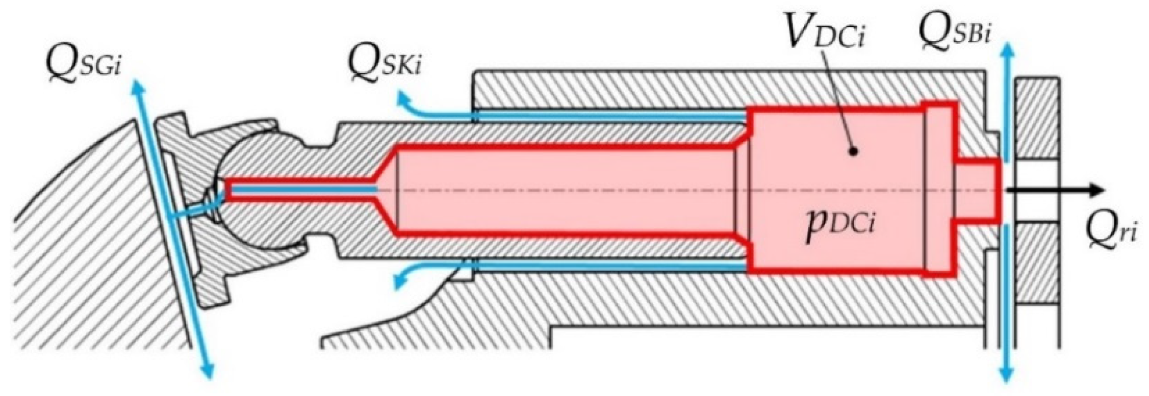
Energies 12 03096 g001
Figure 2. The schema of a displacement chamber.
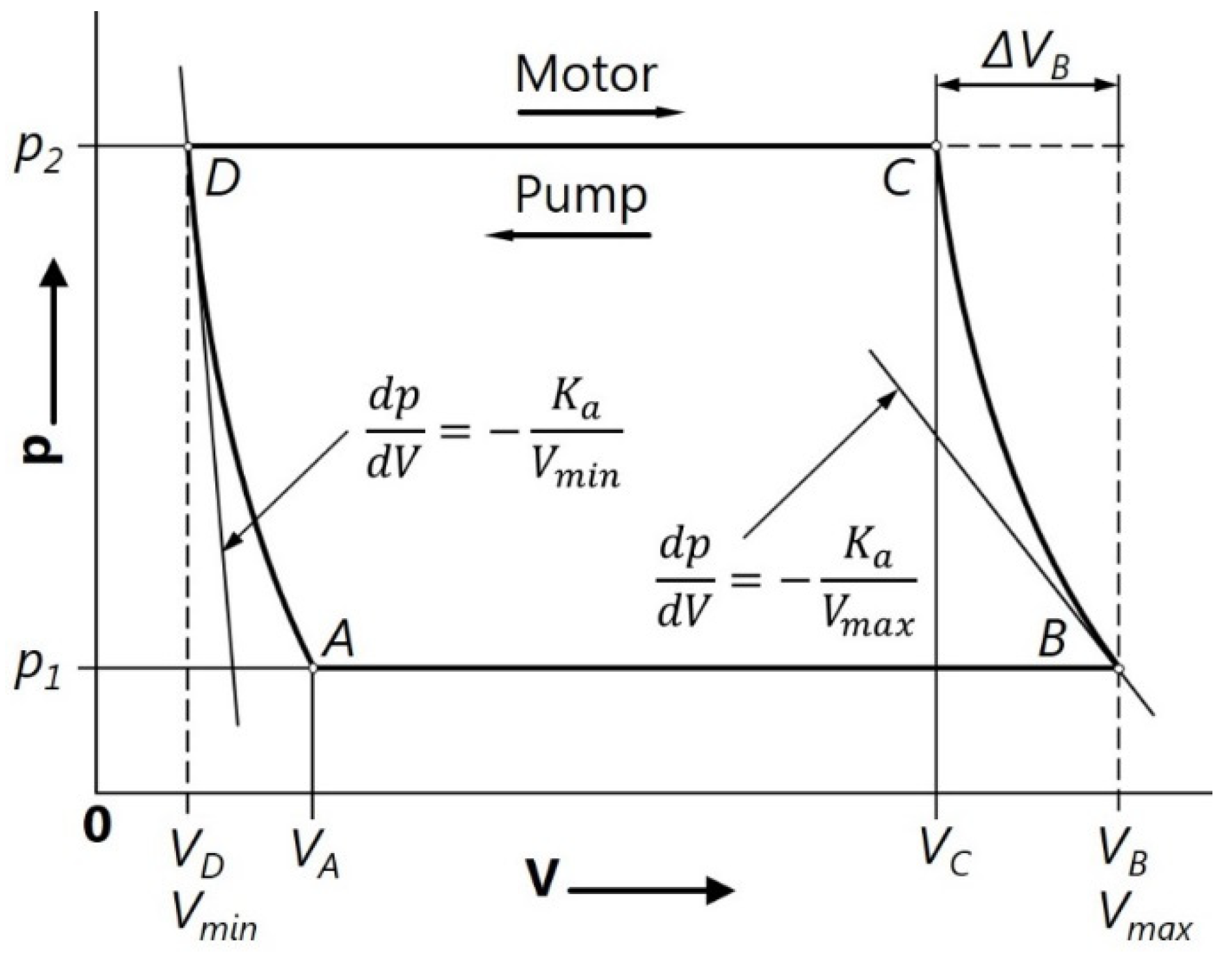
Energies 12 03096 g002
Figure 3. Diagram of an ideal displacement machine with a compressible fluid.
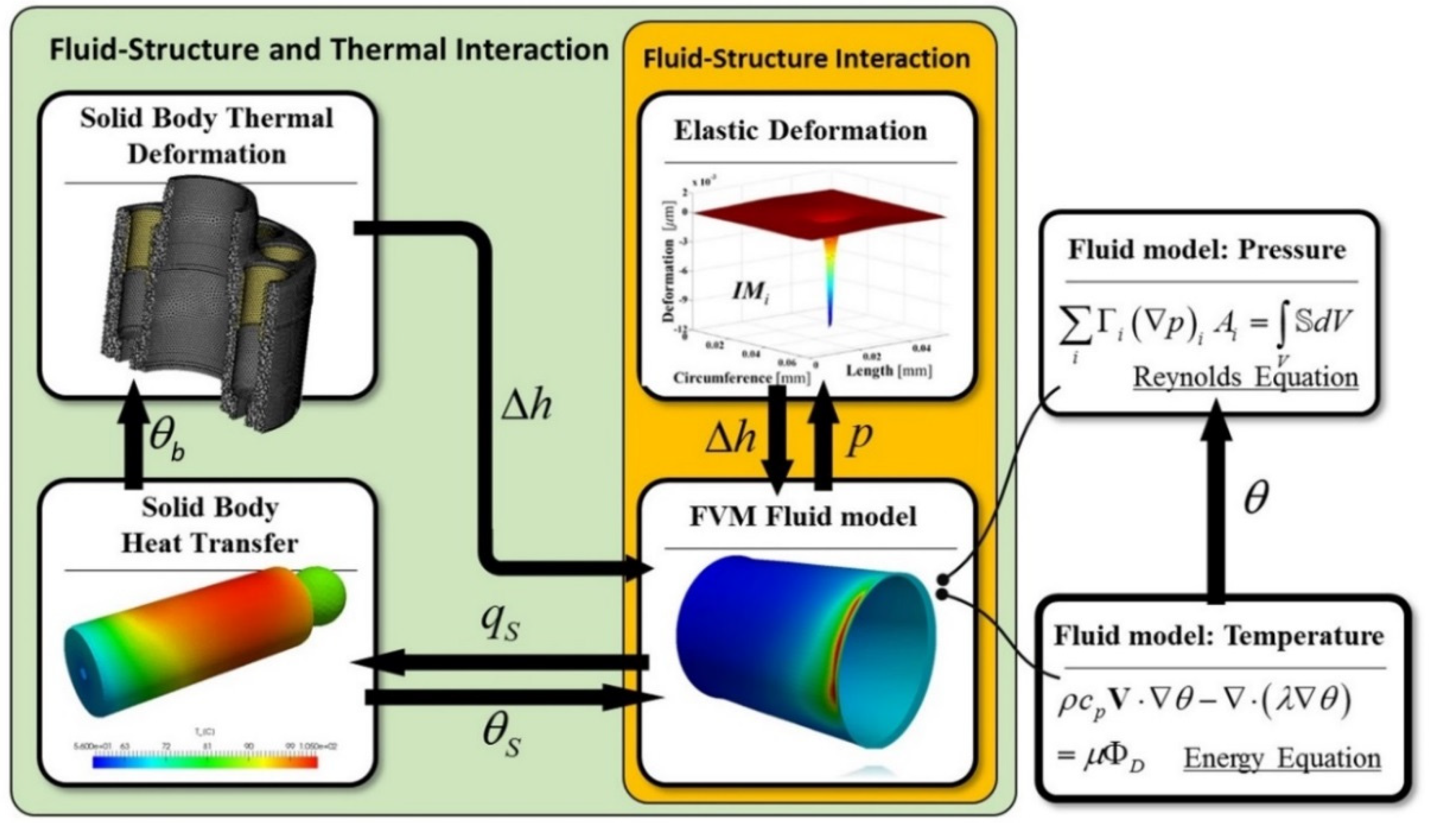
Energies 12 03096 g003
Figure 4. Structure of the simulation model for the prediction of lubricating interface performance.
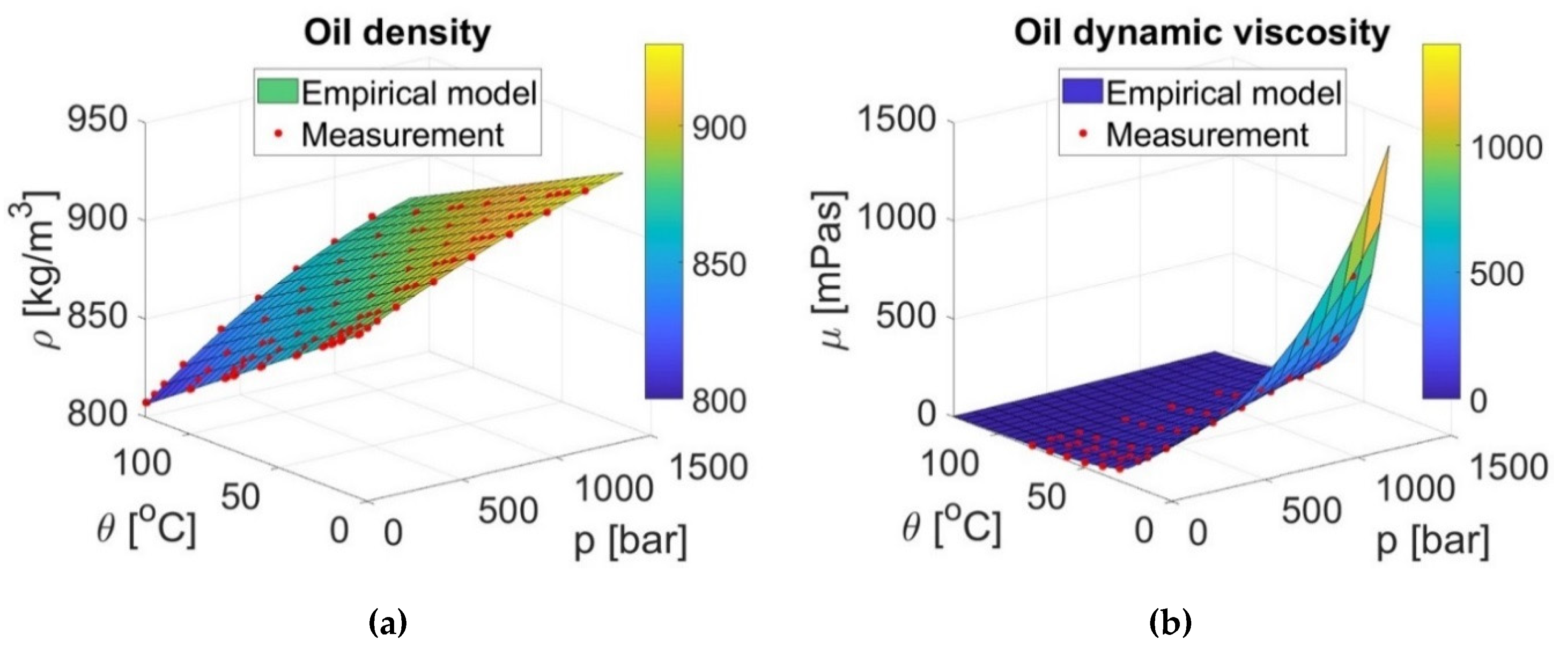
Energies 12 03096 g004
Figure 5. (a) Dependence of the density on the pressure and temperature for the oil an ISO 46 viscosity grade; (b) dependence of the viscosity on the pressure and temperature for the oil an ISO 46 viscosity grade.
Energies 12 03096 g005
Figure 6. Implementation of the pressure transducer into the cylinder block.
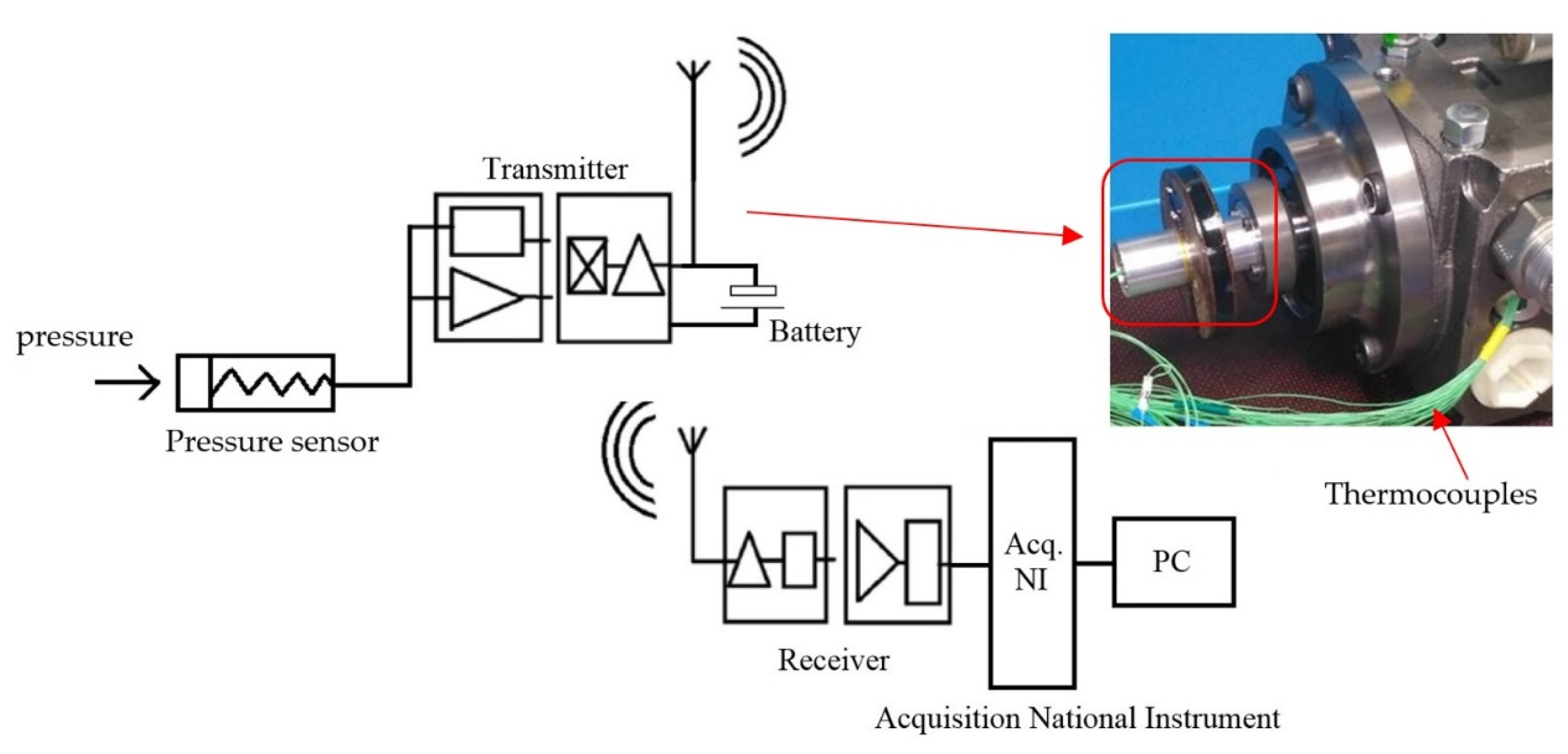
Energies 12 03096 g006
Figure 7. The principle schema of telemetry system and its installation on the pump.
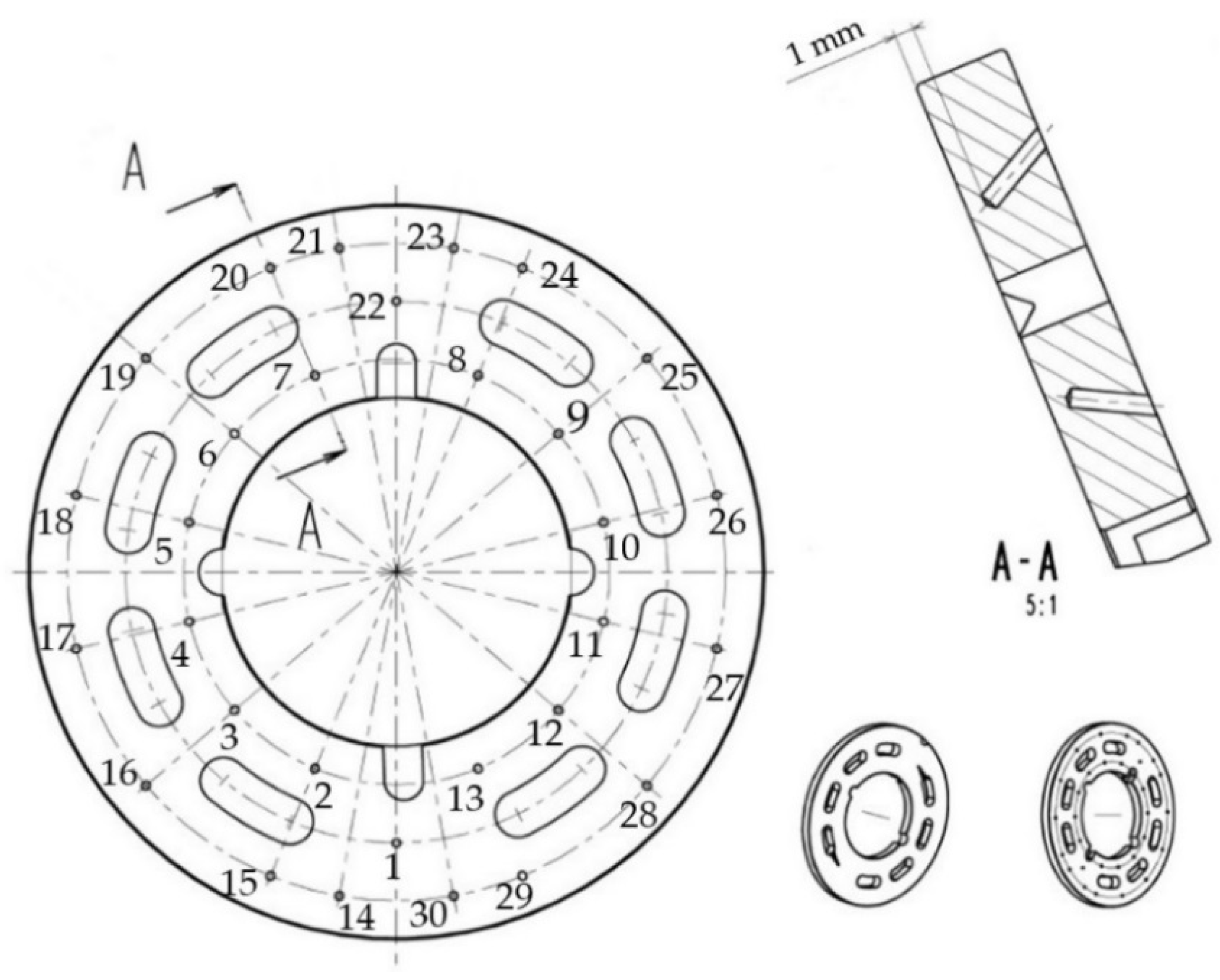
Energies 12 03096 g007
Figure 8. Position of the thermocouples in the valve plate.
Energies 12 03096 g008
Figure 9. Valve plate in the end case of the pump.
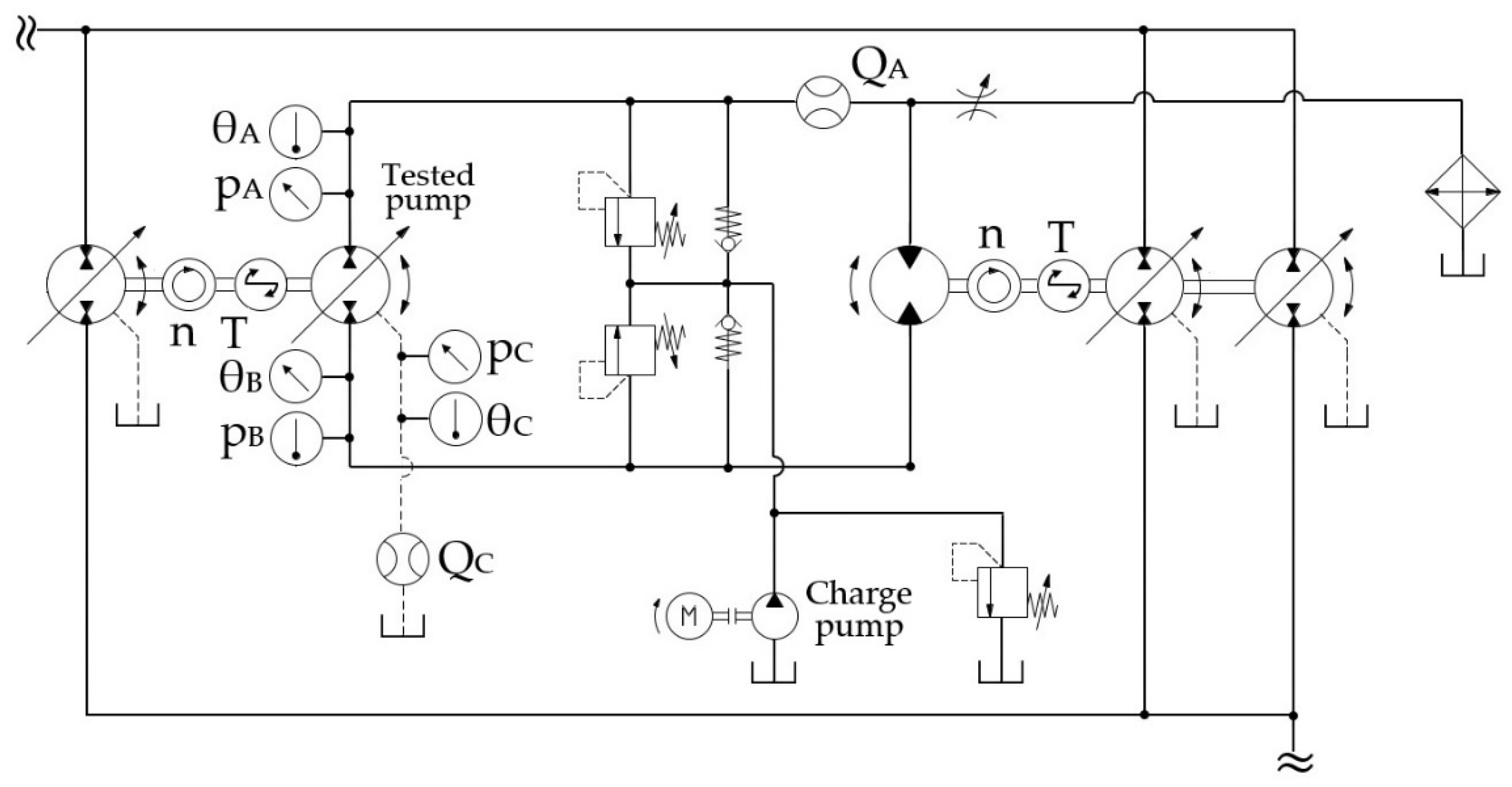
Energies 12 03096 g009
Figure 10. Hydraulic schematic of the test rig.
Energies 12 03096 g010
Figure 11. Prediction vs. measurement; displacement chamber pressure.
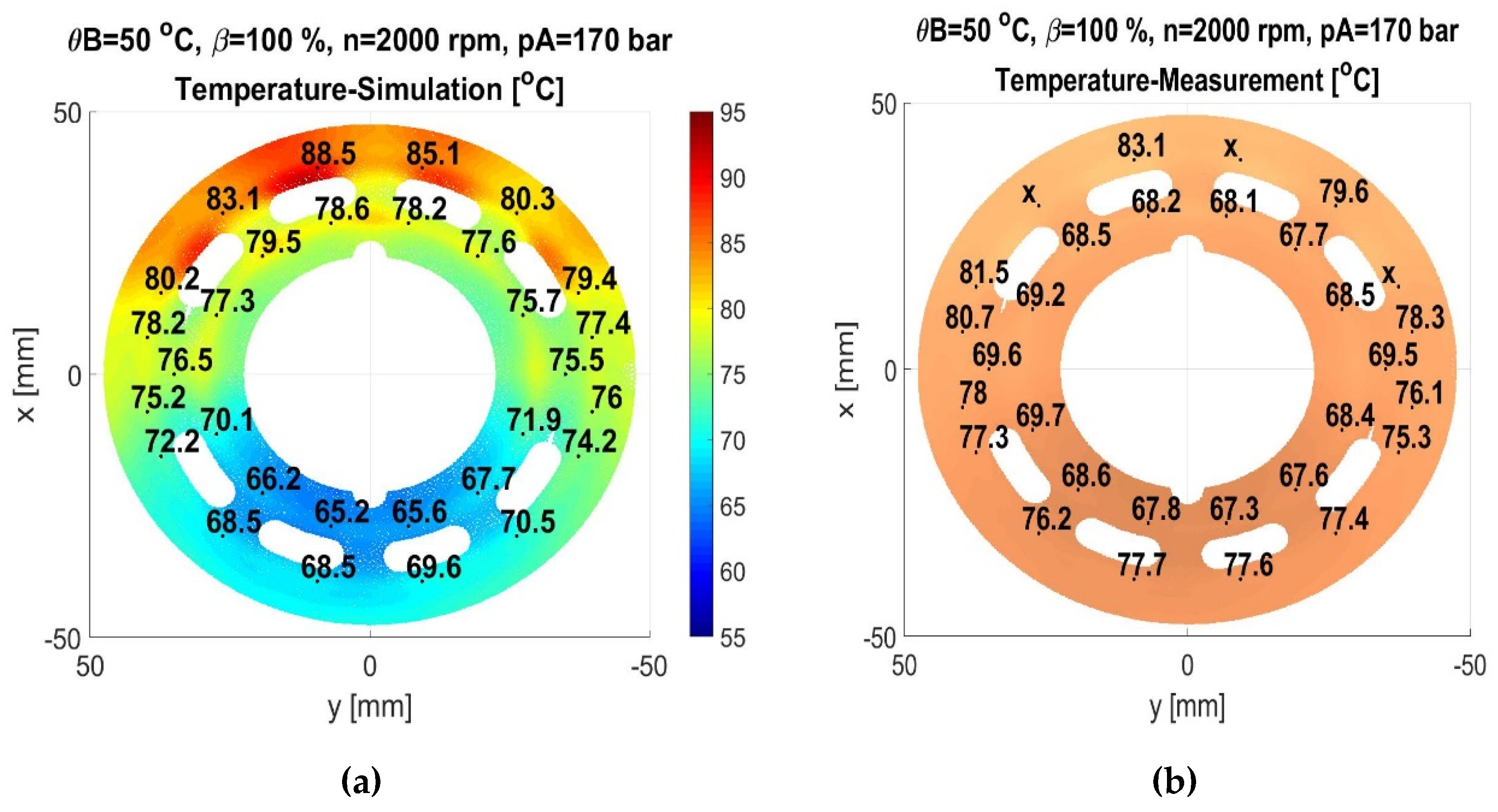
Energies 12 03096 g011
Figure 12. (a) Simulated temperature of valve plate; (b) measured temperature of valve plate.
Energies 12 03096 g012
Figure 13. (a) Difference between simulation and measurement at high power operating condition; (b) difference between simulation and measurement at low power operating condition.
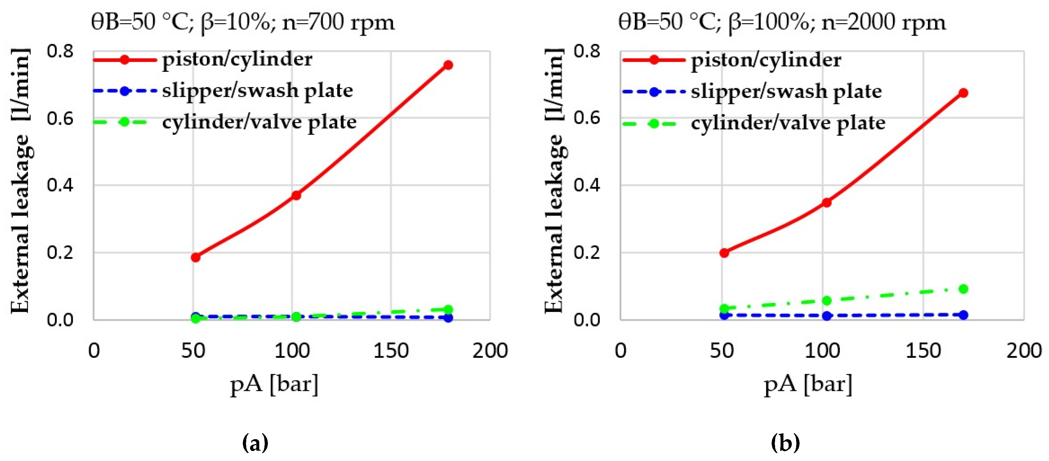
Energies 12 03096 g013
Figure 14. (a) Prediction of the leakage flow through the individual lubricating interfaces at low power operating condition; (b) prediction of the leakage flow through the individual lubricating interfaces at high power operating condition.
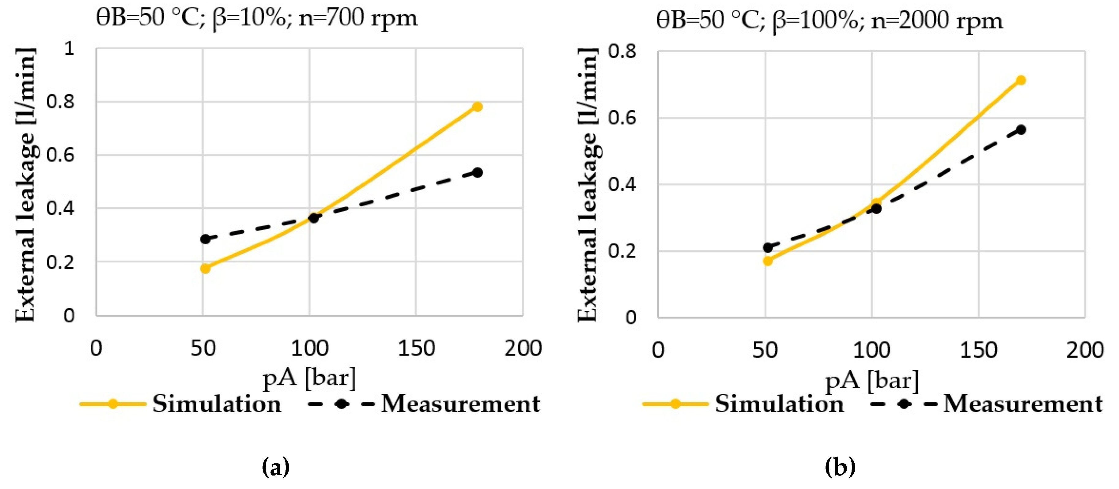
Energies 12 03096 g014
Figure 15. (a) Prediction vs. measurement; total external leakage of the pump at low power operating condition; (b) prediction vs. measurement; total external leakage of the pump at high power operating condition.
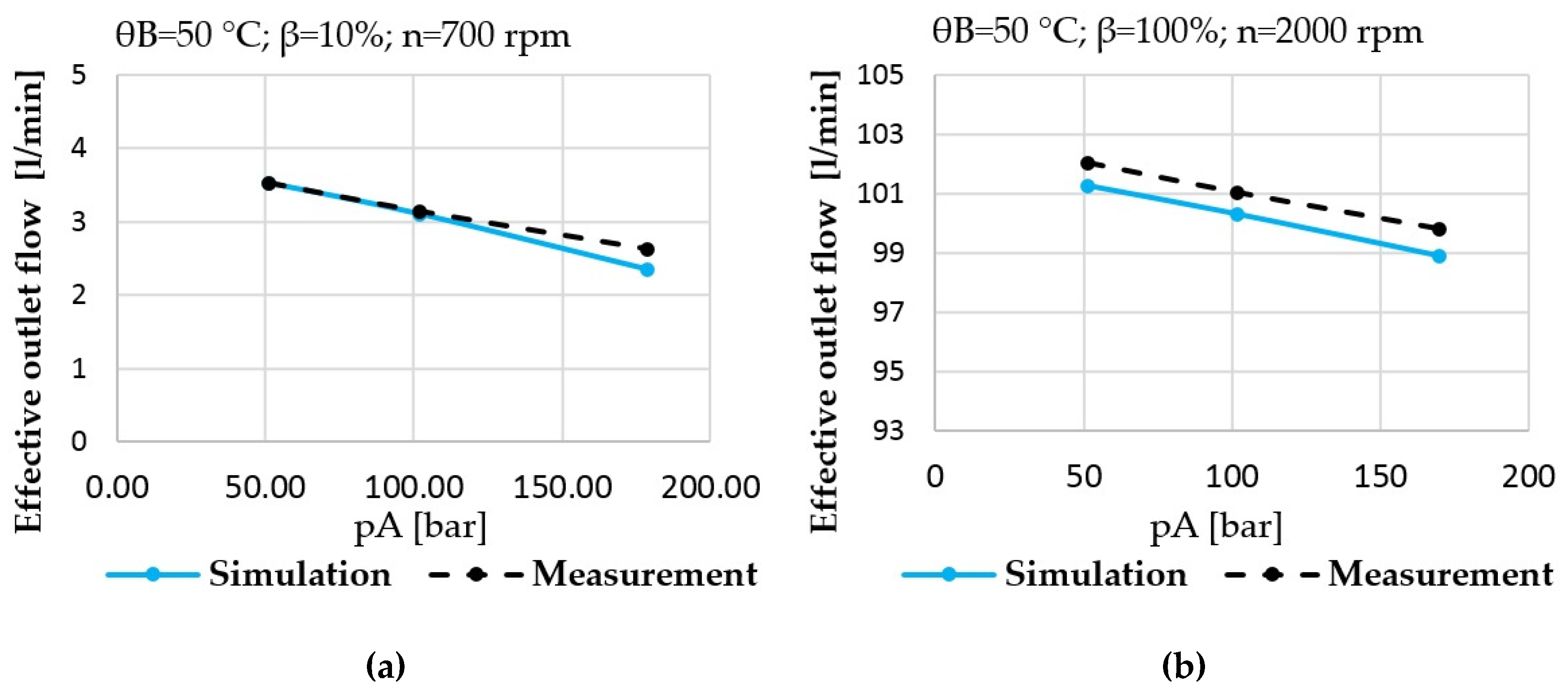
Energies 12 03096 g015
Figure 16. (a) Prediction vs. measurement; effective outlet flow of the pump at low power operating condition; (b) prediction vs. measurement; effective outlet flow of the pump at high power operating condition.
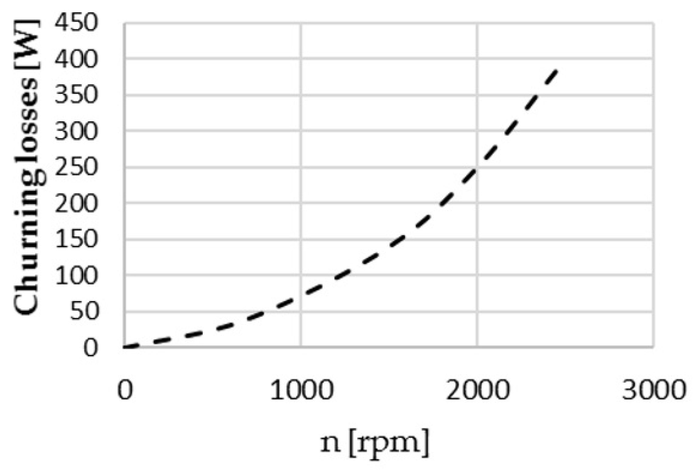
Energies 12 03096 g016
Figure 17. Churning losses of a 52 cc S-APP.
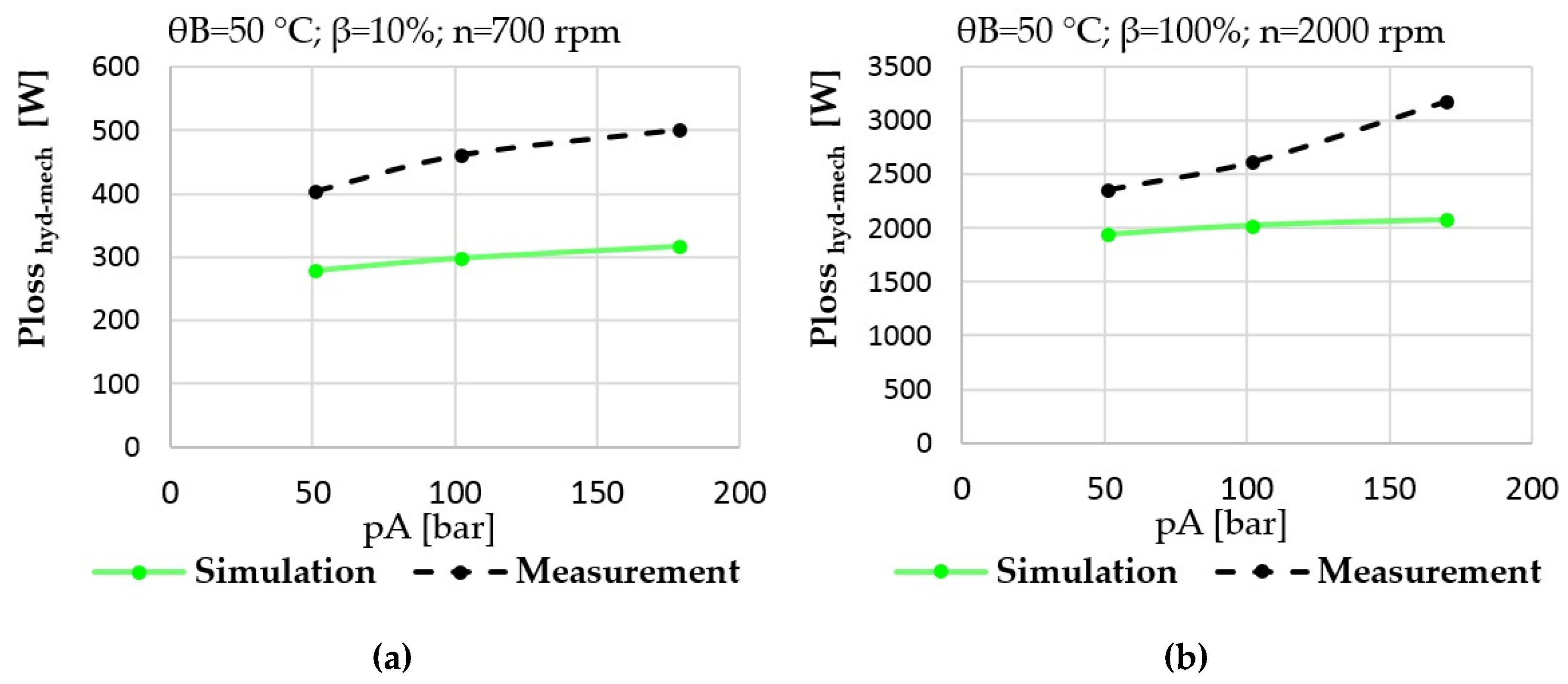
Energies 12 03096 g017
Figure 18. (a) Prediction vs. measurement; hydraulic-mechanical losses of the pump at low power operating condition; (b) prediction vs. measurement; hydraulic-mechanical losses of the pump at high power operating condition.
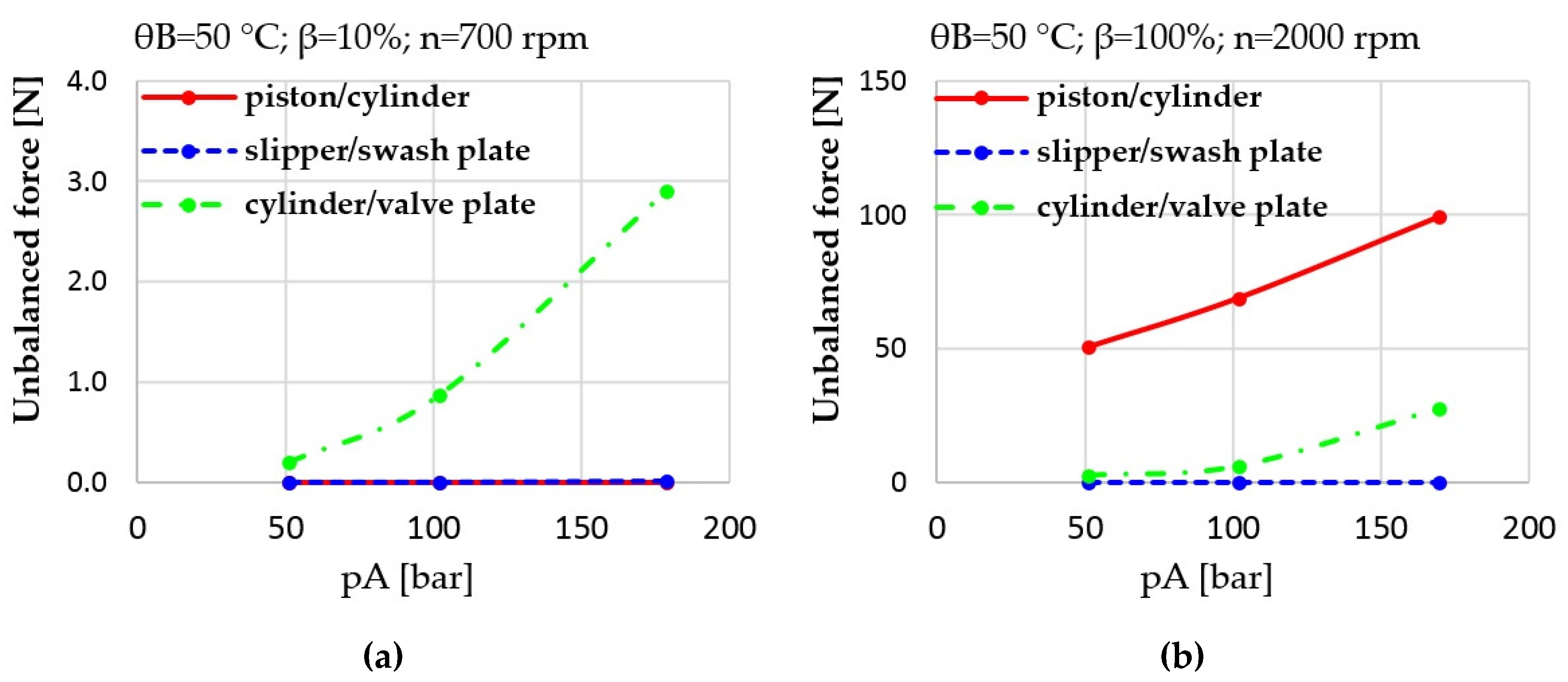
Energies 12 03096 g018
Figure 19. (a) Unbalanced forces in the individual lubricating interfaces at low power operating condition; (b) unbalanced forces in the individual lubricating interfaces at high power operating condition.
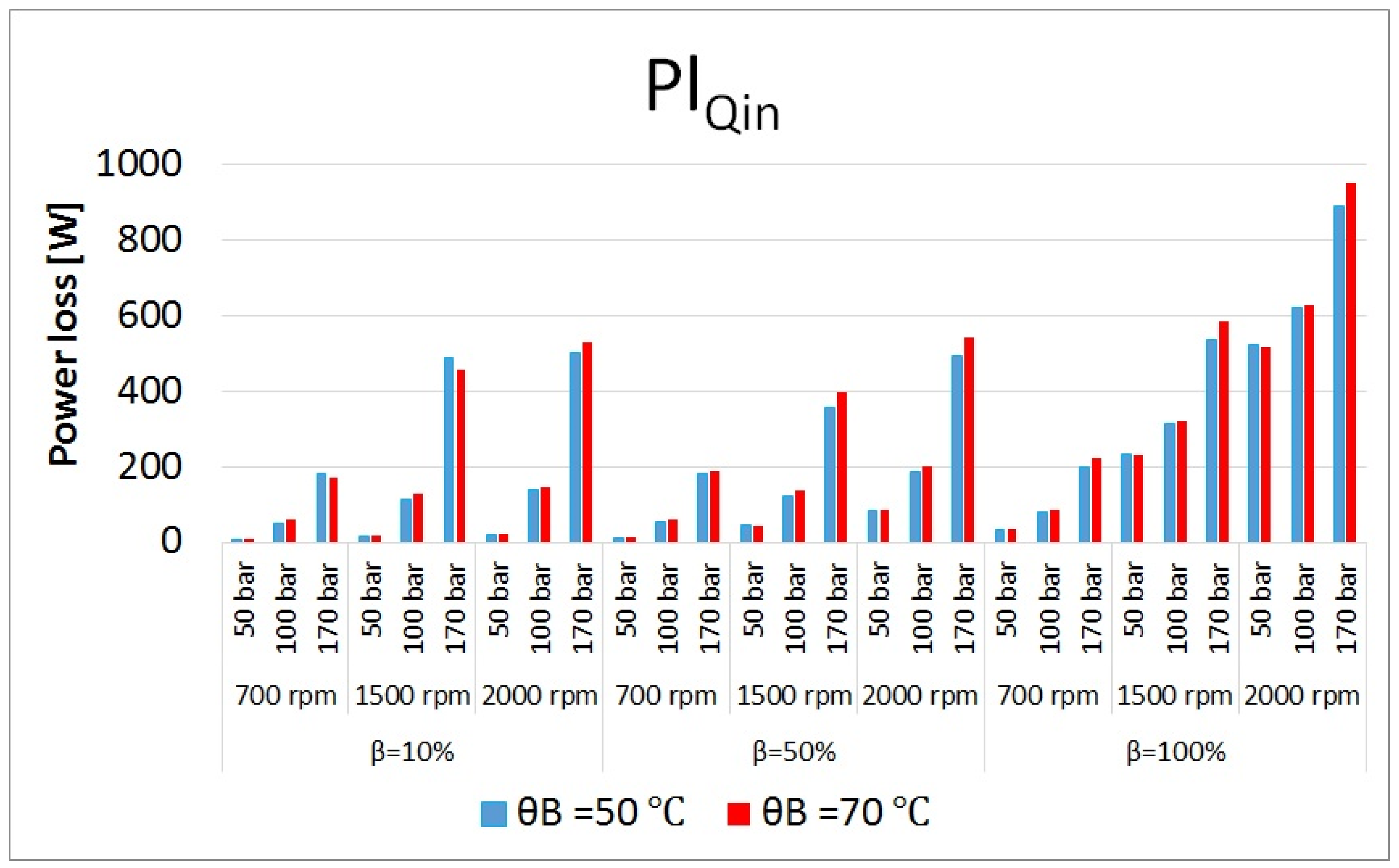
Energies 12 03096 g019
Figure 20. Power losses due to internal leakage at different operating conditions.
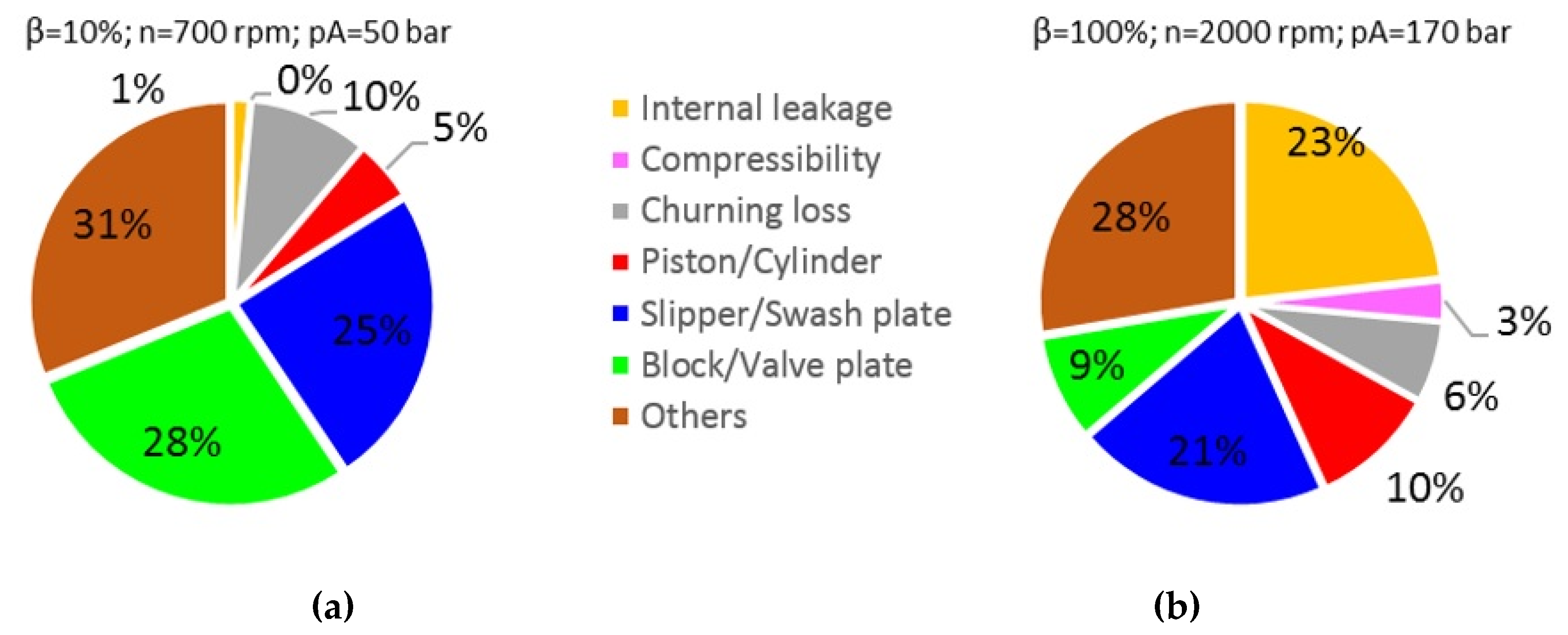
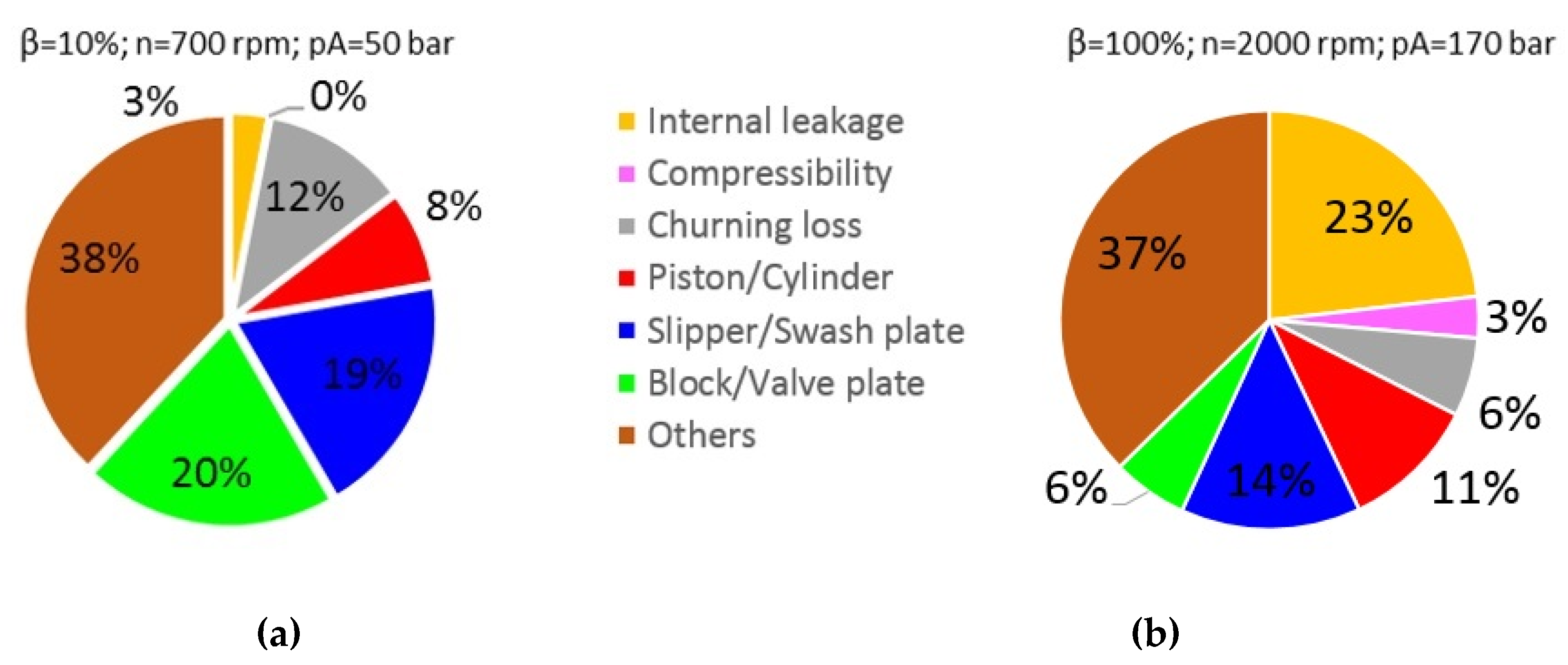
Energies 12 03096 g020
Figure 21. (a) Distribution of power losses at low power operating condition and θB = 50 °C; (b) distribution of power losses at high power operating condition and θB = 50 °C.
Energies 12 03096 g021
Figure 22. (a) Distribution of power losses at low power operating condition and θB = 70 °C; (b) distribution of power losses at high power operating condition and θB = 70 °C.
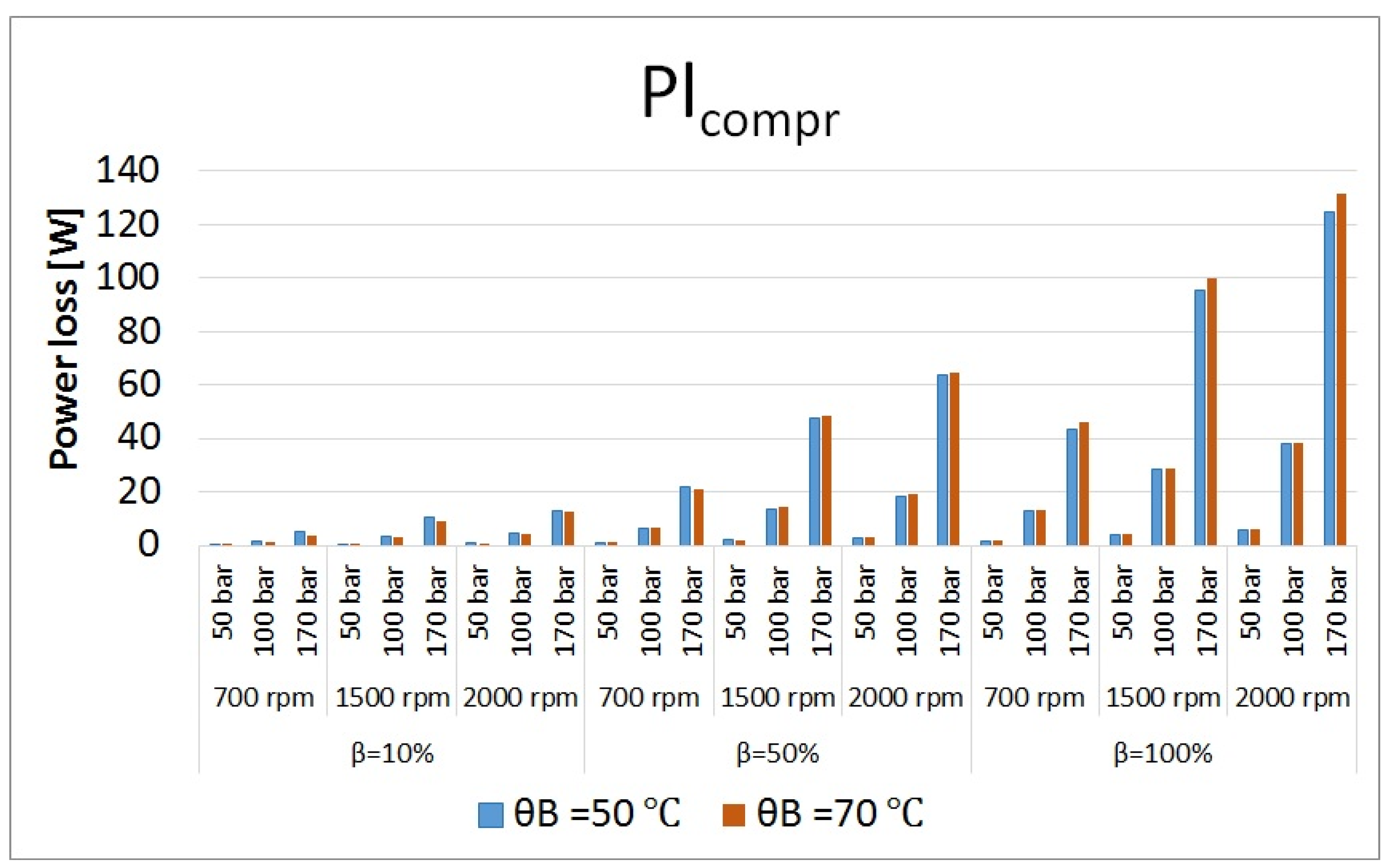
Energies 12 03096 g022
Figure 23. Compression power losses at different operating conditions.
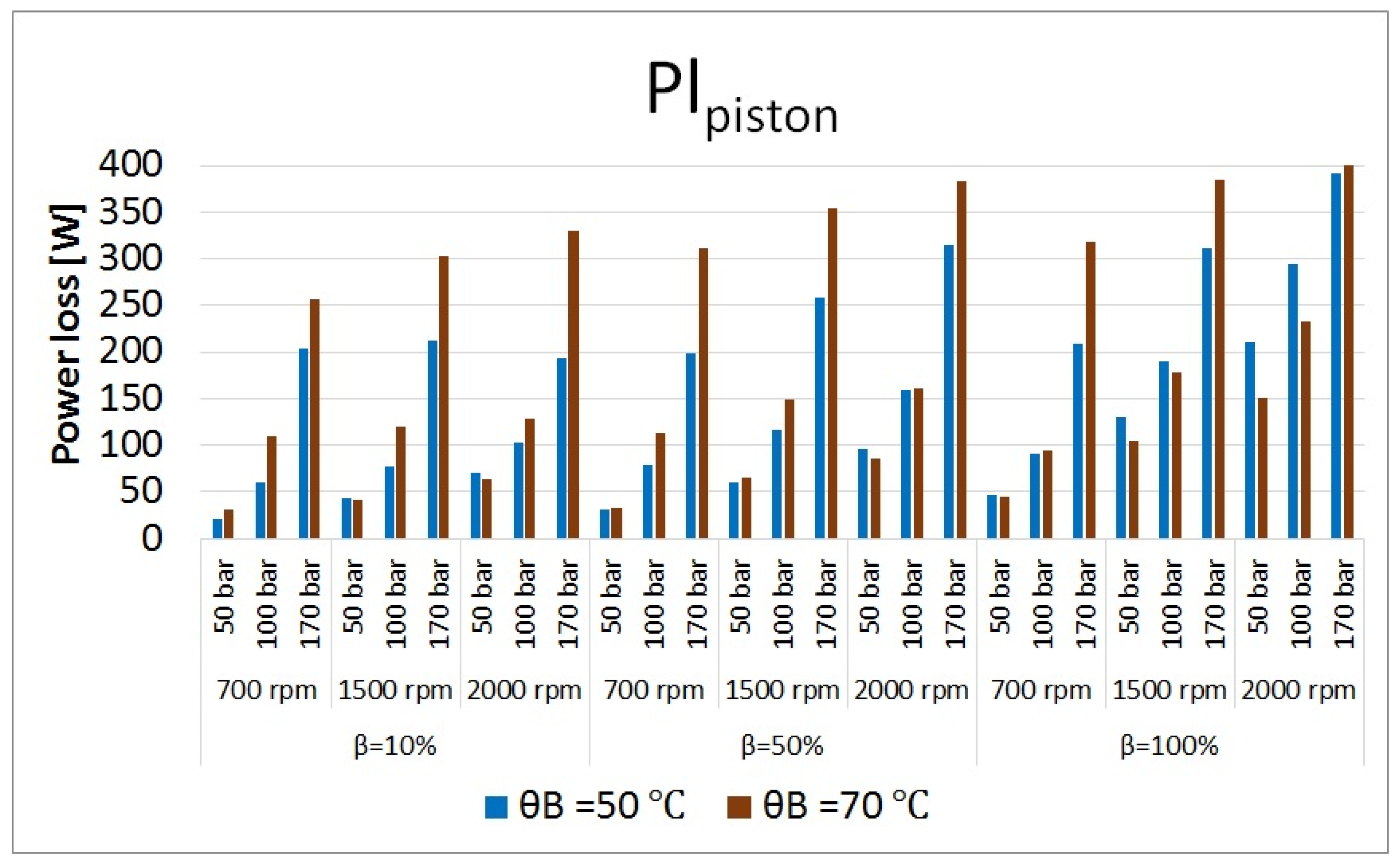
Energies 12 03096 g023
Figure 24. Total power losses in piston/cylinder bore interfaces at different operating conditions.
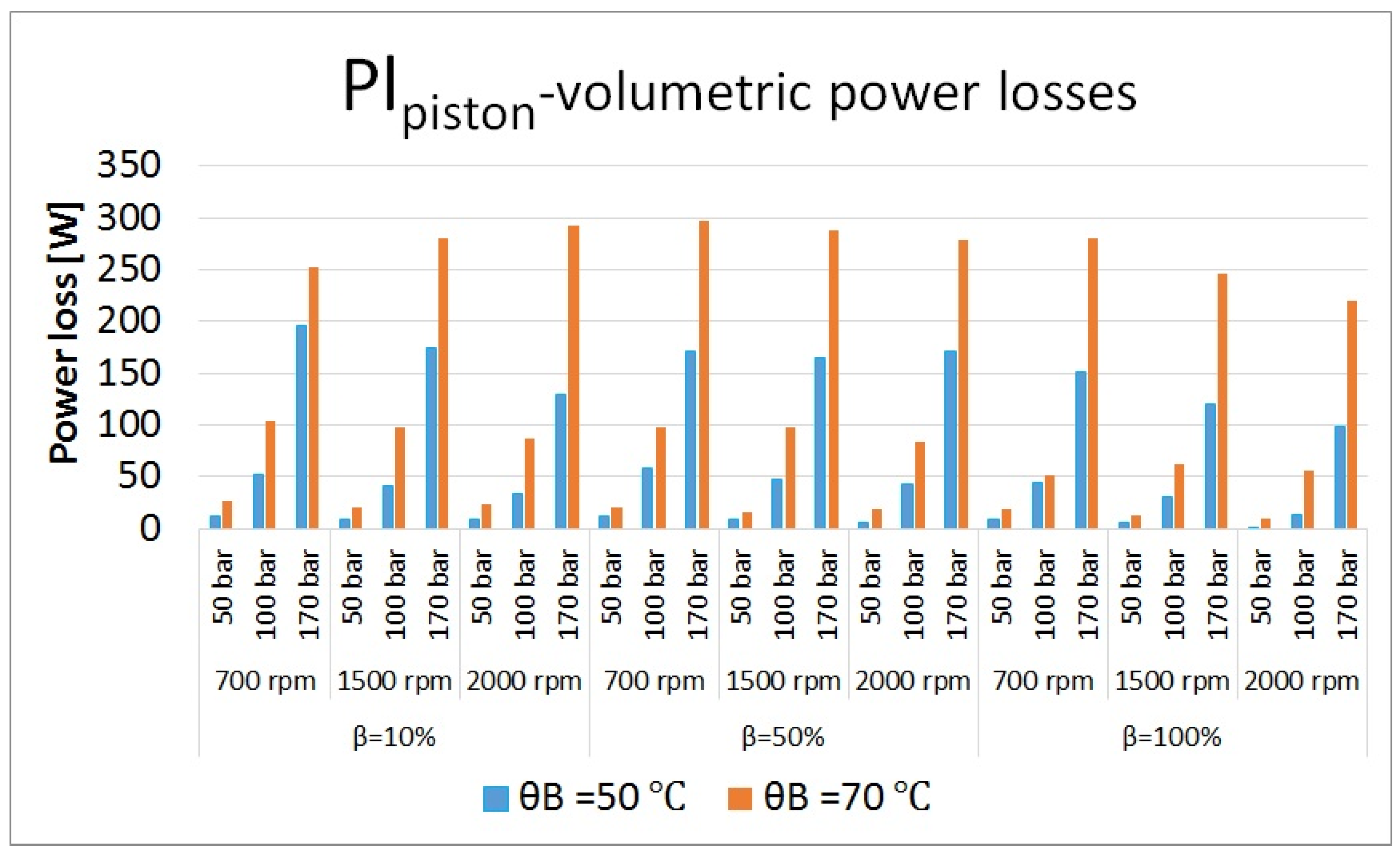
Energies 12 03096 g024
Figure 25. Volumetric power losses in piston/cylinder bore interfaces at different operating conditions.
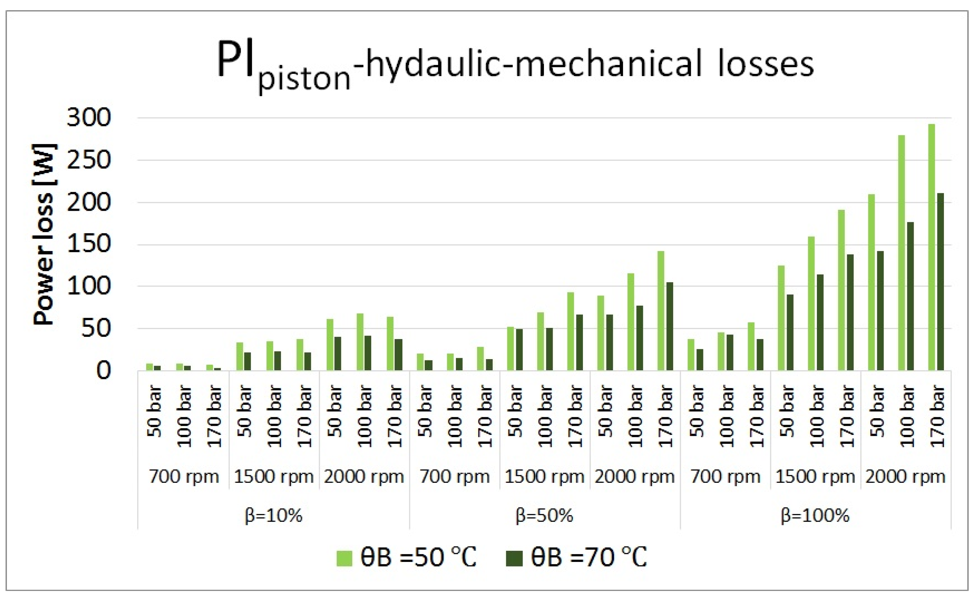
Energies 12 03096 g025
Figure 26. Hydraulic-mechanical losses in piston/cylinder bore interfaces at different operating conditions.
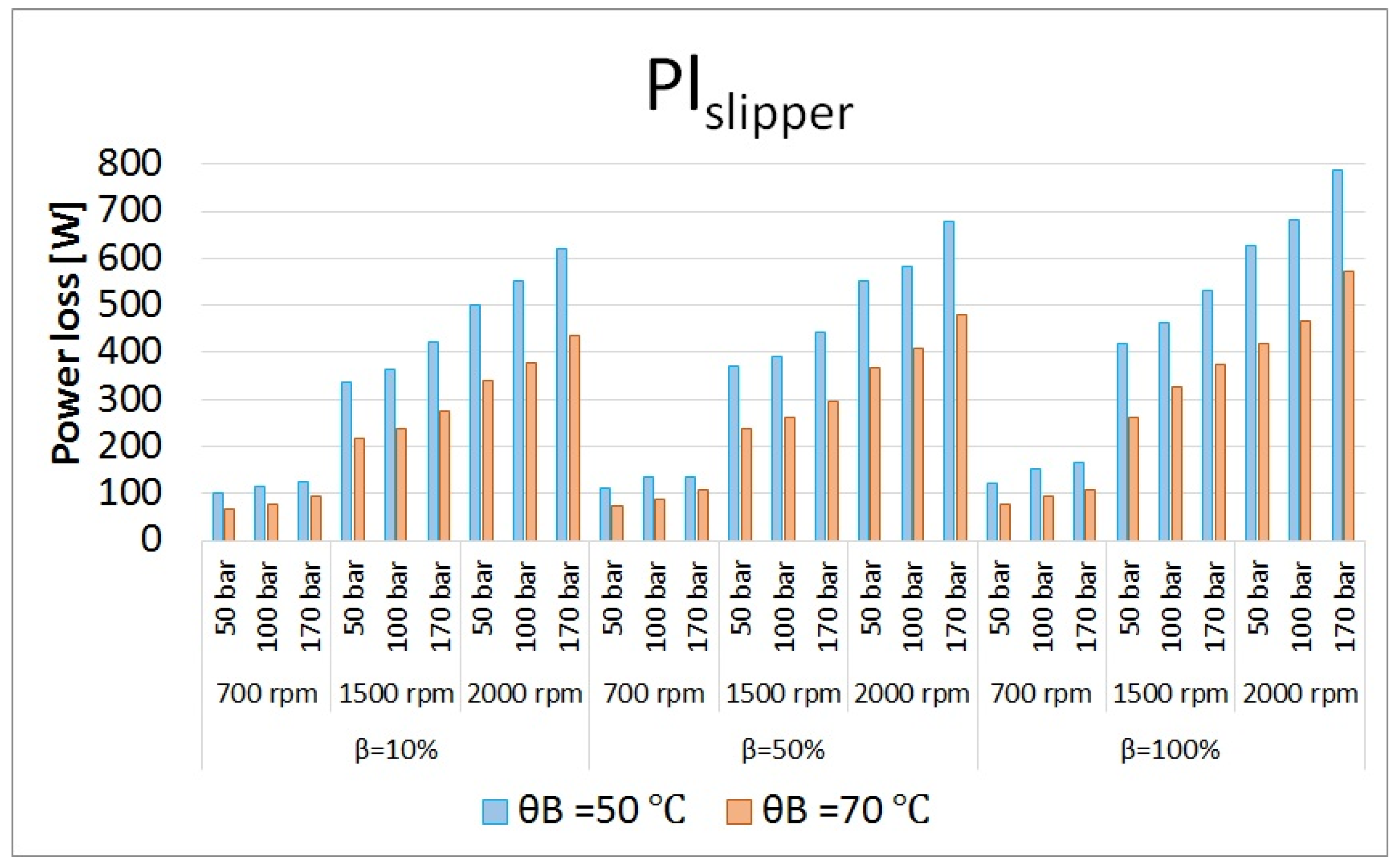
Energies 12 03096 g026
Figure 27. Total power losses in slipper/swash plate interface at different operating conditions.
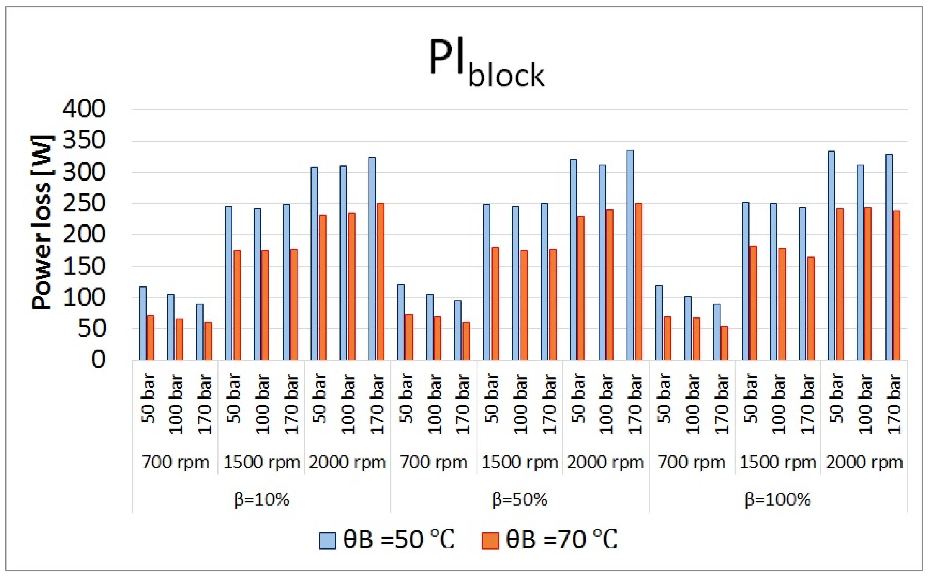
Energies 12 03096 g027
Figure 28. Total power losses in cylinder block/valve plate interface at different operating conditions.
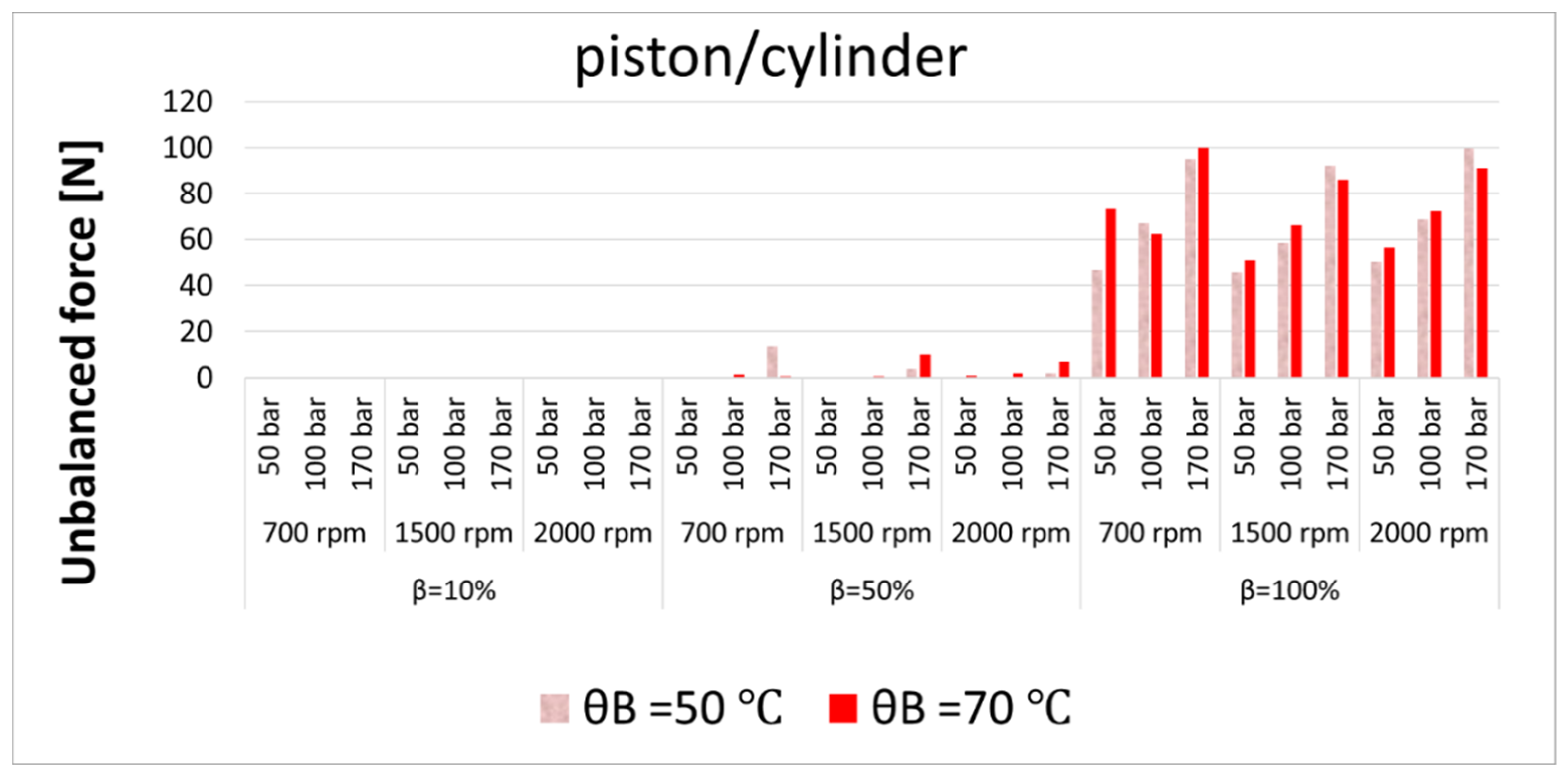
Energies 12 03096 g028
Figure 29. Unbalanced forces in the piston/cylinder interfaces at different operating conditions.
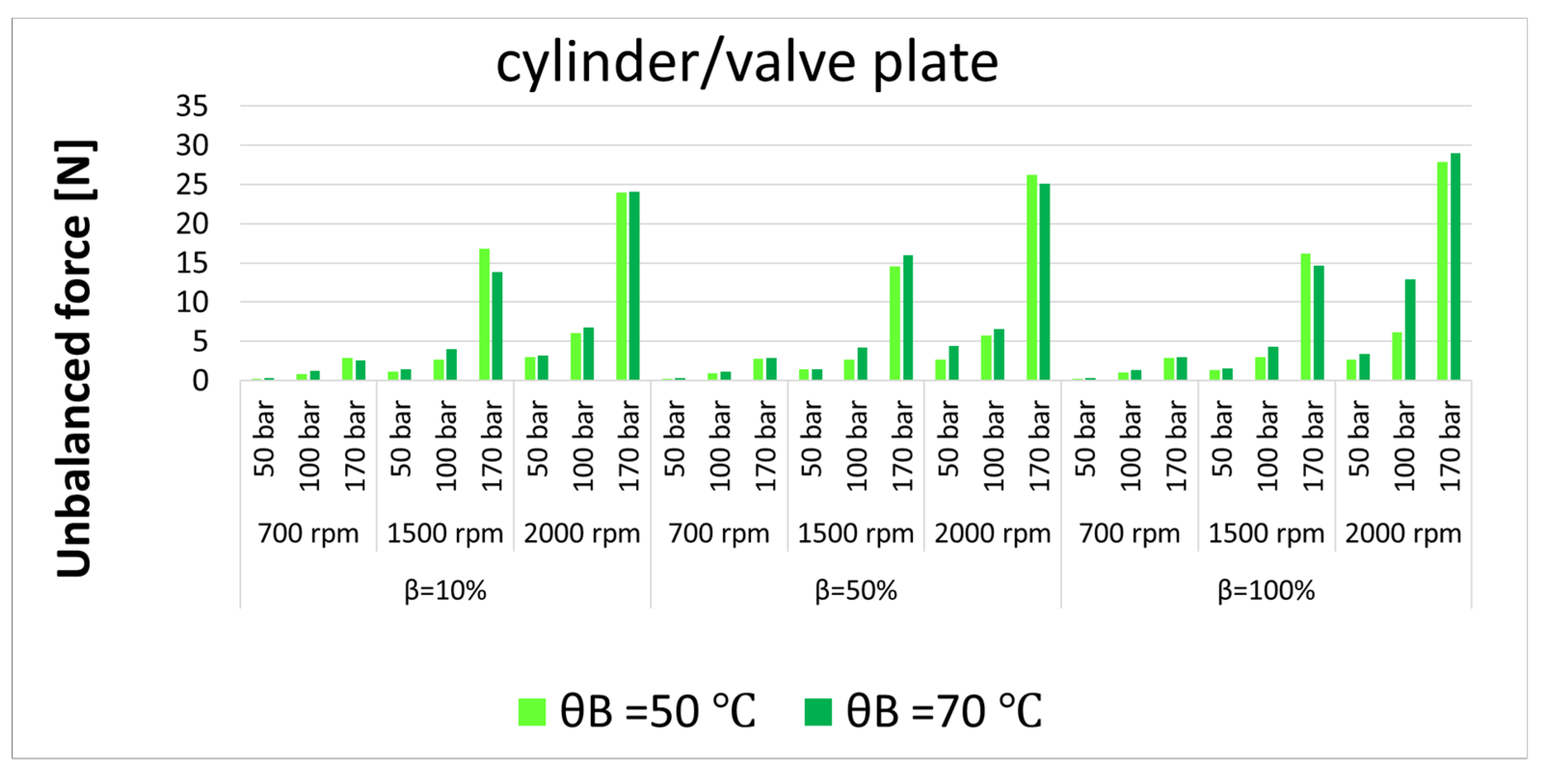
Energies 12 03096 g029
Figure 30. Unbalanced forces in the cylinder/valve plate interfaces at different operating conditions.
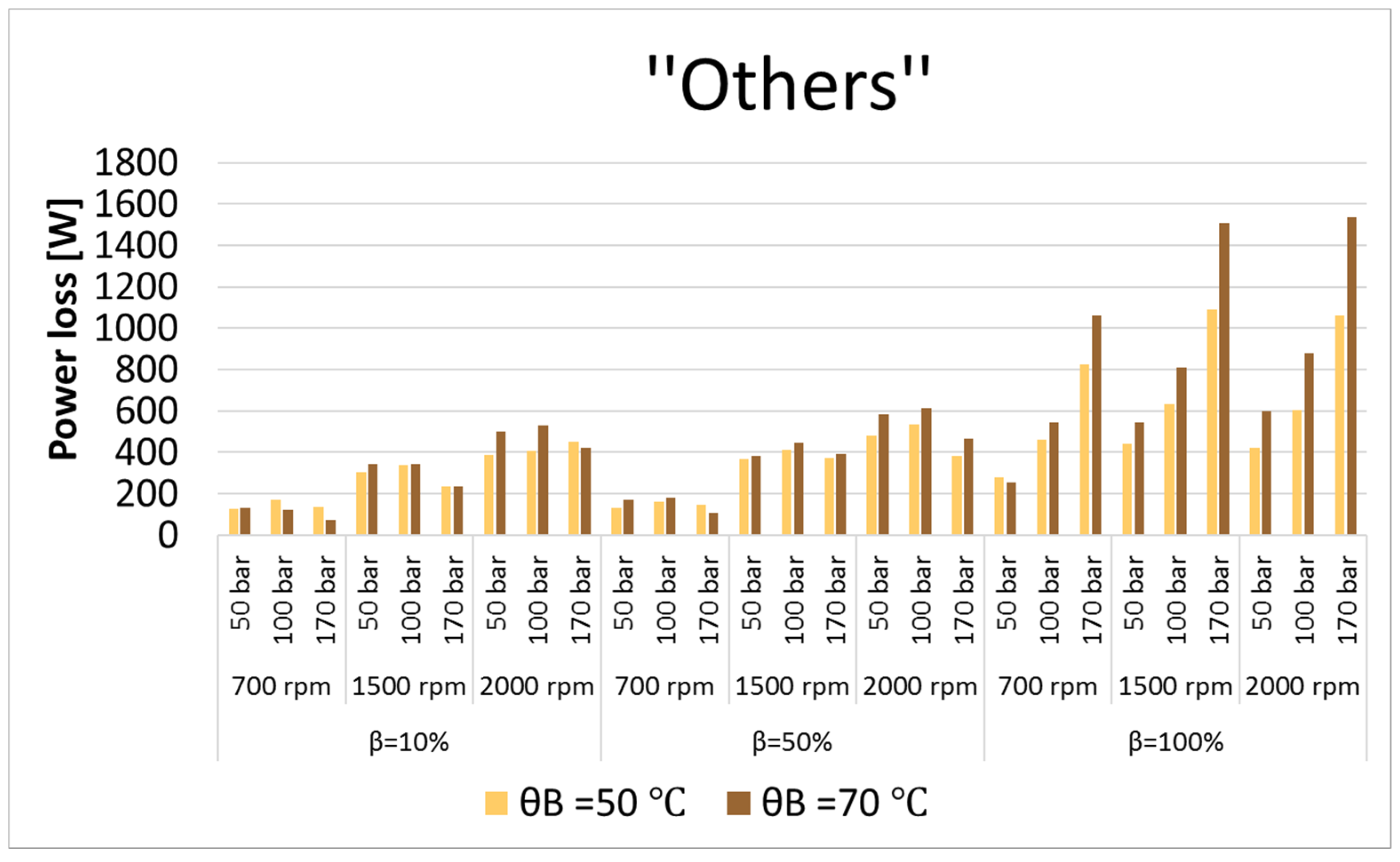
Energies 12 03096 g030
Figure 31. Undefined losses at different operating conditions.
Energies 12 03096 g031
Table 1. Data of the reference S-APP.
ParameterValueUnit
Number of pistons 9(-)
Max displacement 52(cc/rev)
Speed ratingsmin700(rpm)
max3400
System pressurerated300(bar)
max400
min low loop15
Table 2. Steady-state measurement sensors.
SensorParameterSpecificationAccuracy
T, ntorque, speedHMB T40B/500 Nmclass 0.05
QAflowKEM SRZ 400 KL+/−0.31%
QCcase flowKEM SRZ 100 KL+/−0.36%
pA, pBpressure in A, B lineHBM P3ICP/500 bar+/−0.033%
pCcase pressureHBM P3ICP/50 bar+/−0.092%
θA, θB, θCtemperatureOmega K Type Thermocouple+/−1.1 °C
θivalve plate temperatureOmega K Type Thermocouple+/−1.1 °C
pDCdispl. chamber pressureKistler 603CA+/−0.04%
φshaft angular positionROS-W 1906009; 1–250,000 RPMNA
Table 3. The operating conditions considered in this study.
Inlet Temperature θBDisplacement βSpeed nOutlet Port Pressure pA
50 °C10%700 rpm50 bar
70 °C50%1500 rpm100 bar
-100%2000 rpm170 bar
Table 4. Average error of the valve plate temperature.
Average Error (°C)
βnpAθB = 50 °CθB = 70 °C
10%700 rpm50 bar2.0 1.3
100 bar1.31.1
170 bar2.41.6
1500 rpm50 bar3.73.0
100 bar3.72.9
170 bar3.62.5
2000 rpm50 bar4.52.1
100 bar4.63.4
170 bar4.94.0
50%700 rpm50 bar2.41.2
100 bar1.31.1
170 bar1.51.5
1500 rpm50 bar4.13.4
100 bar3.83.1
170 bar3.52.8
2000 rpm50 bar5.44.1
100 bar4.84.2
170 bar5.14.2
100%700 rpm50 bar1.91.1
100 bar1.52.3
170 bar3.64.5
1500 rpm50 bar4.53.5
100 bar3.72.7
170 bar3.83.3
2000 rpm50 bar5.94.7
100 bar4.74.2
170 bar4.34.1
Table 5. Distribution of power losses in the S-APP a 52 cc size; θB = 50 °C.
Power Losses (W)
βnHPPltotalPlQinPlcomprPlchurningPlpistonPlslipperPlblock‘’Others’’
10%700 rpm50 bar413.660.340.020.5101.2116.8128.8
100 bar537.247.81.540.060.3113.2105.7168.6
170 bar782.1183.24.940.0203.7124.589.9135.9
1500 rpm50 bar1084.116.10.6140.042.3337.0245.9302.2
100 bar1279.1115.03.1140.077.0364.1241.4338.5
170 bar1755.6490.910.5140.0211.8420.6248.7233.1
2000 rpm50 bar1536.918.60.8250.070.8500.7308.2387.8
100 bar1767.0139.44.4250.0102.2552.3310.2408.4
170 bar2352.4501.713.2250.0193.7619.7324.5449.6
50%700 rpm50 bar452.312.21.040.031.8112.8120.5134.0
100 bar581.555.06.340.079.8135.2104.5160.7
170 bar819.1182.622.140.0198.4134.595.2146.3
1500 rpm50 bar1232.443.52.1140.060.8371.6248.1366.3
100 bar1439.2121.513.6140.0116.4390.9244.5412.4
170 bar1868.8357.647.5140.0258.4443.8249.7371.9
2000 rpm50 bar1788.484.62.9250.095.9552.0320.8482.3
100 bar2040.7184.118.3250.0158.6583.9311.4534.4
170 bar2519.7492.663.9250.0313.9679.4335.3384.6
100%700 rpm50 bar643.933.31.840.046.9121.0119.4281.5
100 bar936.179.813.140.090.8151.0102.6458.8
170 bar1570.0197.343.440.0209.3165.689.3825.1
1500 rpm50 bar1615.8233.64.1140.0130.0417.6251.4439.0
100 bar2018.0312.428.2140.0190.6463.4249.5634.0
170 bar2944.6534.795.4140.0311.3531.1243.81088.4
2000 rpm50 bar2372.8524.65.6250.0209.9627.8334.3420.6
100 bar2804.9621.738.3250.0294.2682.9312.1605.7
170 bar3828.8888.4124.4250.0391.8786.6328.31059.3
Table 6. Distribution of power losses in the S-APP a 52 cc size; θB = 70 °C.
Power losses (W)
βnHPPltotalPlQinPlcomprPlchurningPlpistonPlslipperPlblock‘’Others’’
10%700 rpm50 bar351.810.40.340.031.967.170.3131.8
100 bar473.359.31.540.0109.377.465.9119.8
170 bar698.3169.73.940.025694.860.473.5
1500 rpm50 bar935.117.10.6140.042.1216.5175.4343.4
100 bar1148.3130.03.2140.0120.2238.5174.5341.9
170 bar1595.8458.69.2140.0302.4273.8177.1234.7
2000 rpm50 bar1404.320.50.7250.062.8338.9231.6499.8
100 bar1671.0146.14.4250.0129.3379.2234.4527.6
170 bar2232.2530.812.7250.0330.8436.5249.9421.6
50%700 rpm50 bar403.013.21.040.032.973.272.4170.4
100 bar559.462.36.540.0113.285.869.4182.2
170 bar834.5189.620.940.0311.1106.360.0106.6
1500 rpm50 bar1049.644.32.1140.065236.1180.2381.9
100 bar1326.5138.014.5140.0148.6263.0176.0446.4
170 bar1803.5397.348.5140.0354.7295.7176.2391.0
2000 rpm50 bar1603.384.92.8250.085.8367.9230.2581.6
100 bar1890.6199.719.0250.0161.1406.8240.8613.2
170 bar2437.8540.864.8250.0383.6479.8251.1467.8
100%700 rpm50 bar524.834.12.040.044.477.769.7256.9
100 bar936.383.913.340.093.992.966.8545.6
170 bar1851.2222.746.240.0317.7108.054.71061.8
1500 rpm50 bar1468.4232.84.5140.0103.8261.3182.5543.4
100 bar1982.0320.728.9140.0177.2327.0178.3809.8
170 bar3255.5585.0100.0140.0383.9374.9164.71507.0
2000 rpm50 bar2182.1517.65.8250.0151.2417.4241.9598.2
100 bar2736.4627.038.6250.0232.7467.6244.1876.4
170 bar4112.5953.6131.3250.0431.2571.8239.11535.4

