Evaluation of Accommodation Capability for Electric Vehicles of a Distribution System Considering Coordinated Charging Strategies

Abstract

In recent years, the ever-increasing charging demand of electric vehicles (EVs) imposes challenges on both power supply security and reliability in the distribution system. In this paper, an EV accommodation capability evaluation model of a distribution system, with high penetrations of flexible resources, is established. Firstly, according to the actual classifications of EVs and transportation rules, a Monte Carlo simulation is used to simulate the charging behaviors of EVs so as to obtain the relevant parameters of EV charging. Then, a coordinated charging optimization model for various types of EVs is proposed based on the charging characteristics of EVs. The presented model comprises a mixed-integer linear programming problem and a constrained optimization problem which are respectively solved by CPLEX (the Simplex method implemented in the °C programming language) and the particle swarm optimization (PSO) algorithm. Last of all, a real-life distribution system in the coastal areas of China is served for demonstrating the feasibility and efficiency of the proposed approach. Moreover, the impacts of flexible resources, distribution network zoning rules, and EV growth on the EV accommodation capability of a distribution system are also discussed.

1. Introduction

The rapid development of electric vehicles (EVs) has received extensive attention [1,2,3], due to their great potential for saving energy, and reducing emissions. The ever-increasing penetration of EV charging demand has been observed in many actual power distribution systems. As a new type of load (with a high degree of uncertainty), the integration of numerous EVs could bring great challenges to the secure and economic operations of the distribution system [4,5,6]. This may result in increasing energy losses, voltage deviations, and even overloads in feeders and/or substations. The relationship among feeder losses, load factor, and load variance is explored in the context of coordinated charging of plug-in hybrid vehicles (PHEV) in Reference [1]. In Reference [7], the impacts of EV charging on power loss and the voltage threshold-crossing of the distribution network at different scales are analyzed. The impact of EV integration on the life cycles of transformers is investigated in Reference [8]. The mathematical model for harmonic evaluation of multiple EV charging machines is established in Reference [9]. Therefore, it is necessary to conduct a quantitative evaluation of the accommodation capability for EVs (ACE). At the same time, the optimized EV charging load (OECL) obtained by the coordinated charging strategies is also conducive to understanding the relationship between EV accommodation and charging load distribution.

It is generally agreed that the problems of environmental pollution and energy security can be abated by increasing the penetration level of both EVs and flexible resources, such as a variety of distributed generations (DGs) and energy storage systems (ESSs). Flexible resources on the demand side will play a pivotal role in reducing load fluctuations in the distribution system [10]. Besides, better utilization of the flexible resources on both power supply and demand sides is one approach to increase the ACE. Joint optimal scheduling of flexible resources and EVs have been investigated by a number of researchers. Simultaneous provision of interruptible loads for flexible ramping products and demand relief are considered in Reference [11]. The impact of EVs and demand response (DR) on the flexibility of a microgrid are analyzed in Reference [12]. A multi-objective optimal scheduling method for a distribution network with the integration of numerous EVs is proposed in Reference [13].

In terms of the ACE evaluation, there are mainly two types of methods. One method is to optimize the maximum ACE under the assumption of EV behaviors being guided by a smart charging strategy or a market mechanism. In Reference [14], a market mechanism that optimally allocates available charging capacity is proposed, considering the network stability and the EV owners’ individual preferences. In Reference [15], a market-based multi-agent control mechanism that takes into account the distribution transformer and voltage constraints for the EV charging is presented. A stochastic optimization-based dispatch model which is capable of handling uncertain outputs of renewable generation and PHEVs is formulated in Reference [16]. The second method investigates the ACE of a distribution system, with respect to actual charging rules and corresponding security constraints. A methodological framework is presented in Reference [17] to evaluate and maximize the ACE of a given distribution system with some statistical distributions to simulate daily travel patterns. In Reference [18], EV charging is formulated as a receding horizon optimization problem to shift EV charging to off-peak periods, taking into account the present and the ex-ante operational constraints in a distribution system. A two-stage optimization model is proposed in Reference [19] to optimize EV charging regions with consideration of actual transportation rules of EVs and the distribution network constraints in a worst-case scenario.

A zonal distribution system can be divided into several subareas with each of them aiming to supply a specific type of power load in geographic scope. Each subarea may have its own reliability standard that directly and remarkably influences the ACE. In Reference [20], the typical UK power distribution network is first divided into residential, industrial and commercial load areas, and then the relationship between different charging modes and the electricity price policies of each region is studied. The results show that the classification of load areas will improve the accuracy of the ACE assessment. On this basis, the characteristics of the ACE and the OECL of different types of power distribution grids need to be addressed.

Given this background, an optimization model for evaluating the ACE with coordinated charging strategies taken into account is presented in this work. The main contributions of this paper are summarized, as below:

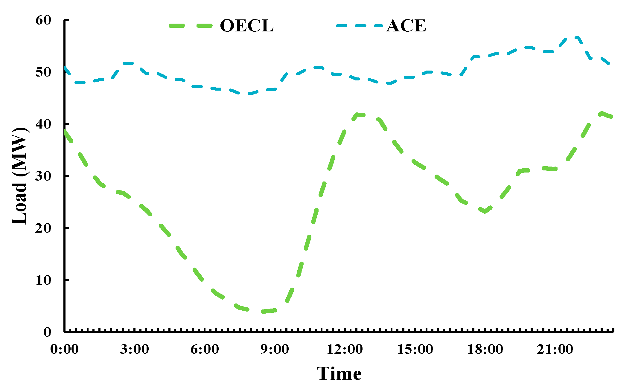
• The ACE and the OECL of a distribution system are comprehensively presented so as to consider the EV accommodation and charging load distribution holistically. Furthermore, EVs are divided into four major categories to discuss the corresponding OECL in detail.
• The proposed co-optimization model considers both the optimal dispatch of flexible resources and the optimal charging scheme for EVs with respect to security constraints, such as power balance, voltage limits and N − 1 security criterion.
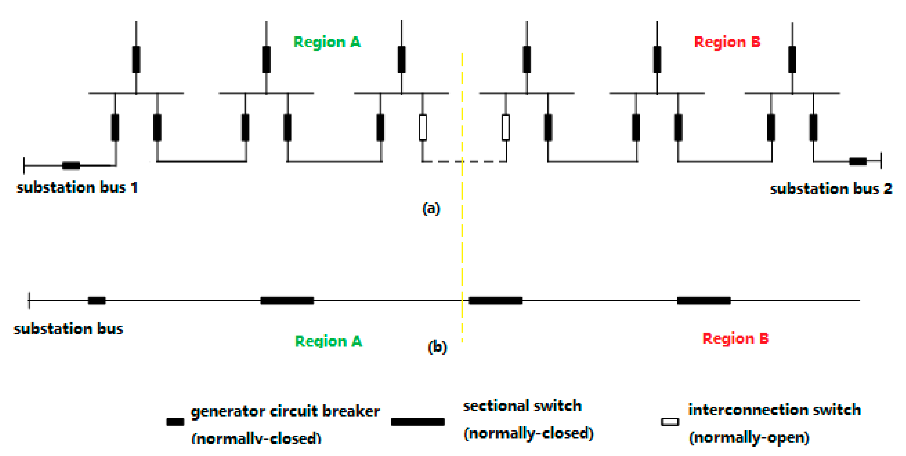
• A data-driven method is proposed to model EV charging behaviors, which is important in coordinating charging schedule. The distribution system is divided into multiple subareas according to its load characteristics. Coordinated charging optimization is performed in each subarea to meet its reliability standard while addressing its load characteristics.

The remainder of this paper is organized as follows. The framework of the model is illustrated in Section 2. The ACE evaluation model and the coordinated charging model are proposed in Section 3. Case studies are given to demonstrate the proposed method and to examine the impact of different factors in Section 4. Finally, conclusions and future research are presented in Section 5.

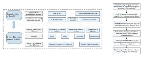
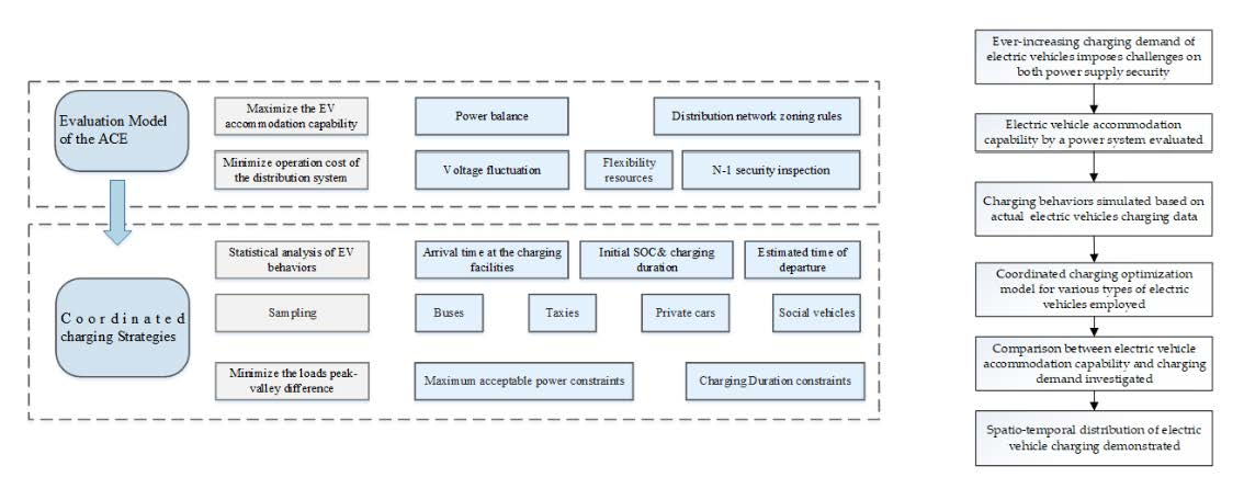
2. Framework of the Model

Different types of EV propulsion technology like pure EVs and PHEVs/EREVs are available, and the design of various DC-DC converter topologies for Battery Electric Vehicles (BEVs) and Plug-in Hybrid Electric Vehicles (PHEVs) are reviewed in Reference [21]. An overall picture of the current EV technology and prospects of future development are provided in Reference [22]. According to the different technical standards of the charging piles employed at present, EV charging modes are broadly divided into a quick mode (e.g., DC charging mode) and slow mode (e.g., constant AC power charging mode). Specifically, rapid DC charging applies to electric buses, cars, taxies and trucks, while slow constant power charging is targeted for small-scale EVs which obtain charging service mostly in public parking lots, large shopping centers, community garages, and household charging piles.

On this basis, an ACE evaluation model, with respect to power supply security constraints of the distribution system penetrated with flexible resources, is established at first. A coordinated EV charging optimization method is then proposed, taking into account the uncertainties in EV charging behaviors. EV charging load patterns are optimized according to real-life EV charging rules and EV ownership, and thereby a comparison between the OECL and the ACE evaluation is conducted. A schematic diagram of the model framework is shown in Figure 1.

3. Formulation of the Proposed Model

In this section, we first give some reasonable assumptions:

• All the charging loads of EVs at the charging stations or charging facilities that are connected to one bus are grouped into one load, and the ACE for each bus is evaluated in our model.
• EVs are divided into the following four categories in this paper: Electric buses, taxies, private cars, and social vehicles (mainly referring to rental cars). Each type of vehicle is affiliated with a corresponding charging rate.
• It is assumed that slow charging piles can interact with distribution system operators in real-time and the operators are capable of controlling the charging power and the duration for each EV once it is plugged into the system.

3.1. Evaluation Model of the ACE in a Distribution System

In order to maintain a secure and economic operation of the distribution system and accommodate as many EVs as possible, the objective function is to simultaneously maximize the EV accommodation capability and minimize operation cost of the distribution system with respect to the economic operational constraints.

(1) The objective function

The first objective of the model is to maximize the ACE, while the second objective is to minimize the operational costs of the distribution system which include the power purchase cost, the generation cost of DG units, the compensation for loads involved in the demand side response, and the ESS compensation cost. Then these two objective functions are normalized and integrated into one objective function based on the linear combination.

$$O_1^{\mathrm{bj}}={\displaystyle \sum _{t=1}^T{\displaystyle \sum _{i=1}^{N_{\mathrm{EV}}}{P}_{i,t}^{\mathrm{EV}}}}$$

(1)

$$O_2^{\mathrm{bj}}={\displaystyle \sum _{t=1}^T\left({\displaystyle \sum _{i=1}^{N_{\mathrm{node}}}{C}_t^{\mathrm{S}}{P}_{i,t}^{\mathrm{G}}}+{\displaystyle \sum _{g=1}^{N_{\mathrm{DG}}}{C}_{g,t}^{\mathrm{DG}}{P}_{g,t}^{\mathrm{DG}}+}{\displaystyle \sum _{d=1}^{N_{\mathrm{IL}}}{C}_t^{\mathrm{IL}}{P}_{d,t}^{\mathrm{IL}}}+{\displaystyle \sum _{r=1}^{N_{TL}}{C}_t^{\mathrm{TL}}\left|P_{r,t}^{TL}\right|}+{\displaystyle \sum _{m=1}^{N_{\mathrm{ESS}}}\left(C_t^{\mathrm{ESS}}\left|{\alpha }_{m,t}^{\mathrm{d}}{P}_{m,t}^{\mathrm{ESSD}}-{\alpha }_{m,t}^{\mathrm{c}}{P}_{m,t}^{\mathrm{ESSC}}\right|\right)}\right)}$$

(2)

$$O_{\mathrm{all}}^{\mathrm{bj}}={\omega }_1{O}_1^{\mathrm{bj}}-{\omega }_2{O}_2^{\mathrm{bj}}$$

(3)

where $O_1^{\mathrm{bj}}$, $O_2^{\mathrm{bj}}$, and $O_{\mathrm{all}}^{\mathrm{bj}}$ are respectively the ACE, the operational costs and the aggregative objectives of the model; T is the number of time periods in a day-ahead dispatch scheme; $P_{i,t}^{\mathrm{EV}}$ is the EV charging power at node i in time period t; N_EV is the number of nodes with EV charging facilities in the system; N_node, N_DG, N_IL, N_TL, and N_ESS are the numbers of nodes, DG units, interruptible loads, transferable loads, and the energy storage devices in the distribution system, respectively; $C_t^{\mathrm{S}}$, $C_{g,t}^{\mathrm{DG}}$, $C_t^{\mathrm{IL}}$, $C_t^{\mathrm{TL}}$, and $C_t^{\mathrm{ESS}}$ are the electricity purchasing price from the upstream transmission system, the unit generation cost of DG unit g, the unit compensation price for interruptible loads, the unit compensation price for transferable loads, and the unit compensation cost of the energy storage device in time period t, respectively; $P_{i,t}^{\mathrm{G}}$ is the active power injected at node i in time period t, and if node i is the slack bus then the pertinent active power is injected by the upstream supply transformer, otherwise the injected active power at node i is set as 0; $P_{g,t}^{\mathrm{DG}}$ is the actual output power of DG unit g (a wind turbine unit or photovoltaic unit) in time period t; $P_{d,t}^{\mathrm{IL}}$ is the active power curtailment of interruptible load d in time period t; $P_{r,t}^{\mathrm{TL}}$ is the transferred active power of transferable load r in time period t; $P_{m,t}^{\mathrm{ESSC}}$ and $P_{m,t}^{\mathrm{ESSD}}$ represents the active charging and discharging power of energy storage device m in time period t, respectively; ${\alpha }_{m,t}^{\mathrm{c}}$ and ${\alpha }_{m,t}^{\mathrm{d}}$ respectively represent the charging and discharging states of energy storage device m in time period t, and both are binary variables subject to ${\alpha }_{m,t}^{\mathrm{c}}$ + ${\alpha }_{m,t}^{\mathrm{d}}$ ≤ 1; and w₁, w₂ > 0 are the weights of the linear combination of the two normalized objective functions.

(2) Constraints

(a) Power balance constraints

The piecewise linearized DistFlow equations [19,23] are adopted in this paper to describe nodal power balances.

$$\begin{array}{l}\{\begin{array}{l}{P}_{i,t}^{\mathrm{G}}+P_{i,t}^{\mathrm{DG}}+{\alpha }_{i,t}^{\mathrm{d}}{P}_{i,t}^{\mathrm{ESSD}}=P_{\hspace{0.17em}i,t}^{\mathrm{D}}+P_{i,t}^{\mathrm{EV}}+P_{i,t}^{TL}-P_{i,t}^{IL}+{\alpha }_{i,t}^{\mathrm{c}}{P}_{i,t}^{\mathrm{ESSC}}+{\displaystyle \sum _{j\in {\Omega }_i}{\lambda }_{ij,t}^{}{P}_{ij,t}}+{\displaystyle \sum _{j\in {\Omega }_i}{\lambda }_{ij,t}^{}{r}_{ij}\frac{P_{ij,t}^{\mathrm{QU}}+Q_{ij,t}^{\mathrm{QU}}}{V_0^2}}\\ Q_{i,t}^{\mathrm{G}}=Q_{\hspace{0.17em}i,t}^{\mathrm{D}}+{\displaystyle \sum _{j\in {\Omega }_i}{\lambda }_{ij,t}^{}{Q}_{ij,t}}+{\displaystyle \sum _{j\in {\Omega }_i}{\lambda }_{ij,t}^{}{x}_{ij}\frac{P_{ij,t}^{\mathrm{QU}}+Q_{ij,t}^{\mathrm{QU}}}{V_0^2}}\end{array}\hspace{0.17em}\\ \hspace{0.17em}\forall i\in {\Omega }_{\mathrm{E}} \forall (ij)\in {\Omega }_{\mathrm{L}} \end{array}$$

(4)

where Ω_E and Ω_L represent the sets of nodes and branches in the distribution system, respectively; Ω_i is the set of nodes directly connected to node i; $P_{i,t}^{\mathrm{D}}$ and $Q_{i,t}^{\mathrm{D}}$ are the active and reactive load power at node i in time period t; $Q_{i,t}^{\mathrm{G}}$ is the reactive power injected at node i in time period t; P_ij,t and Q_ij,t are respectively the active and reactive power on branch ij in time period t; $P_{ij,t}^{\mathrm{QU}}$ and $Q_{ij,t}^{\mathrm{QU}}$ are used to estimate the quadratic terms of P_ij,t and Q_ij,t, and both can be approximated using the piecewise linearization approximation (PLA) method [19]; r_ij and x_ij are respectively the resistance and reactance of branch ij; and V₀ is the voltage amplitude at the slack bus. The network topology will change if an N − 1 contingency occurs—and, consequently, the power balance constraints will change accordingly. The state variable λ_ij,t is then introduced to represent the working state of branch ij in time period t; λ_ij,t = 0 or 1 stands for that branch ij is out of operation or in operation.

(b) Branch and node voltage constraints

$$\left|V_{j,t}-V_{i,t}-\frac{r_{ij}{P}_{ij,t}^{}+x_{ij}{Q}_{ij,t}^{}}{V_0}+\left(r_{ij}^2+x_{ij}^2\right)\frac{P_{ij,t}^{\mathrm{QU}}+Q_{ij,t}^{\mathrm{QU}}}{2V_0^3}\right| \le M(1-{\lambda }_{ij,t}^{})\forall i\in {\Omega }_{\mathrm{E}} \forall (ij)\in {\Omega }_{\mathrm{L}}$$

(5)

$$V_{j,t}=V^{\mathrm{G}},j\in {\Omega }_{\mathrm{S}}$$

(6)

$$V_i^{\min }\le V_{i,t}\le V_i^{\max }$$

(7)

where V_i,t is the voltage amplitude at node i in time period t; Ω_S represents the sets of the supply substation nodes; $V^{\mathrm{G}}$ is defined as the voltage of the supply substation; $V_i^{\max }$ and $V_i^{\min }$ are respectively the upper and lower limits of the voltage amplitude at node i; M is a very large positive number.

When λ_ij,t = 0, i.e., branch ij is out of operation, Equation (5) will never be binding, since M is very large; in other words, this constraint will always be met. When λ_ij,t = 1, i.e., branch ij is in operation, the left-hand side of the inequality in Equation (5) must be zero, indicating that the voltage drop constraint for branch ij is linearized.

(c) Power supply margin constraints

The N − 1 security inspection is widely used in power system planning for reliability testing, which requires that the system not only effectively supplies the load in the normal operation, but also can guarantee the load supply in case of failure of any single component connected in the system. Besides, feeder or unit contingencies will affect the power supply of the power system, which in turn affects the ACE of the distribution system.

According to the differences of the power backup condition and the power supply reliability level in the wiring mode, N − 1 security inspection is carried out based on the corresponding wiring mode. The changes of feeder connection in case of N − 1 contingencies are illustrated with two specific wiring examples.

For a line which is connected to two or more power sources at the same time and has the ability to transfer power, as shown in Figure 2a, when N − 1 contingencies occur in region B, the connection at the interconnection switch will be reconnected and the residual loads of region B, originally brought by Substation 2, will be transferred to Substation 1 [24,25]. Then, the load rate of Substation 1 is increased, which limits the ACE of nodes in this region. In this case, the power supply margin constraints, when N − 1 contingencies occur, can be summarized as constraints (8):

$${\displaystyle \sum _{i\in {\Omega }_{\mathrm{J}}}^{}{P}_i^{\mathrm{EV}}\le {\displaystyle \sum _{ij\in {\Omega }_{\mathrm{F}}}^{}{\lambda }_{ij}{P}_{ij}^{\mathrm{LCM}}}}-{\displaystyle \sum _{i\in {\Omega }_{\mathrm{A}}}^{}{P}_i^{\mathrm{D}}}-{\displaystyle \sum _{i\in {\Omega }_{\mathrm{B}}}^{}{P}_i^{\mathrm{D}}}$$

(8)

where Ω_J and Ω_F respectively represent the sets of nodes and feeders in wiring group l; and Ω_A and Ω_B are respectively the sets of nodes in regions A and B.

However, for a radial connection or multi-segment wiring type, like the single-end power supply line shown in Figure 2b, when N − 1 contingencies occur to a certain section of region B, the line in this area will lose power supply and all the loads connected will be cut off. In this situation, constraints (8) can be transformed into Equation (9).

$${\displaystyle \sum _{i\in {\Omega }_J}^{}{P}_i^{\mathrm{EV}}\le {\displaystyle \sum _{ij\in {\Omega }_s}^{}{\lambda }_{ij}{P}_{ij}^{\mathrm{LCM}}}}-{\displaystyle \sum _{i\in {\Omega }_{\mathrm{A}}}^{}{P}_i^{\mathrm{D}}}$$

(9)

(d) Nodal charging power constraints

$$0\le P_{i,t}^{\mathrm{EV}}\le P_i^{\mathrm{SME}}$$

(10)

where $P_i^{\mathrm{SME}}$ is the sum of the rated charging power of all charging piles connected to node i.

(e) Transformer capacity constraints

The active and reactive power constraints of a power supply transformer are as follows:

$$\left|P_{k,t}^{\mathrm{G}}\right|\le P_k^{\mathrm{Gmax}}$$

(11)

$$\left|Q_{k,t}^{\mathrm{G}}\right|\le Q_k^{\mathrm{Gmax}}$$

(12)

where $P_k^{\mathrm{Gmax}}$ and $Q_k^{\mathrm{Gmax}}$ are respectively the upper limits of the active and reactive power of the transformer k.

(f) Feeder capacity constraints

$$\left|P_{ij,t}\right|\le P_{ij}^{\mathrm{LCM}} \forall (ij)\in {\Omega }_L$$

(13)

where P_ij,t is the active power of feeder ij in time period t; $P_{ij}^{\mathrm{LCM}}$ is the active power capacity limit of feeder ij.

(g) DG output constraints

$$0<P_{w,t}^{\mathrm{wind}}<P_w^{\max }$$

(14)

$$0<P_{p,t}^{\mathrm{pv}}<P_p^{\max }$$

(15)

where $P_w^{\max }$ and $P_{w,t}^{\mathrm{wind}}$ are, respectively, the capacity and actual active power output of wind turbine w in time period t; $P_p^{\max }$ and $P_{p,t}^{\mathrm{pv}}$ are, respectively, the capacity and the actual active power output of PV unit p in time period t.

(h) DR constraints

In this paper, the interruptible loads (ILs) and the transferable loads (TLs) are employed to implement DR. The parameters associated with the ILs include the duration and quantity of the interruptible loads and the summation of the TLs are kept constant within one scheduling period.

$${\displaystyle \sum _{d=1}^{N_{\mathrm{IL}}}{P}_{d,t}^{\mathrm{IL}}}\le {\delta }_t^{\mathrm{IL}}{\displaystyle \sum _{i=1}^{N_{\mathrm{node}}}{P}_{i,t}^{\mathrm{D}}}$$

(16)

$${\displaystyle \sum _{r=1}^{N_{\mathrm{TL}}}\left|P_{r,t}^{\mathrm{TL}}\right|}\le {\delta }_t^{\mathrm{TL}}{\displaystyle \sum _{i=1}^{N_{\mathrm{node}}}{P}_{i,t}^{\mathrm{D}}}$$

(17)

$$T_d^{\min }\le T_d\le T_d^{\max }$$

(18)

$${\displaystyle \sum _{t=1}^T{\displaystyle \sum _{r=1}^{N_{\mathrm{TL}}}{P}_{r,t}^{\mathrm{TL}}}=0}$$

(19)

where ${\delta }_t^{\mathrm{IL}}$ and ${\delta }_t^{\mathrm{TL}}$ are respectively the maximum allowed proportion of the ILs and the TLs over the total loads in time period t; T_d, $T_d^{\max }$ and $T_d^{\min }$ are respectively the load interruption time, and the allowed upper and lower limits of the interruption time period of interruptible load d.

(i) State constraints for energy storage devices

The calculation method of the charged state of the ESS is shown in Equations (20) and (21), which impose the upper and lower limits of the charged state of the energy storage devices.

$$S_m=\frac{\left|{\alpha }_m^{\mathrm{d}}{P}_{m,t}^{\mathrm{ESSD}}-{\alpha }_m^{\mathrm{c}}{P}_{m,t}^{\mathrm{ESSC}}\right|}{P_m^{\max }}$$

(20)

$$S_m^{\min }\le S_m\le S_m^{\max }$$

(21)

where S_m is the charged state of the energy storage device m; $P_m^{\max }$ is the capacity of the energy storage device m; $S_m^{\max }$ and $S_m^{\min }$ are the upper and lower limits of the charged state of device m, respectively.

3.2. The Coordinated Charging Optimization Model

Based on available data of public charging piles and special charging stations for EVs, in a Chinese coastal province, electric buses, taxies, and social vehicles usually prefer quick charging, and terminate charging after an expected level of the state of charge (SOC) is attained. Therefore, these kinds of EVs are not suitable for participating in charging scheduling optimization. Private EV cars usually adopt slow charging at office locations or at home. Parking time of private EV cars at charging piles is normally long, and is then suitable for participation in the coordinated charging optimization. Parameters of different types of EVs discussed in this paper are listed in

Table 1. Parameters of different types of electric vehicles.

Vehicle Type	Battery Size (kWh)	Charging Rate (kW)	Type of Charger
Bus	324	80	DC
Taxi	57	40	DC
Social vehicle	57	40	DC
Car	25.6	7	AC

.

Specific implementation methods of the coordinated charging optimization model include the following steps: (1) EV ownership and charging rules are statistically obtained, and a probability model of charging behaviors is attained; (2) the well-established Monte Carlo simulation is used to generate the charging behavior parameters; (3) the coordinated charging optimization is finally obtained based on sampling results.

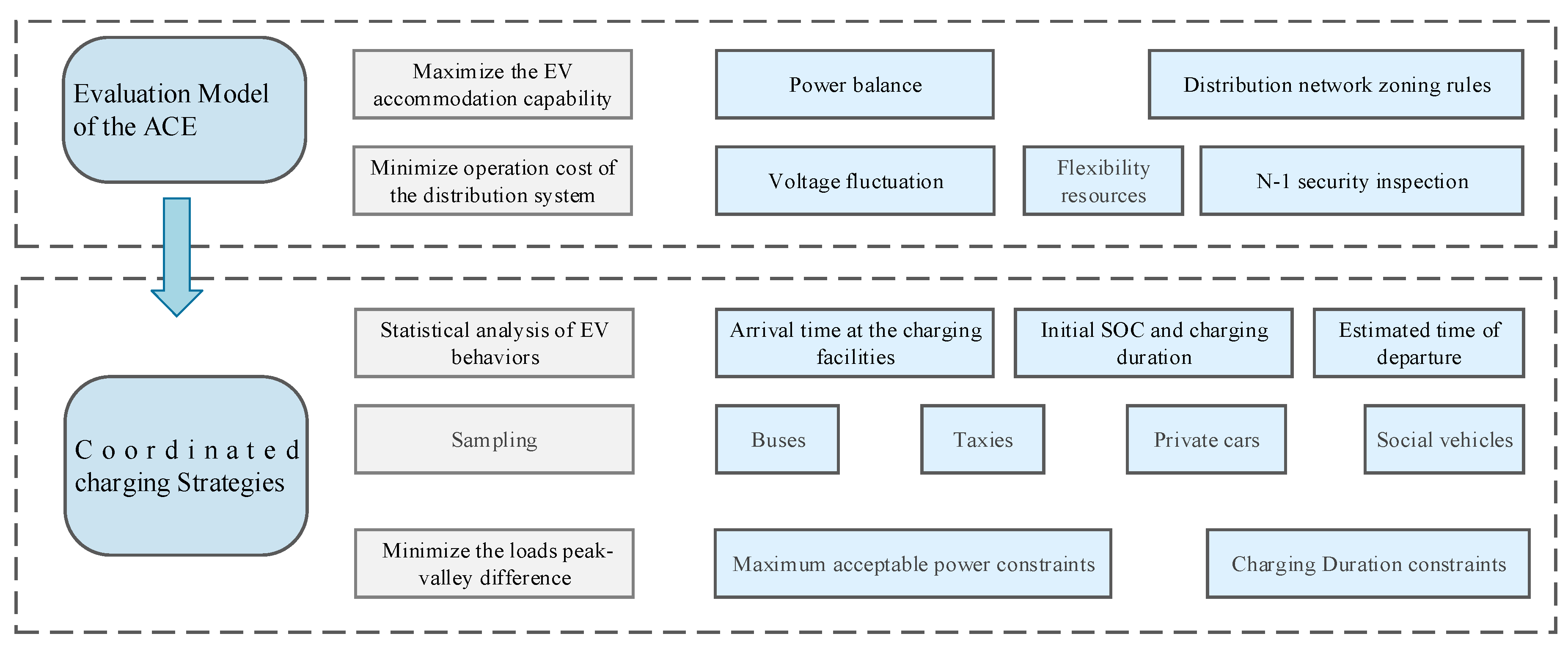
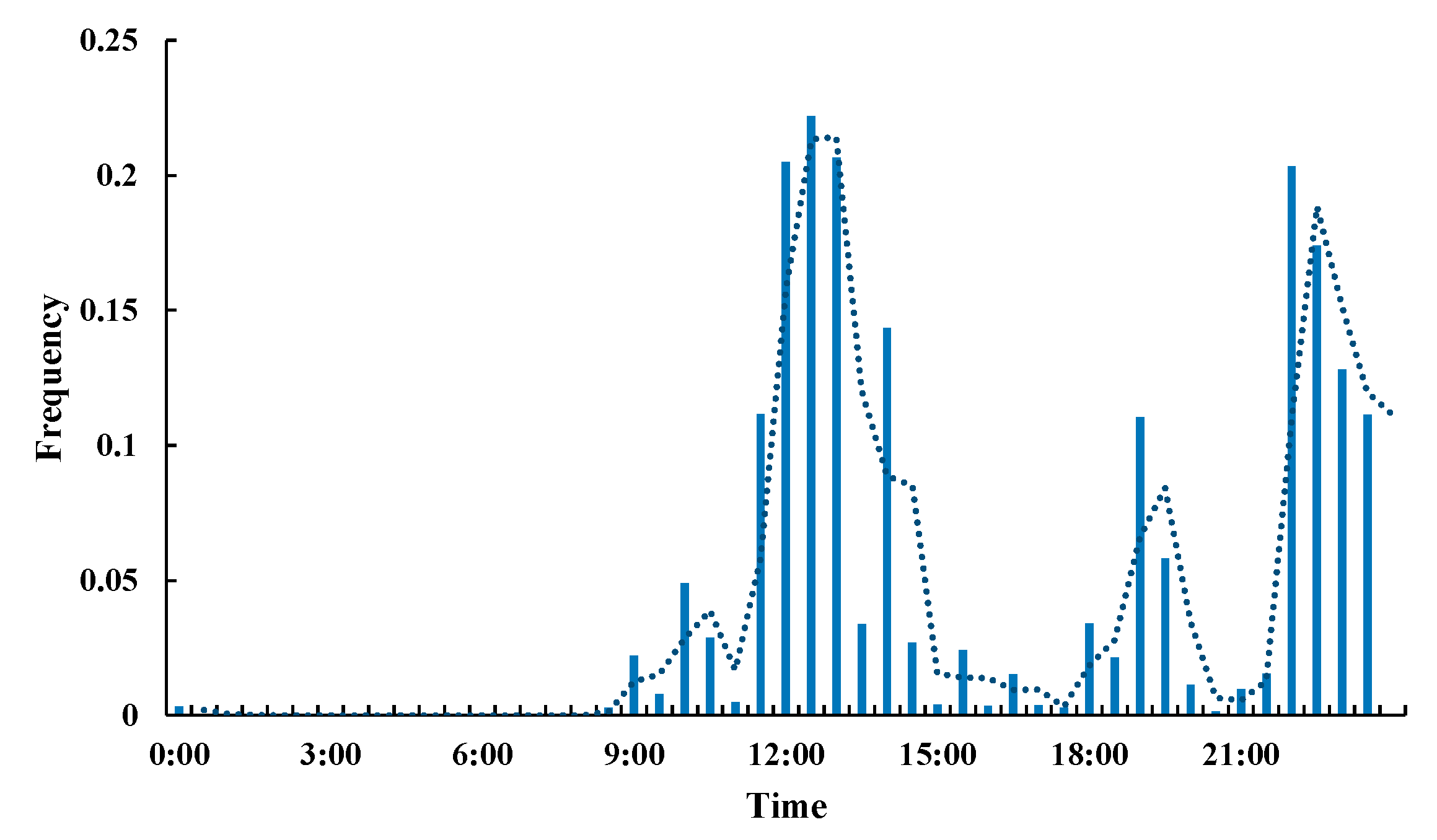
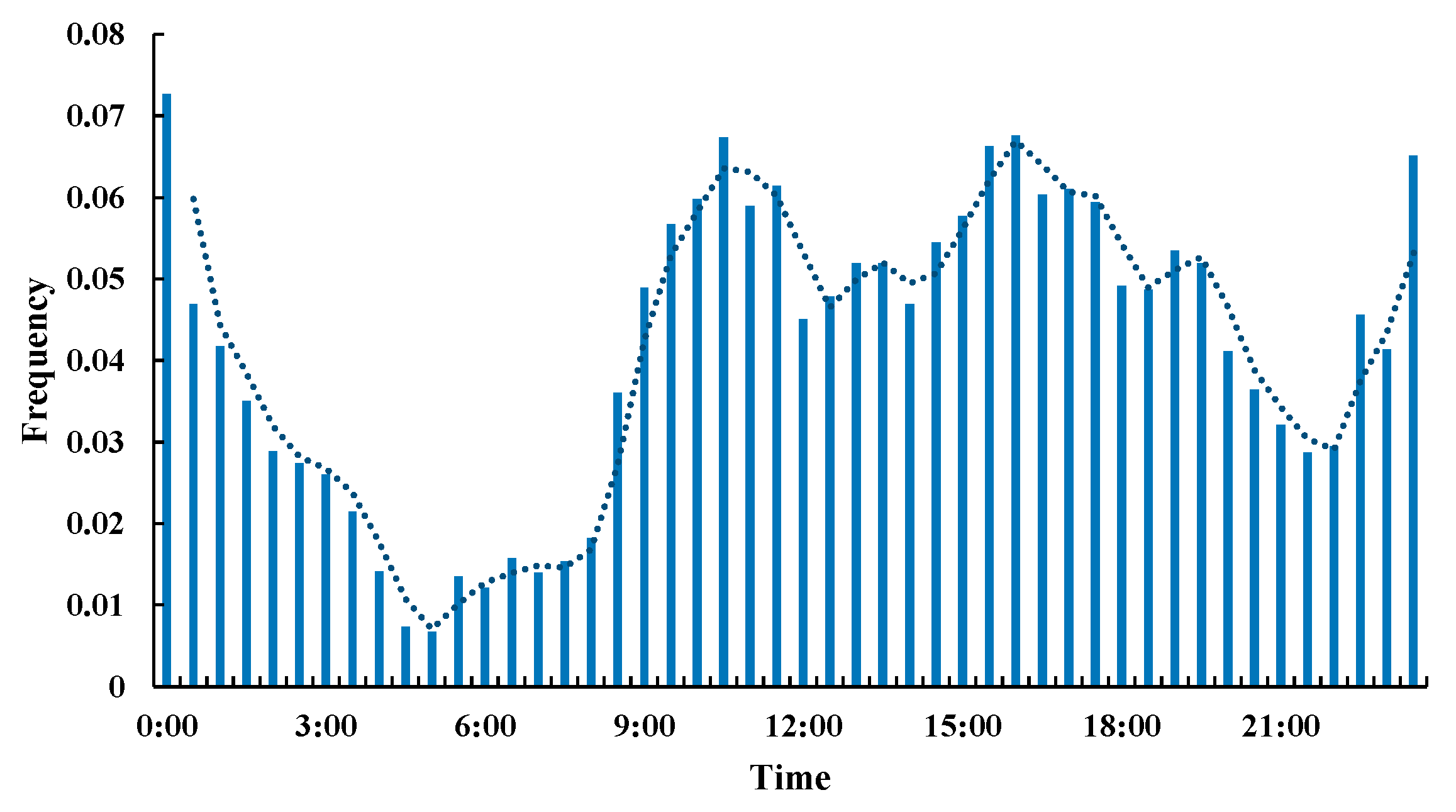
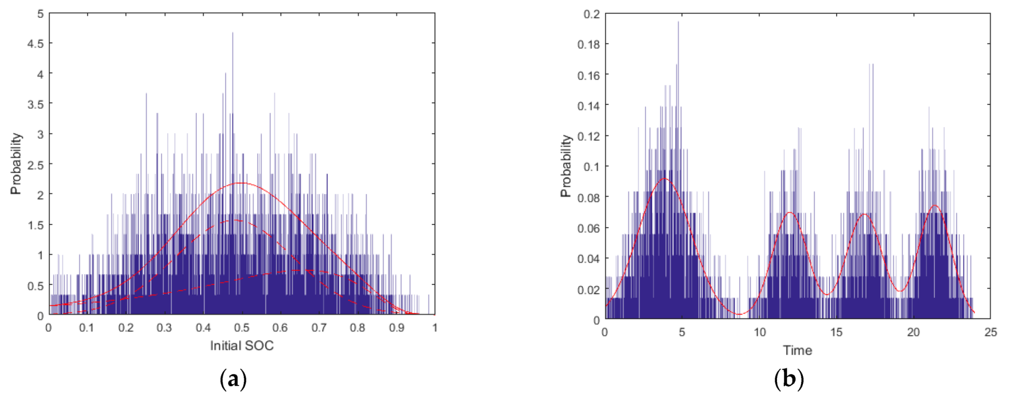
3.2.1. Statistical Analysis

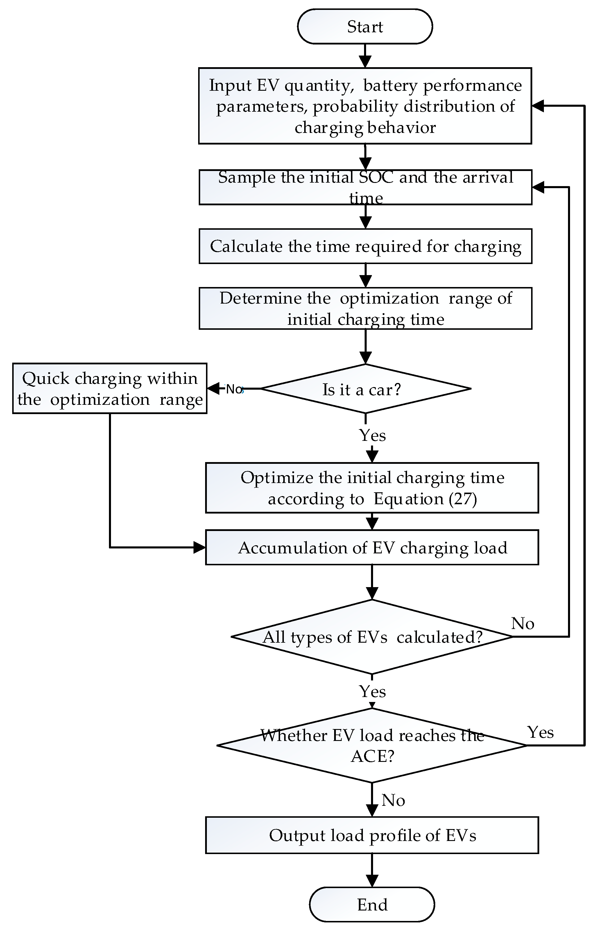
Based on the statistical analysis of EV charging data, transportation rules of electric buses, taxies, social vehicles, and private cars are obtained by piecewise fitting using standard fitting methods. Figure 3 and Figure 4 show the sample distributions of the initial charging time of EVs for buses and social vehicles. The probability distributions of the charging durations for four types of EVs are approximated in Equations (22)–(26).

From the analysis of EV charging data, the charging duration of buses approximately follows a lognormal distribution, and its probability density function can be expressed as in Equation (22).

$$f_s^{\mathrm{bus}}(t_{}^{\mathrm{bin}})=A^{\mathrm{bus}}\frac{1}{t_{}^{\mathrm{bin}}{\sigma }_{}^{\mathrm{bus}}\sqrt{2\pi }}\exp \left(-\frac{{(\ln t_{}^{\mathrm{bin}}-{\mu }_{}^{\mathrm{bus}})}^2}{2{\left({\sigma }_{}^{\mathrm{bus}}\right)}^2}\right)$$

(22)

where $f_s^{\mathrm{bus}}$ is the probability distribution function of the charging duration of buses; t^bin is the charging duration of a bus; A^bus is the function amplitude; μ^bus and σ^bus are respectively the mean and the standard deviation of the logarithmic charging duration.

The probability density function of the initial SOC of electric taxies is divided into two stages based on their charging start time; each approximately follows a lognormal distribution, as shown in Equations (23) and (24). Based on the distributions of the initial SOC, the charging duration can be estimated as in Equation (25). The probability distribution function of the initial SOC for private cars is consistent with Equation (24), due to similar transportation patterns.

$$f_1^{\mathrm{taxi}}(S_{}^{\mathrm{tin}})=A_1^{\mathrm{taxi}}\frac{1}{{\sigma }_1^{\mathrm{taxi}}\sqrt{2\pi }}\exp \left(-\frac{{\left[\ln (R(1-S_{}^{\mathrm{tin}}))-{\mu }_1^{\mathrm{taxi}}\right]}^2}{2{\left({\sigma }_1^{\mathrm{taxi}}\right)}^2}\right),0\le t\le 14$$

(23)

$$f_2^{\mathrm{taxi}}(S_{}^{\mathrm{tin}})=A_2^{\mathrm{taxi}}\frac{1}{R(1-S_{}^{\mathrm{tin}}){\sigma }_2^{\mathrm{taxi}}\sqrt{2\pi }}\exp \left(-\frac{{\left[\ln (R(1-S_{}^{\mathrm{tin}}))-{\mu }_2^{\mathrm{taxi}}\right]}^2}{2{\left({\sigma }_2^{\mathrm{taxi}}\right)}^2}\right),14<t\le 24$$

(24)

$$t^{\mathrm{tin}}=\frac{P_{\mathrm{bat}}^{\mathrm{taxi}}}{P_{\mathrm{ch}}^{\mathrm{taxi}}}\left(S^{\exp }-S^{\mathrm{tin}}\right)$$

(25)

where $f_1^{\mathrm{taxi}}$ and $f_2^{\mathrm{taxi}}$ are the piecewise probability distribution function of the initial SOC of taxies at different times; $A_1^{\mathrm{taxi}}$ and $A_2^{\mathrm{taxi}}$ are the function amplitude; S^tin and S^exp are respectively the initial SOC and the expected SOC of the taxi; t^tin is the charging duration of a taxi; R stands for taxi endurance; ${\mu }_1^{\mathrm{taxi}}$, ${\mu }_2^{\mathrm{taxi}}$ and ${\sigma }_1^{\mathrm{taxi}}$, ${\sigma }_2^{\mathrm{taxi}}$ are respectively the mean and the standard deviation of the driving distance at different times; $P_{\mathrm{ch}}^{\mathrm{taxi}}$ and $P_{\mathrm{bat}}^{\mathrm{taxi}}$ are respectively the charging rate and the battery capacity of taxies.

Charging rules of social vehicles are analyzed using data from public charging stations, as most social vehicles get access to charging services at public charging stations. The statistics show that the charging duration approximately follows a normal distribution shown in Equation (26).

$$f_s^{\mathrm{social}}(t_{}^{\sin })=A^{\mathrm{social}}\frac{1}{{\sigma }_{}^{\mathrm{social}}\sqrt{2\pi }}\exp \left(-\frac{{(t_{}^{\sin }-{\mu }_{}^{\mathrm{social}})}^2}{2{\left({\sigma }_{}^{\mathrm{social}}\right)}^2}\right)$$

(26)

where $f_s^{\mathrm{social}}$ is the probability distribution function of the charging duration of social vehicles; A^social is the function amplitude; t^sin is the charging duration of a social vehicle; μ^social and σ^social are respectively the mean and the standard deviation of the charging duration.

Combining transportation and charging data for different types of EVs, MATLAB’s fitting toolbox is used to fit the probability distribution parameters. The statistical analysis of other charging behavior parameters can also be adopted in the same way.

3.2.2. Sampling

Monte Carlo simulation is used to sample the initial SOC, the charging duration, and the arrival time of EVs, with input data of EV ownership, performance parameters, and a probability distribution of charging behavior parameters. The sampling results of the initial SOC and arrival time of taxies are shown in Figure 5 as an example.

3.2.3. Coordinated Charging Optimization

The objective function of the coordinated charging optimization model is to minimize the load’s peak-valley difference within the system scheduling period.

$$\min P^{\mathrm{cut}}=P^{\mathrm{peak}}-P^{\mathrm{valley}}$$

(27)

where P^cut is the peak-valley difference of the system load; P^peak and P^valley are the load peak and valley during the system scheduling period, respectively.

The charging power of electric buses, taxies, and social vehicles are respectively formulated in Equations (28)–(30) based on sampling results.

$$P_{i,t}^{\mathrm{bus}}={\displaystyle \sum _{v=1}^{N_i^{\mathrm{bus}}}{P}_{\mathrm{ch}}^{\mathrm{bus}}\times b_{v,t}^{\mathrm{bus}}}$$

(28)

$$P_{i,t}^{\mathrm{taxi}}={\displaystyle \sum _{v=1}^{N_i^{\mathrm{taxi}}}{P}_{\mathrm{ch}}^{\mathrm{taxi}}\times b_{v,t}^{\mathrm{taxi}}}$$

(29)

$$P_{i,t}^{\mathrm{social}}={\displaystyle \sum _{v=1}^{N_i^{\mathrm{social}}}{P}_{\mathrm{ch}}^{\mathrm{social}}\times b_{v,t}^{\mathrm{social}}}$$

(30)

where $P_{i,t}^{\mathrm{bus}}$, $P_{i,t}^{\mathrm{taxi}}$, and $P_{i,t}^{\mathrm{social}}$ refer to the total charging power outputs of buses, taxies, and social vehicles connected to node i within time period t, respectively; $P_{\mathrm{ch}}^{\mathrm{bus}}$ and $P_{\mathrm{ch}}^{\mathrm{social}}$ are the charging rates of buses and social vehicles, respectively; $b_{v,t}^{\mathrm{bus}}$, $b_{v,t}^{\mathrm{taxi}}$, and $b_{v,t}^{\mathrm{social}}$ are respectively the charging states of the vth bus, taxi, and social vehicle in time period t with values of 1 or 0 standing for the charging and the idle condition, respectively; $N_i^{\mathrm{bus}}$, $N_i^{\mathrm{taxi}}$, and $N_i^{\mathrm{social}}$ are the numbers of buses, taxies, and social vehicles connected to node i for charge.

Equation (31) shows the initial charging time constraint of private cars, while (32) ensures that EVs be charged to the expected SOC before departure.

$$t_v^{\mathrm{arr}}\le t_v^{\mathrm{real}}\le t_v^{\mathrm{dep}}$$

(31)

$$t_v^{\mathrm{real}}+t_v^{\mathrm{last}}\le t_v^{\mathrm{dep}}$$

(32)

where $t_v^{\mathrm{arr}}$, $t_v^{\mathrm{real}}$, $t_v^{\mathrm{dep}}$, and $t_v^{\mathrm{last}}$ are respectively the times when the vth EV arrives at the charging pile, the optimized initial charging time of the vth EV, departure time of the vth EV, and the charging duration.

The charging power of private cars can be calculated by Equation (33). The OECL is then computed with the charging power of other EVs, which should not exceed the corresponding ACE.

$$P_{i,t}^{\mathrm{car}}={\displaystyle \sum _{v=1}^{N_i^{\mathrm{car}}}{P}_{\mathrm{ch}}^{\mathrm{car}}\times b_{v,t}^{\mathrm{car}}}$$

(33)

$$P_{i,t}^{\mathrm{REV}}=P_{i,t}^{\mathrm{bus}}+P_{i,t}^{\mathrm{taxi}}+P_{i,t}^{\mathrm{social}}+P_{i,t}^{\mathrm{car}}$$

(34)

$$P_{i,t}^{\mathrm{REV}}\le P_{i,t}^{\mathrm{EV}}$$

(35)

where $P_{i,t}^{\mathrm{car}}$ refers to the charging power of private cars connected to node i within time period t; $P_{\mathrm{ch}}^{\mathrm{car}}$ is the rated charging power of a private car; $b_{v,t}^{\mathrm{car}}$ is the charging state of the vth private car in time period t; $N_i^{\mathrm{car}}$ is the number of private cars connected to node i for charge; $P_{i,t}^{\mathrm{REV}}$ represents the OECL connected to node i within time period t.

The optimization procedure is shown in Figure 6.

3.3. Relationship between the Two Models

The accommodation capability for EVs, calculated by the ACE evaluation model, is transferred to the coordinated charging optimization problem through $P_{i,t}^{\mathrm{EV}}$. Then sampling for different types of EVs is conducted, and the OECL is obtained by the coordinated charging optimization model using the real-life EV charging and transportation rules. When there is a significant mismatch between the charging demand and the optimized charging power attained in the upper level, if the charging demand is lower than that in ACE it will be fully supplied—otherwise the charging demand will be partially supplied with the amount of the upper limit.

4. Case Studies

4.1. Solving Method

The ACE evaluation model is a mixed-integer linear programming problem. The YALMIP platform and solver CPLEX (the Simplex method implemented in the °C programming language) [26] are used to solve the problem. The Particle Swarm Optimization (PSO) algorithm [27,28] is then adopted to solve the coordinated charging optimization problem.

4.2. System Settings

In this section, an actual distribution system in a coastal area of China is employed to demonstrate the proposed method. There are seven 110 kV substations, 376 nodes, 368 branches, 6 PV units, and two wind farms, with 51 nodes connected to EV charging facilities in this system. The system is divided into eight power grid units according to the division rules mentioned in Section I. The numbers of EVs in different parts of the distribution system are listed in

Table 2. Numbers of electric vehicles in different parts of the distribution system.

Vehicle Type	Grid-1	Grid-2	Grid-3	Grid-4	Grid-5	Grid-6	Grid-7	Grid-8
Bus	52	35	13	10	6	12	19	25
Taxi	50	19	14	4	5	10	15	17
Social vehicle	429	204	117	53	48	92	136	165
Car	302	161	94	18	35	74	113	170

. The basic load profile of a typical day is selected to represent the system basic load. Based on wind speed and light intensity data in a certain time period, the forecasted outputs of the DGs can be obtained by employing the Latin hypercube sampling algorithm [29].

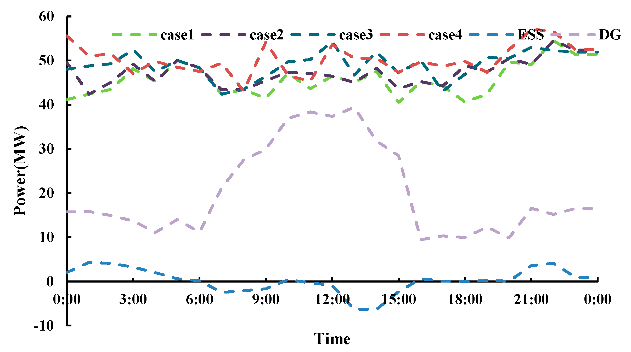
4.3. Comparisons of Results among Multiple Cases

In order to demonstrate the impact of flexible resources on the ACE, four different cases are investigated:

Case 1: The original system without flexible resources;

Case 2: An updated system with DG integration into the original system;

Case 3: Case 2 with ESS integrated;

Case 4: An integrated system with DG, ESS, and DR.

The accommodation capability for EVs by the distribution system under different cases and outputs from flexible resources are shown in Figure 7, where the positive value of energy storage represents the released energy, and the negative value represents the stored energy. By comparing the ACEs between Case 1 and Case 2 in Figure 7, it is clear that DG integration can effectively improve the ACE of the distribution system in the daytime as the majority of DG units are photovoltaic units that mainly generate electricity during the daytime. The accommodation level for the power output from DGs can also be enhanced in the low load period as EVs can be charged at night. In Case 3, the ESS stores the unconsumed energy of DGs during the valley load period, and releases it in the peak load period, so that the ACE is enhanced. Among the results of Cases 1-4, the ACE of the distribution system is the highest in Case 4, as the integration of multiple flexible resources increases the overall duration for accommodating EV loads, and hence enhances the ACE of the distribution system.

The comparison of the four cases shows the ACE promotion effects by the integration of flexible resources. However, the addition of flexible resources will not yield a particularly large increase in the ACE, as the ACE is also affected by the transmission capacity of the power distribution system. Under the condition that the power grid structure remains unchanged, the load-bearing capacity of the system is limited.

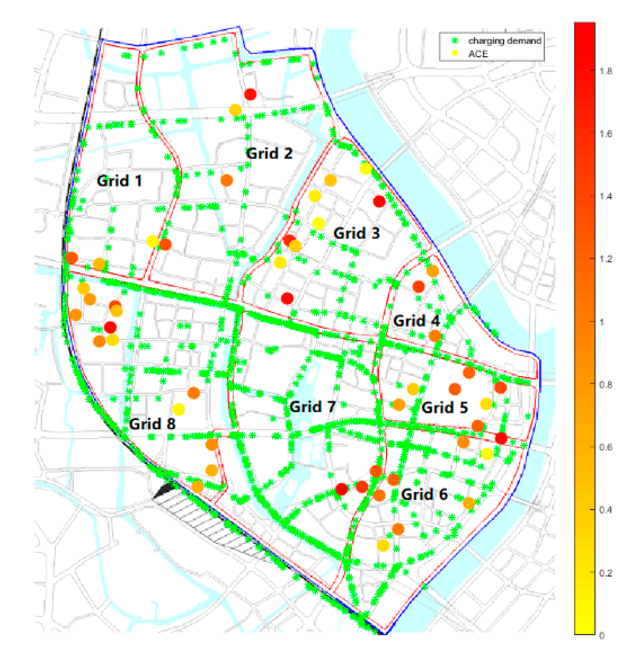
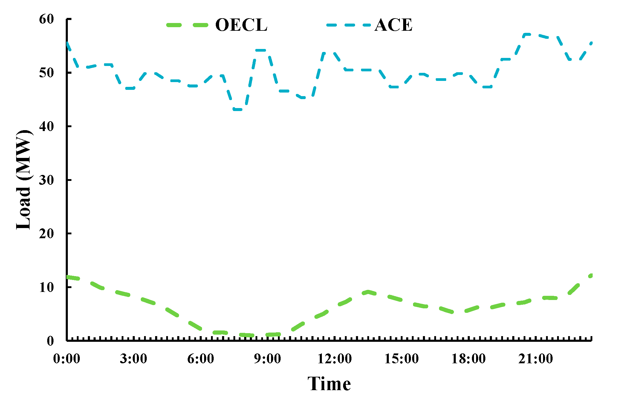
4.4. Spatiotemporal Distribution of the ACE

Figure 8 shows the daily system load profile and the ACE time variation curve. It can be seen that the ACE is variable with time, and the ACE is limited by the peak load of the system.

Figure 9 shows the spatial distribution of the ACE and charging demand in a typical time period. Please note that only the geographical locations of the nodes connected with EV charging facilities are shown in this figure, while the remaining nodes and feeders are not shown. The color of each circular node represents the strength degree of its ACE such that higher ACE values are represented by red nodes and lower ACE values are represented by yellow nodes. The density of green dots in the figure reflects the density of EV charging demands on the road, obtained by applying the multi-agent-based microscopic traffic assignment model [30]. As shown in Figure 9, there are some nodes in a grid, where the ACEs are adequate to satisfy the charging demands. However, there are still some cases where the ACEs do not match the charging demands. For example, in Grid-8, the ACEs at some nodes are sufficient, but the EV charging demands on the road around these nodes are relatively sparse, meaning that a part of the charging facilities would be idle. On the other hand, the charging demand in the central part of the region like Grid-7 is high, but the ACE nearby is relatively low. EV users have to get EVs charged at a relatively far distance, which may increase traffic congestion.

It should be mentioned that access to EVs is not limited to nodes with existing charging stations or scattered charging piles. All nodes in the distribution network are supposed to be able to accept EVs for charging, since the planning of new charging facilities is taken into account in this system. The results of the ACE of the whole distribution network at a typical time point in a day are shown in Figure 10. In this figure, each part of the distribution network is colored according to the ACE, with color strength proportional to the ACE.

Comparing Figure 9 and Figure 10, the difference between the ACE of nodes with charging facilities and the ACE of the system mainly lies in Grid-7. The ACE of nodes with charging facilities in Grid-7 is weak, while the overall ACE of the whole distribution system is the strongest among all parts of the system. This demonstrates that the distribution network structure corresponding to Grid-7 is relatively strong, which can accommodate the access of charging loads of a large number of EVs with secure operation maintained. However, due to the limited number of existing charging facilities and other reasons like city construction, the current ACE of Grid-7 is lower. Then Grid-7 is a good candidate region for new EV charging stations. The evaluation of the capability of the whole distribution network can explore its potential of accommodating EVs and provide some guidance for the subsequent charging facility planning.

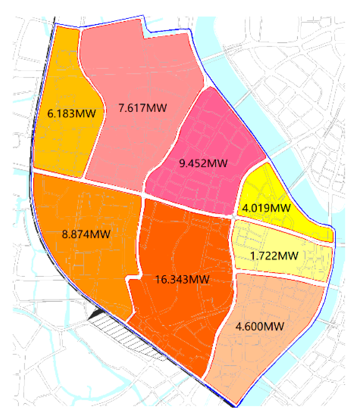
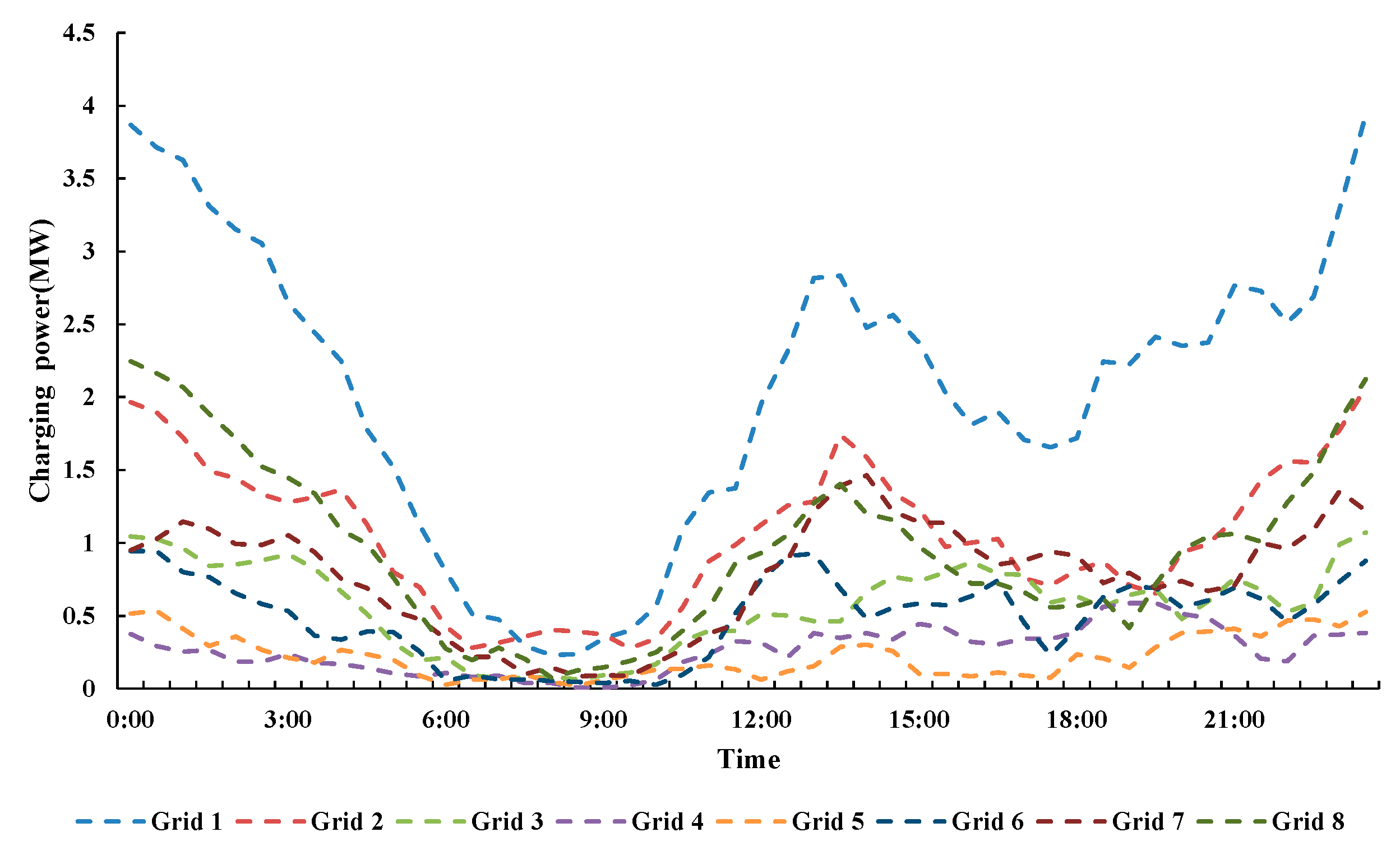
4.5. The Regional Distribution of OECL

EV ownership and EV types all correspond to the basic loads, and load types in the power grids, so it is necessary to explore the regional OECL distribution characteristics.

As shown in Figure 11, the load curve trough time of each subarea is identical and is around 08:00. In connection with a real-life situation, this period is generally the departure time of EVs. Besides, the OECL in Grid 1 is the largest among all the grids concerned because of the high EV ownership, and there are two load peaks around 13:00 and 22:00. This is because this subarea is mainly composed of residence and office areas, which reveals a behavior of getting out early and coming back at dusk. Therefore, there is a charging peak after EV owners go home at night; meanwhile, the charging of social vehicles and buses near the office area during the day forms another charging peak. The load structure of Grid 6 is consistent with that of Grid 1, so it presents a similar charging load profile. Grid 3 is the downtown area and charging loads mainly arrive during the day, while EV charging loads in Grid 4 mainly appear at night as this grid is dominated by residential areas. The charging load profile analyses for the rest of the grids are similar and will not be detailed.

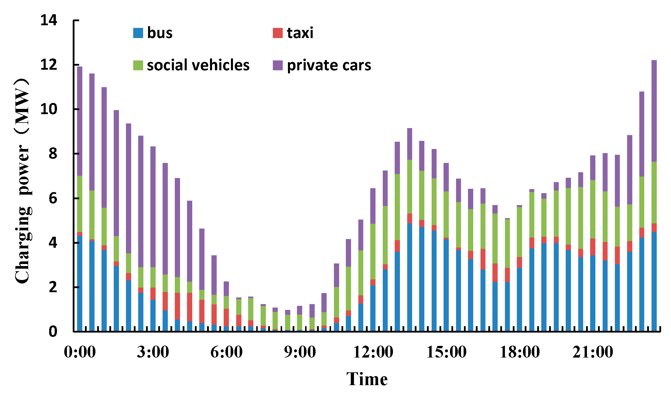
4.6. OECL for Different Types of EVs

The OECLs for different types of EVs are obtained and compared with the ACE to explore the impact of EV categories on the OECL.

As shown in Figure 12, electric buses have a significant impact on the EV charging load profile, due to their high charging power and quick charge mode. Taxies mainly charge at night after the evening rush hours on the basis of a shift system. The charging load of a private car is mostly distributed in the load trough stage under the coordinated charging optimization, which has a prominent effect of filling the load valley. However, the charging load distribution of social vehicles is more random, but mainly concentrated between 14:00 and 23:00.

In general, the charging load of EVs is high between 13:00–02:00 (next day) and low during 04:00–11:00, which is basically consistent with the system load profile. Therefore, it is necessary to cope with EV charging behaviors in the future.

Figure 13 shows the profile of the ACE and the OECL computed by the proposed model. It is obvious that the current distribution system has a wide capacity margin to accommodate EVs.

4.7. Accommodation Potential Analysis

With rapid developments of EVs and loads, the load accommodation capability of the distribution system will change accordingly, which will affect the ACE and its spatial and temporal distributions. Therefore, in order to test and verify the reliability of the current system, it is necessary to explore changes in the ACE and OECL, with respect to EV growth and load development. In this case, the current network structure and integration of flexible resources are kept unchanged, while the load level and EV ownership are projected to grow in the next five years. The results are shown in Figure 14.

Consider the average daily profile of the ACE and the OECL in Figure 14. Most of the time within a day, the distribution system maintains a certain ACE margin over the OECL. However, there are times that both the ACE and OECL are relatively close, especially around 14:00. This narrower ACE margin is a result of the projected future EV and load growth. On the supply side, this indicates that the system needs to be expanded to cope with the load growth over time. It is also important to provide guidance to manage different charging behaviors, especially the usage of quick charging that has a higher impact on the distribution system.

5. Conclusions

This paper explores the ACE and the OECL of a distribution system with high penetrations of flexible resources, such as DGs and ESSs. At the same time, the spatiotemporal distributions of the ACE are investigated. The EV accommodation potential of a distribution system is also explored from the perspective of load growth. The following conclusions are drawn:

(1)

The participation of multiple flexible resources can effectively improve the ACE. To be specific, the impacts of DGs, especially PVs, are mainly demonstrated in the midday load peak period, and the ACE can be increased up to 10% for the studied sample system.

(2)

By considering credible N − 1 contingencies and zoning rules in the distribution network, more accurate ACE can be attained.

(3)

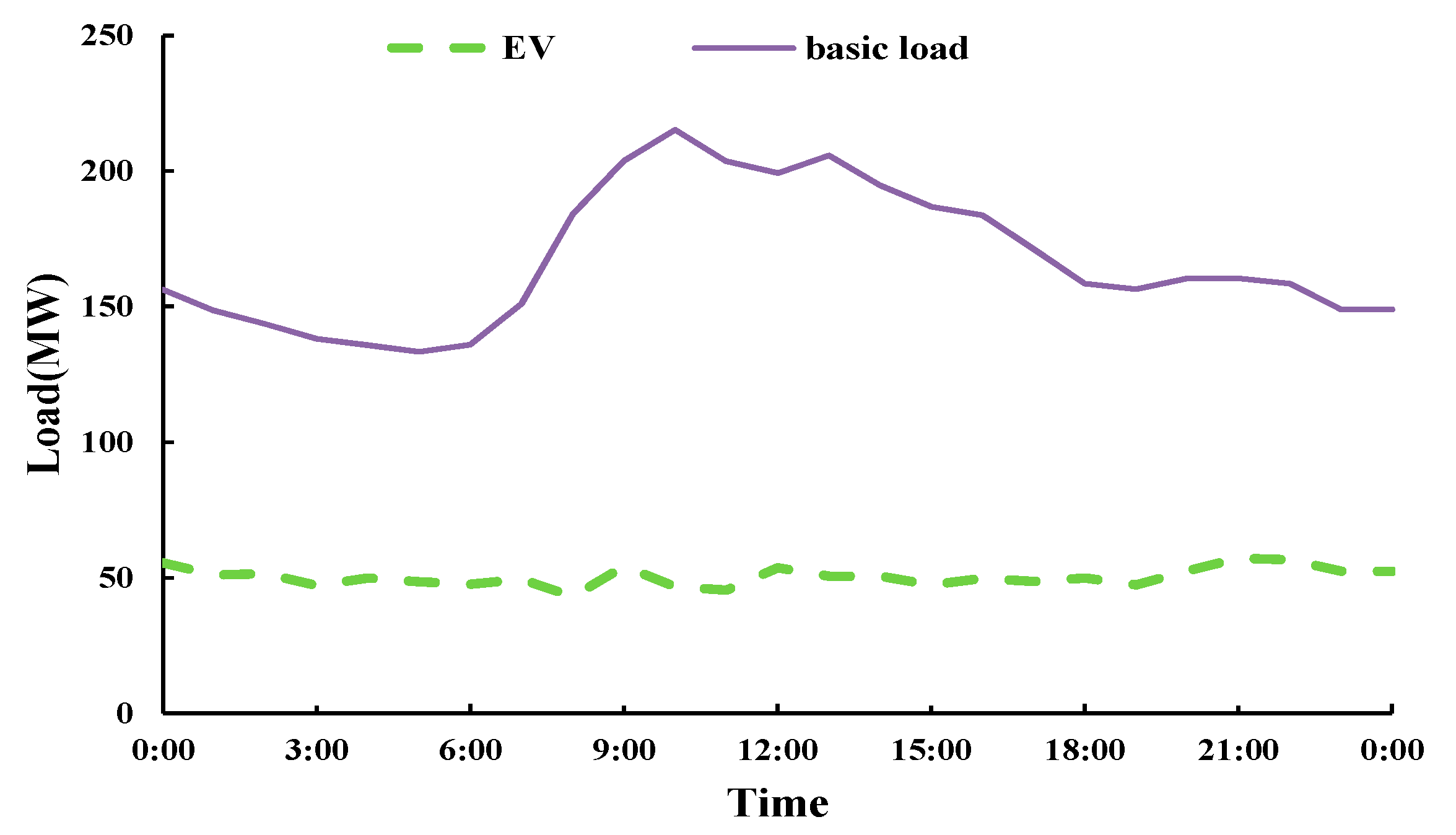
The regional OECL reflects the charging load distribution of EVs in different parts of the power distribution system, while the OECL evaluation for different types of EVs reveals the composition and temporal distribution of EV charging loads. The peak load of EVs occurs at around 14:00 and 23:00, while the amount and time-space distribution of the EV charging load are mainly determined by electric buses and private cars. Coordinated charging optimization of private cars can help mitigate the load peak-valley difference.

(4)

From the perspective of traffic flow or the coordinated charging strategies, there is a certain degree of spatial and temporal distribution mismatch between the ACE and EV charging. In this case, analysis results of the proposed model lay the foundation for distribution system expansion and the planning and construction of the EV charging facilities in the future.

Future work will address the impacts of the vehicle-to-grid (V2G) system on both EV charging behaviors and the distribution system. In addition, the extension of the current work to the ACE evaluation in a V2G environment will also be investigated in our future research efforts.

References

1. Sortomme, E.; Hindi, M.M.; MacPherson, S.D.J.; Venkata, S.S. Coordinated charging of plug-in hybrid electric vehicles to minimize distribution system losses. IEEE Trans. Smart Grid 2011, 2, 198–205. [Google Scholar] [CrossRef]
2. Guo, Y.; Liu, W.; Wen, F.; Salam, A.; Mao, J.; Li, L. Bidding strategy for aggregators of electric vehicles in day-ahead electricity markets. Energies 2017, 10, 144. [Google Scholar] [CrossRef]
3. Sundstrom, O.; Binding, C. Flexible charging optimization for electric vehicles considering distribution grid constraints. IEEE Trans. Smart Grid 2012, 3, 26–37. [Google Scholar] [CrossRef]
4. Saldaña, G.; San Martin, J.I.; Zamora, I.; Asensio, F.J.; Oñederra, O. Electric vehicle into the grid: Charging methodologies aimed at providing ancillary services considering battery degradation. Energies 2019, 12, 2443. [Google Scholar] [CrossRef]
5. Aymen, F.; Mahmoudi, C. A novel energy optimization approach for electrical vehicles in a smart city. Energies 2019, 12, 929. [Google Scholar] [CrossRef]
6. Shafiee, S.; Fotuhi-Firuzabad, M.; Rastegar, M. Investigating the impacts of plug-in hybrid electric vehicles on power distribution systems. IEEE Trans. Smart Grid 2013, 4, 1351–1360. [Google Scholar] [CrossRef]
7. Gomez, J.C.; Morcos, M.M. Impact of EV battery chargers on the power quality of distribution systems. IEEE Trans. Power Deliv. 2003, 18, 975–981. [Google Scholar] [CrossRef]
8. Gong, Q.; Midlam-Mohler, S.; Marano, V.; Rizzoni, G. Study of PEV charging on residential distribution transformer life. IEEE Trans. Smart Grid 2012, 3, 404–412. [Google Scholar] [CrossRef]
9. Staats, P.T.; Grady, W.M.; Arapostathis, A.; Thallam, R.S. A statistical method for predicting the net harmonic currents generated by a concentration of electric vehicle battery chargers. IEEE Trans. Power Deliv. 1997, 12, 1258–1266. [Google Scholar] [CrossRef]
10. Heussen, K.; Bondy, D.E.M.; Hu, J.; Gehrke, O.; Hansen, L.H. A clearinghouse concept for distribution-level flexibility services. In Proceedings of the IEEE PES ISGT Europe 2013, Lyngby, Copenhagen, Denmark, 6–9 October 2013; pp. 1–5. [Google Scholar]
11. Hu, J.; Sarker, M.R.; Wang, J.; Wen, F.; Liu, W. Provision of flexible ramping product by battery energy storage in day-ahead energy and reserve markets. IET Gener. Transm. Distrib. 2018, 12, 2256–2264. [Google Scholar] [CrossRef]
12. Wang, Q.; Hodge, B. Enhancing power system operational flexibility with flexible ramping products: A review. IEEE Trans. Ind. Inform. 2017, 13, 1652–1664. [Google Scholar] [CrossRef]
13. Wu, D.; Aliprantis, D.C.; Ying, L. Load scheduling and dispatch for aggregators of plug-in electric vehicles. IEEE Trans. Smart Grid 2012, 3, 368–376. [Google Scholar] [CrossRef]
14. De Hoog, J.; Alpcan, T.; Brazil, M.; Thomas, D.A.; Mareels, I. A market mechanism for electric vehicle charging under network constraints. IEEE Trans. Smart Grid 2016, 7, 827–836. [Google Scholar] [CrossRef]
15. Weckx, S.; D’Hulst, R.; Claessens, B.; Driesensam, J. Multiagent charging of electric vehicles respecting distribution transformer loading and voltage limits. IEEE Trans. Smart Grid 2014, 5, 2857–2867. [Google Scholar] [CrossRef]
16. Wang, G.; Zhao, J.; Wen, F.; Xue, Y.; Ledwich, G. Dispatch strategy of PHEVs to mitigate selected patterns of seasonally varying outputs from renewable generation. IEEE Trans. Smart Grid 2015, 6, 627–639. [Google Scholar] [CrossRef]
17. Huang, Y.; Chen, S.; Wang, K.; Liu, W.; Xu, Y.; Wen, F. A method to evaluate maximum available capability of accommodating plug-in electric vehicles in residential distribution networks. In Proceedings of the 2017 IEEE Power & Energy Society General Meeting, Chicago, IL, USA, 16–20 July 2017; pp. 1–5. [Google Scholar]
18. De Hoog, J.; Alpcan, T.; Brazil, M.; Thomas, D.A.; Mareels, I. Optimal charging of electric vehicles taking distribution network constraints into account. IEEE Trans. Power Syst. 2015, 30, 365–375. [Google Scholar] [CrossRef]
19. Zhao, J.; Wang, J.; Xu, Z.; Wang, C.; Wan, C.; Chen, C. Distribution network electric vehicle hosting capacity maximization: A chargeable region optimization model. IEEE Trans. Power Syst. 2017, 32, 4119–4130. [Google Scholar] [CrossRef]
20. Qian, K.; Zhou, C.; Allan, M.; Yuan, Y. Modeling of load demand due to EV battery charging in distribution systems. IEEE Trans. Power Syst. 2011, 26, 802–810. [Google Scholar] [CrossRef]
21. Chakraborty, S.; Vu, H.; Mahedi Hasan, M.; Tran, D.; EI Baghdadi, M.; Hegazy, O. DC-DC converter topologies for electric vehicles, plug-in hybrid electric vehicles and fast charging stations: state of the art and future trends. Energies 2019, 12, 1569. [Google Scholar] [CrossRef]
22. Un-Noor, F.; Padmanaban, S.; Mihet-Popa, L.; Nurunnabi Mollah, M.; Hossain, E. A comprehensive study of key electric vehicle (EV) components, technologies, challenges, impacts, and future direction of development. Energies 2017, 10, 1217. [Google Scholar] [CrossRef]
23. Baran, M.E.; Wu, F.F. Network reconfiguration in distribution systems for loss reduction and load balancing. IEEE Trans. Power Deliv. 1992, 4, 1401–1407. [Google Scholar] [CrossRef]
24. Ugranli, F.; Karatepe, E. Transmission expansion planning for wind turbine integrated power systems considering contingency. IEEE Trans. Power Syst. 2016, 31, 1476–1485. [Google Scholar] [CrossRef]
25. Villumsen, J.C.; Brønmo, G.; Philpott, A.B. Line capacity expansion and transmission switching in power systems with large-scale wind power. IEEE Trans. Power Syst. 2013, 28, 731–739. [Google Scholar] [CrossRef]
26. GAMS: the Solver Manuals [EB/OL]. Available online: http://www.gams.com/help/topic/gams.doc/solvers/allsolvers.pdf (accessed on 29 July 2004).
27. Venter, G.; Sobieszczanski-Sobieski, J. Particle swarm optimization. AIAA J. 2003, 41, 1583–1589. [Google Scholar] [CrossRef]
28. Zhao, J.H.; Foster, J.; Dong, Z.Y.; Wong, K.P. Flexible transmission network planning considering distributed generation impacts. IEEE Trans. Power Syst. 2011, 26, 1434–1443. [Google Scholar] [CrossRef]
29. Tong, C. Refinement strategies for stratified sampling methods. Reliab. Eng. Syst. Saf. 2006, 99, 1257–1265. [Google Scholar] [CrossRef]
30. Rezaei, P.; Frolik, J.; Hines, P.D. Packetized plug-in electric vehicle charge management. IEEE Trans. Smart Grid 2014, 5, 642–650. [Google Scholar] [CrossRef]
Figure 1. A schematic diagram of the model framework.
Energies 12 03056 g001
Figure 2. Two typical wiring modes: (a) power supply from sources; (b) power supply from a single source.
Energies 12 03056 g002
Figure 3. Initial charging time sample distribution of buses.
Energies 12 03056 g003
Figure 4. Initial charging time sample distribution of social vehicles.
Energies 12 03056 g004
Figure 5. The initial SOC and initial charging time sampling results of taxis; (a)the initial SOC; (b)the initial charging time.
Energies 12 03056 g005
Figure 6. Flowchart of the optimization procedure.
Energies 12 03056 g006
Figure 7. Accommodation capability for EVs by the distribution system under different cases and outputs from flexible resources.
Energies 12 03056 g007
Figure 8. Daily load profile.
Energies 12 03056 g008
Figure 9. The spatial distribution of accommodation capability and charging demand for electric vehicles.
Energies 12 03056 g009
Figure 10. The spatial distribution of accommodation capability for EVs by the distribution system.
Energies 12 03056 g010
Figure 11. Electric vehicle charging load profile of different grids.
Energies 12 03056 g011
Figure 12. Electric vehicle charging load profile for different types of EV.
Energies 12 03056 g012
Figure 13. Profiles of the ACE and optimized EV charging load (OECL).
Energies 12 03056 g013
Figure 14. The average profile of the ACE and the OECL with projected EV and load growth.
Energies 12 03056 g014