Online Parameter Identification and Joint Estimation of the State of Charge and the State of Health of Lithium-Ion Batteries Considering the Degree of Polarization

Abstract

The state of charge (SOC) and the state of health (SOH) are the two most important indexes of batteries. However, they are not measurable with transducers and must be estimated with mathematical algorithms. A precise model and accurate available battery capacity are crucial to the estimation results. An improved speed adaptive velocity particle swarm optimization algorithm (SAVPSO) based on the Thevenin model is used for online parameter identification, which is used with an unscented Kalman filter (UKF) to estimate the SOC. In order to achieve the cyclic update of the SOH, the concept of degree of polarization (DOP) is proposed. The cyclic update of available capacity is thus obtainable to conversely promote the estimation accuracy of the SOC. The estimation experiments in the whole aging process of batteries show that the proposed method can enhance the SOC estimation accuracy in the full battery life cycle with the cyclic update of the SOH, even in cases of operating aged batteries and under complex operating conditions.

1. Introduction

In the 21st century, with environmental pollution and the petroleum energy crisis becoming more serious issues, electric vehicles have emerged as necessary and an increasingly popular alternative [1]. The battery management system (BMS) is one of the essential sections of electric vehicles, including battery status monitoring (voltage, current, temperature, etc.), state analysis, safety protection, energy control management, and other functions [2]. Assessment of residual capacity and evaluation of the aging level, i.e., estimations of the state of charge (SOC) and the state of health (SOH)—are two critical functions of the BMS [3]. However, neither can be observed with a transducer, and they must be estimated based on some measurable external characteristic parameters of a battery, such as the terminal voltage and current. In order to estimate the SOC and the SOH of lithium-ion (Li-ion) batteries, many algorithms have been proposed, each with its own advantages and disadvantages, as shown in

Table 1. Review of the state of charge (SOC) estimation approaches.

Method Classification	SOC Observer	Advantage	Disadvantage
Open-loop method	Coulomb counting [4]	Simple and fast computation.	Open-loop, sensitive to sensor error and initial SOC; large accumulated error.
	Open circuit voltage method [5]
Adaptive filtering algorithm	Kalman filter [6]	Closed-loop, online observation; high accuracy with the accurate model parameters.	More calculations required than open-loop method; estimation results dependent on accuracy of the model parameters.
	Unscented Kalman filter [7]
	Levenberg observer [8]
	H∞ filter [9]
Artificial intelligence algorithms	Neural network [12]	No need for accurate mathematical models; high estimation efficiency and good nonlinear estimation performance; online observation.	Sensitive to the quantity and quality of training data; the more comprehensive the training data, the higher the accuracy, but also more time-consuming.
	Adaptive wavelet neural network [10]
	Elman neural network [11]
	Genetic algorithm [13]
	Least square vector support vector machine [14]
Nonlinear observation algorithm	Nonlinear observer [15]	Good convergence performance; high robust performance; fast and online observation.	Estimation results dependent on the accuracy of the model parameters.
	PI observer [8]
	Sliding mode observer [8]
Other algorithm (including joint algorithm)	Linear parameter variation system technology [18]	High accuracy; high robust performance; good nonlinear estimation performance.	Large amount of calculation; complicated and difficult implementation process.
	Fuzzy logic extended Kalman filter [16]

and

Table 2. Review of the state of health (SOH) estimation approaches.

Method Classification	SOH Estimation Method	Advantage	Disadvantage
Internal aging mechanism identification	Incremental capacity and differential voltage curves identification [19]	Comprehensive understanding of aging mechanism; direct reflection of degradation of internal physical and chemical processes during battery aging.	Difficult to configure key parameters and long calculation time; most used to analyze the aging mechanism of batteries.
	SEM analysis of cycled battery cells [20]
	Parameters accounting for electrolyte conductivity [21]
External characteristic parameter identification	Sample entropy calculation [22]	Direct use of charge and discharge test curves for battery capacity and internal resistance identification.	Based on numerous experiments, need for complete charge and discharge curves or OCV curve, and certain limitations in practical applications.
	Shannon entropy calculation and modeling by least squares algorithm [23]
	Bayesian learning (RVM–PF) framework [24]
	Impedance spectroscopy and recurrent neural networks [25]	Considers specific operational conditions and provides practical information on the expected life of the battery online.	High cost of the impedance spectrum equipment and harsh test conditions; difficulty in parameter identification.
	Dual extended Kalman filter [17]	High computational efficiency and accuracy; easy for online application.	Estimation results dependent on the accuracy of the model parameters.
	Unscented particle filter [26]
	Particle filters and radial basis function neural networks [27]	Effective online estimation of capacity and internal resistance; good nonlinear estimation performance.	Data-driven method; sensitive to the quantity and quality of training data.
	Support vector machine [28]
	Fuzzy logic algorithm [29]

.

Some open-loop methods, including Coulomb counting [4] and the open circuit voltage (OCV) method [5], have been widely applied to the BMS, because of their low computation requirements and low cost, but these methods are susceptible to sensor errors and initial SOC errors. It was reported that some adaptive filtering algorithms have been used to estimate the battery SOC, including Kalman filters (KF) [6] and their nonlinear application forms [7], Levenberg observers [8], H∞ filters [9], and so on. These algorithms are closed-loop methods for online observation of the SOC, thus, high precision of estimation results is achievable with accurate model parameters. However, sometimes a larger calculated amount occurs than that allowed by the open-loop method, and the estimation results depend on the accuracy of the model. A lot of AI (artificial intelligence) algorithms have been proposed to settle the problem of the SOC estimation, including neural networks (NN) [10,11,12], genetic algorithms (GA) [13], and support vector machines (SVM) [14]. Although there are several advantages to using these algorithms, such as no need for accurate mathematical models, high estimation efficiency, and good nonlinear estimation performance and online observation, nonetheless, they are sensitive to the quantity and quality of training data, which means that the more comprehensive the training data is, the higher the accuracy, but also the process is more time consuming. Some nonlinear observation algorithms with good convergence and high robust performance were demonstrated to estimate the SOC, including nonlinear observers (NLO) [15], proportional-integral observers (PIO), and sliding mode observers (SMO) [8], but they all have the same disadvantages as adaptive filtering algorithms. Many joint algorithms have also been tested, such as fuzzy logic extended Kalman filters (FLEKF) [16], dual extended Kalman filters (DEKF) [17], and linear parameter variation system technology (LPVST) [18]. These algorithms demonstrated high accuracy and good nonlinear estimation performance. However, they are difficult to implement due to the large amount of calculation and their complicated processes.

When it comes to SOH estimation, the degree of aging of the battery is paramount, which is usually expressed as capacity fade, internal resistance increments, and power fade [30]. The methods of SOH estimation can be divided to internal aging mechanism identification and external characteristic parameter identification methods. The former, mainly, refers to the physical and chemical parameters inside the battery, and the latter, mainly, refers to the test curves of charging and discharging processes, the internal resistance, as well as the available capacity of the battery. In terms of internal aging mechanism identification, it is necessary to select the key characteristic parameters that can reflect the aging trend, such as active material volume fraction [19], solid electrolyte interphase (SEI) resistance [20], and electrolyte conductivity [21], etc. After that, parameter identification based on the aging mechanism model can be conducted. Although the internal characteristic parameters directly reflect the degradation of internally related physical and chemical reactions during battery aging, it is difficult to configure the key parameters and the calculations take a long time. Most of them are more suitable for the analysis of the battery aging mechanism. Among external characteristic parameters, the charge and discharge test curves can be used directly as test data. It has been reported that the SOH evaluation can be performed by calculating the sample entropy [22], the Shannon entropy [23], and the probability density function (by Bayesian estimation) [24], etc. However, these methods need complete charge and discharge curves/OCV curves, based on a large number of experiments, which limits practical applications. On the basis of the equivalent circuit model (ECM), the SOH estimation is carried out by establishing the relationship among ohmic internal resistance, polarization impedance, and impedance spectrogram [25]. Unfortunately, the high cost of the impedance spectrum equipment and the harsh test conditions lead to significant difficulties in online parameter identification. Using state estimation algorithms, such as a dual extended Kalman filter [17] and an unscented particle filter (UPF) [26], etc., a joint estimation of the SOC and the SOH can be realized. However, these methods have the same disadvantages as filtering algorithms. In addition, the SOH estimation methods based on AI algorithms, such as radial basis function neural network algorithms [27], support vector machines [28], and fuzzy logic algorithms [29], etc., have raised concerns in recent years, but they are data-driven methods, with the same problems in the data training process.

Among nondata-driven online applications for battery state estimation, the ECM is the common choice due to its simplification and lack of distortion. Battery model parameters should be identified dynamically, which means time-varying and nonlinear identification processes. A previously proposed algorithm, the forgetting factor recursive least squares (FFRLS) [31], has been used but it was difficult to express the nonlinear relationship among the parameters; the anti-noise ability was poor as the current/voltage noises dramatically increased. The particle swarm optimization (PSO) has been widely used in many other fields [32], demonstrating good nonlinear convergence performance, and it is easy to apply.

In this study, a joint algorithm is proposed for simultaneous estimation of the SOC and SOH based on a Thevenin model (first-order ECM). The parameters of the Thevenin model are identified by a self-adaptive velocity particle swarm optimization (SAVPSO) algorithm, which has been improved by logistic chaotic mapping. Then, an unscented Kalman filter (UKF) is used to estimate the SOC value, taking the online parameters update into account. Afterwards, a new concept, i.e., the degree of polarization (DOP) is put forward to estimate the value of SOH based on the estimation result of SOC.

The structure of this paper is organized as follows: In Section 2, the Thevenin model is introduced. In order to achieve online parameter identification of the model, a logistic chaotic mapping improved SAVPSO algorithm is proposed. In Section 3, the UKF algorithm is implemented with the improved SAVPSO algorithm to estimate the SOC. Then, taking into account the DOP and the estimated SOC, the battery SOH estimation is conducted, and the available capacity of battery is updated each cycle. In Section 4, the experimental results are demonstrated and discussed. In Section 5, the conclusions are summarized.

2. Online Identification of Battery Model Parameters

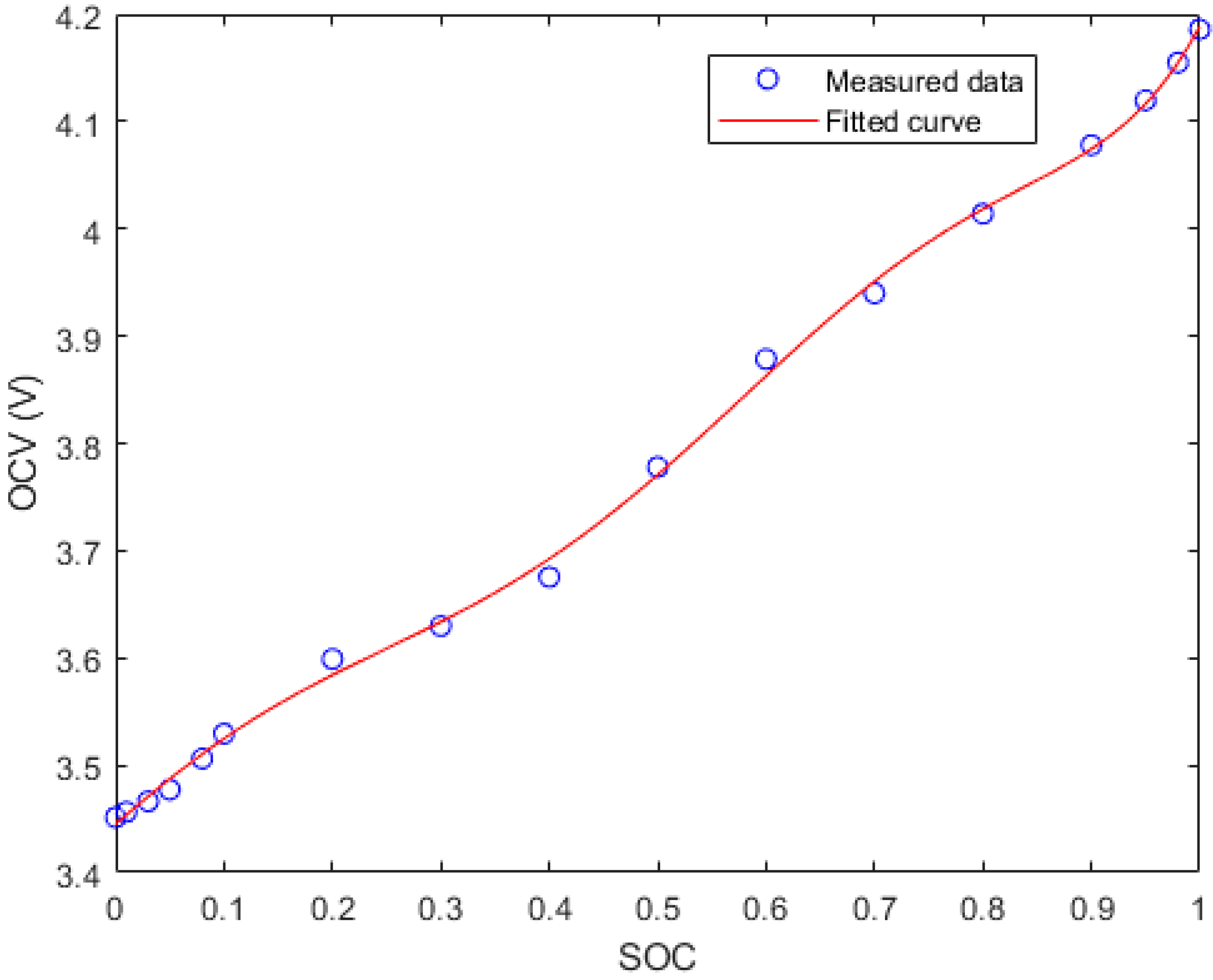
2.1. Battery Model Building and Offline Parameter Identification

As mentioned in the introduction, the electrochemical model and ECM are widely used as models of Li-ion battery. The electrochemical model is too complex for online parameter identification. Therefore, as shown in Figure 1, the Thevenin model (first-order ECM), which consists of an ideal voltage source, a resistor, and a resistor–capacitor (RC) network, is used in this study. $u_{\mathrm{oc}}$ indicates the OCV of the battery, while $u_{\mathrm{t}}$ represents the terminal voltage. $u_{\mathrm{p}}$ is the transient voltages of the RC network and $R_0$ describes the internal ohmic resistance of the battery.

The model can be expressed as following discrete state equations:

$$u_{\mathrm{oc}}(k+1)=u_{\mathrm{t}}(k+1)+i(k+1)R_0+u_{\mathrm{p}}(k+1)$$

(1)

$$u_{\mathrm{p}}(k+1)=u_{\mathrm{p}}(k)e^{-T/{\tau }_{\mathrm{s}}}+R_{\mathrm{p}}i(k)(1-e^{-T/{\tau }_{\mathrm{s}}})$$

(2)

where, T represents the sampling period and ${\tau }_{\mathrm{s}}=R_{\mathrm{p}}{C}_{\mathrm{p}}$ indicates the characteristic of the RC network.

Before the BMS works, the model parameters must be identified. A commonly-used method, pulse discharge process which is used for offline identification is described in [33].

Discharge the battery at a constant current I until the battery is stable. A step change of the current from $i$ = $I$ to $i$ = 0 will lead to a step change of the terminal voltage $\Delta u$, because the voltage across the ohmic resistor R₀ is abruptly changed to zero.

$$R_0=\left|\frac{\Delta u}{I}\right|$$

(3)

After that, in a long rest period of the battery, the terminal voltage, u_t, is expressed by the following exponential function:

$$u_{\mathrm{t}}=u_{\mathrm{oc}}-I{R}_{\mathrm{p}}{e}^{-t/R_{\mathrm{p}}{C}_{\mathrm{p}}}$$

(4)

On the basis of the measured terminal voltage data for each second in the rest period, the parameters R_p and C_p are obtained by the nonlinear fit of exponential function. In this study, it is calculated using Function nlinfit in MATLAB R2018a.

2.2. Online Parameter Identification using Improved SAVPSO

In a canonical PSO algorithm, each particle in the swarm stands for a potential solution to the specific problem, and the closeness to the target solution is expressed as a fitness function, for the Thevenin model, as shown in formula (8). The velocity of the particle indicates the rate and magnitude of the change in the battery model parameters. In order to achieve the optimization, the velocity of each particle is dynamically adjusted, according to the movement experience of itself and others.

There are three parameters to be identified in the Thevenin model. Thus, in the three-dimensional target search space, a swarm consists of $F$ particles $\left[1,2,\cdots ,f,\cdots F\right]$. The position of the $f$ particle is $x_f=[x_{f,R_0},x_{f,R_{\mathrm{p}}},x_{f,C_{\mathrm{p}}}]={[R_0,R_{\mathrm{p}},C_{\mathrm{p}}]}_{particle-f}$, and its velocity is $v_f=[v_{f,R_0},v_{f,R_{\mathrm{p}}},v_{f,C_{\mathrm{p}}}]$. The optimal position searched by the $f$ particle is $p_f=[p_{f,R_0},p_{f,R_{\mathrm{p}}},p_{f,C_{\mathrm{p}}}]$, while the optimal position searched by the whole swarm is expressed as $g=[g_{R_0},g_{R_{\mathrm{p}}},g_{C_{\mathrm{p}}}]$. The particle velocity and position update process in a canonical PSO is as following:

$$v_f(k+1)=\omega v_f(k)+c_1{r}_1(p_f(k)-x_f(k))+c_2{r}_2(g(k)-x_f(k))$$

(5)

$$x_f(k+1)=x_f(k)+v_f(k+1)$$

(6)

$$\omega ={\omega }_{\max }-k({\omega }_{\max }-{\omega }_{\min })/k_{\max }$$

(7)

$$\epsilon =\left|u_{\mathrm{t}}(k)-{\widehat{u}}_{\mathrm{t}}(k)\right|$$

(8)

where, $u_{\mathrm{t}}(k)$ and ${\widehat{u}}_{\mathrm{t}}(k)$ are the measured and estimated values of the battery terminal voltage. $c_1$ and $c_2$ are the influence coefficients about the current optimal and the history optimal. $r_1$ and $r_2$ indicates a random number between 0 and 1. $\omega$, ${\omega }_{\max }$ and ${\omega }_{\min }$ are inertia weight, maximum inertia weight, and minimum inertia weight, respectively. When ${\omega }_{\max }$ = 0.9, ${\omega }_{\min }$ = 0.1, the algorithm has stronger global search ability at the initial stage of iteration, and in the latter part of the iteration the algorithm tends to be more accurate for local search.

In order to improve the global search capability and the local search ability of the swarm, a random search mechanism related to the iteration step size is introduced on the basis of the canonical PSO—the SAVPSO algorithm [34]. The particle velocity update process in the SAVPSO is as following:

$$v_f(k+1)=\omega \left|p_{f^{\prime }}(k)-p_f(k)\right|sign(v_f(k))+r_1(p_f(k)-x_f(k))+r_2(g(k)-x_f(k))$$

(9)

where, $f^{\prime }$ means the random integer of $[0,F]$. Setting $c_1$ and $c_2$ as 1 and $r_1=1-r_2$ prevents the particles from searching too far from the feasible region, but that depends on the initialization of particles. $\omega \left|p_{f^{\prime }}(k)-p_f(k)\right|sign(v_f(k))$ changes with the search scope, and the global search ability of the algorithm is improved. In addition, in the later stage of the search, when the particles aggregate to the optimal solution, the particle iteration step size becomes smaller, which results in the strong local search ability of the algorithm, and that means fast convergence of the particle swarm.

The SAVPSO algorithm adjusts the randomness spontaneously according to the iterative step size of the particle. Therefore, when initialization and velocity update, the uniform random distribution of particles is very important. Without that, the ergodicity of swarm becomes poor in application, making it easy to fall into local optimum. In other words, poor ergodicity leads to instability of the identification results. In order to overcome its disadvantages, the algorithm process has been improved as follows:

(a) The velocity and position of a particle swarm is initialized using a piecewise logistic chaotic map, which can be expressed as:

$$e_f(k+1)=\{\begin{array}{l}4\mu e_f(k)(0.5-e_f(k))\begin{array}{cc},& 0\le e_f(k)\end{array}<0.5\\ 1-4\mu (1-e_f(k))(e_f(k)-0.5)\begin{array}{cc},& e_f(k)\end{array}\ge 0.5\end{array}$$

(10)

where, $e_f=[e_{f,R_0},e_{f,R_{\mathrm{p}}},e_{f,C_{\mathrm{p}}}]$ and $e_{f,R_0},e_{f,R_{\mathrm{p}}},e_{f,C_{\mathrm{p}}}\in (0,1)$. $\mu \in (0,4)$ is the control factor. At the beginning of chaotic initialization, a $F\times 3$ dimensional matrix $E=[e_1,e_2,\cdots ,e_f,\cdots ,e_F]$ is randomly generated and iterated through (10) until $k=F$. Then $e_f$ is mapped to the range of parameters $(-r_f,r_f)$, obtaining the initial velocity and position of the swarm:

$${e^{\prime }}_f=r_f(2e_f-1)$$

(11)

(b) To prevent the swarm from falling into local optimum, the covariance matrix of each particle’s position $\Delta ={\sigma }_{f,D}(f=1,2,\cdots ,n;D=1,2,3)$ is used to indicate the degree of aggregation. When $\Delta <\eta$ ($\eta$ is the specified small value, the swarm will be reinitialized by (10) and (11). Meanwhile, each dimension of each particle’s position has a probability (always set lower than 10%) of the mutation, which means to be changed into a random number between 0 and 1. Each particle only mutates in at most one dimension after each update.

(c) Replace $r_1$ and $r_2$ with a uniform random number between 0 and 1: $r_{unif}(0,1)$ to enhance the organizational autonomy of speed learning of each generation. Finally, the velocity update of improved SAVPSO algorithm is expressed as:

$$v_f(k+1)=\omega \left|p_{f^{\prime }}(k)-p_f(k)\right|sign(v_f(k))+c_1{r}_{unif}(0,1)(p_f(k)-x_f(k))+c_2{r}_{unif}(0,1)(g(k)-x_f(k))$$

(12)

The particles should not overstep the searching boundary $(L{B}_x,U{B}_x)$ or the velocity boundary $(L{B}_v,U{B}_v)$. When they do, they will be restricted at the boundary.

$$v_f(k+1)=\{\begin{array}{l}L{B}_v\begin{array}{cc}& v_f(k+1)<L{B}_v\end{array}\\ U{B}_v\begin{array}{cc}& v_f(k+1)>U{B}_v\end{array}\end{array}$$

(13)

$$x_f(k+1)=\{\begin{array}{l}L{B}_x\begin{array}{cc}& v_x(k+1)<L{B}_x\end{array}\\ U{B}_x\begin{array}{cc}& v_x(k+1)>U{B}_x\end{array}\end{array}$$

(14)

As the optimization iteration proceeds, $\epsilon$ continues to reduce. Then the parameters are identified and updated, regardless of the constantly changing parameters during battery operation or aging.

3. Joint Algorithm for SOC/SOH Online Estimation

3.1. Application of UKF for SOC Estimation

A Kalman filter consists of a prediction module and an error correction module [6]. For a nonlinear discrete system, its state space equation can be expressed as:

$$x_k=f\left(x_{k-1}\right)+w_{k-1}$$

(15)

$$z_k=h\left(x_k\right)+v_k$$

(16)

where, $x_k\in R^n$ is an unobservable state vector while $z_k\in R^n$ can be observed. $f(x)$ and $h(x)$ are known nonlinear equations. $w_{k-1}\in R^n$ represents process noise with a covariance matrix $Q_{n-1}$, while $v_k\in R^m$ means measurement noise with a covariance matrix of $R_k$.

In order to linearize the known nonlinear equations $f(x)$ and $h(x)$, unscented transform (UT) must be conducted. For nonlinear equation $z$ and (2n + 1) sample points of its random variable $x\in R^n$:

$$z=g\left(x\right)$$

(17)

$$\{\begin{array}{l}{\xi }_0=\overline{x}\\ {\xi }_i=\overline{x}+{\left(\sqrt{\left(n+\lambda \right)P_x}\right)}_i ,i=1,2,\cdots ,n\\ {\xi }_i=\overline{x}-{\left(\sqrt{\left(n+\lambda \right)P_x}\right)}_{i-n} ,i=n+1,n+2,\cdots ,2n\end{array}$$

(18)

where, $\overline{x}$ and $P_x$ are the mean and the covariance of $x$, respectively. With the constant $\alpha \in [0.0001,1]$, $\lambda ={\alpha }^2\left(n+\kappa \right)-n$ is a parameter used to adjust the diffusion degree of the sampling points. $\kappa =0$ will be set for the estimated state, while $\kappa =3-n$ will be set for the estimated parameter.

The mean and covariance of $z$ are expressed as:

$$\overline{z}={\displaystyle \sum _{i=0}^{2n}{w}_i^{\left(m\right)}g\left({\xi }_i\right)}$$

(19)

$$P_z={\displaystyle \sum _{i=0}^{2n}{w}_i^{\left(c\right)}\left(g\left({\xi }_i\right)-\overline{z}\right)}{\left(g\left({\xi }_i\right)-\overline{z}\right)}^{\mathrm{T}}$$

(20)

where, $w_i^{\left(m\right)}$ and $w_i^{\left(c\right)}$ are the weights for mean and covariance, respectively. With $\beta =2$ for the Gaussian distribution of variable $x$:

$$\{\begin{array}{l}{w}_0^{\left(m\right)}=\frac{\lambda }{n+\lambda }\\ w_0^{\left(c\right)}=\frac{\lambda }{n+\lambda }+1-{\alpha }^2+\beta \\ w_i^{\left(m\right)}=w_i^{\left(c\right)}=\frac{1}{2\left(n+\lambda \right)} ,i=1,2,\cdots ,2n\end{array}$$

(21)

The state space equation of the Thevenin model is expressed as:

$$x\left(k\right)=\left(\begin{array}{cc}1& 0\\ 0& 1-\frac{T}{C_{\mathrm{p}}{R}_{\mathrm{p}}}\end{array}\right)x\left(k-1\right)+\left(\begin{array}{l}-\frac{T}{C_{\mathrm{n}}}\\ \frac{T}{C_{\mathrm{p}}}\end{array}\right)i\left(k\right)$$

(22)

$$u_{\mathrm{t}}\left(k\right)=u_{\mathrm{oc}}\left(k\right)-i\left(k\right)R_0-u_{\mathrm{p}}\left(k\right)$$

(23)

$$x\left(k\right)=\left(\begin{array}{l}\mathrm{SOC}\left(k\right)\\ u_{\mathrm{p}}\left(k\right)\end{array}\right)$$

(24)

where, $C_n$ indicates the available capacity of the battery and there is a nonlinear relationship between $u_{oc}(k)$ and $SOC(k)$.

$$\mathrm{SOC}(t)=\mathrm{SOC}(t_0)-\frac{{\displaystyle {\int }_{t_0}^{t}i\mathrm{d}t}}{C_{\mathrm{n}}}$$

(25)

$$u_{\mathrm{oc}}\left(k\right)=f\left[\mathrm{SOC}\left(k\right)\right]$$

(26)

UKF is started from the step of initialization:

$${\widehat{x}}_0=E\left[x_0\right]$$

(27)

$$P_0=E\left[\left(x_0-{\widehat{x}}_0\right){\left(x_0-{\widehat{x}}_0\right)}^{\mathrm{T}}\right]$$

(28)

Then the prediction process is conducted:

$${\xi }_{k-1}=\left[{\overline{x}}_{k-1},{\overline{x}}_{k-1}+\left(\sqrt{\left(n+\lambda \right)P_{k|k-1}}\right),{\overline{x}}_{k-1}-\left(\sqrt{\left(n+\lambda \right)P_{k|k-1}}\right)\right]$$

(29)

$$X_{k|k-1}=f\left({\xi }_{k-1}\right)$$

(30)

$${\stackrel{⌒}{x}}_{k|k-1}={\displaystyle \sum _{i=0}^{2n}{w}_i^{\left(m\right)}{X}_{i,k|k-1}}$$

(31)

$$P_{k|k-1}={\displaystyle \sum _{i=0}^{2n}{w}_i^{\left(c\right)}}\left(X_{i,k|k-1}-{\widehat{x}}_{k|k-1}\right){\left(X_{i,k|k-1}-{\widehat{x}}_{k|k-1}\right)}^{\mathrm{T}}+Q_{k-1}$$

(32)

Subsequently, the error correction process must be finish:

$${\xi }_{k|k-1}=\left[{\stackrel{⌒}{x}}_{k|k-1},{\stackrel{⌒}{x}}_{k|k-1}+\left(\sqrt{\left(n+\lambda \right)P_{k|k-1}}\right),{\stackrel{⌒}{x}}_{k|k-1}-\left(\sqrt{\left(n+\lambda \right)P_{k|k-1}}\right)\right]$$

(33)

$${\stackrel{⌒}{z}}_{k|k-1}={\displaystyle \sum _{i=0}^{2n}{w}_i^{\left(m\right)}h\left({\xi }_{i,k|k-1}\right)}$$

(34)

$$P_{zz,k|k-1}={\displaystyle \sum _{i=0}^{2n}{w}_i^{\left(c\right)}\left(h\left({\xi }_{i,k|k-1}\right)-{\stackrel{⌒}{z}}_{k|k-1}\right){\left(h\left({\xi }_{i,k|k-1}\right)-{\stackrel{⌒}{z}}_{k|k-1}\right)}^{\mathrm{T}}+R_k}$$

(35)

$$P_{xz,k|k-1}={\displaystyle \sum _{i=0}^{2n}{w}_i^{\left(c\right)}\left({\xi }_{i,k|k-1}-{\stackrel{⌒}{x}}_{k|k-1}\right){\left(h\left({\xi }_{i,k|k-1}\right)-{\stackrel{⌒}{z}}_{k|k-1}\right)}^{\mathrm{T}}}$$

(36)

$$G_k=P_{xz,k|k-1}{P}_{zz,k|k-1}^{-1}$$

(37)

$${\stackrel{⌒}{x}}_k={\stackrel{⌒}{x}}_{k|k-1}+G_k\left(z_k-{\stackrel{⌒}{z}}_{k|k-1}\right)$$

(38)

$$P_k=P_{k|k-1}-G_k{P}_{zz,k|k-1}{G}_k^{\mathrm{T}}$$

(39)

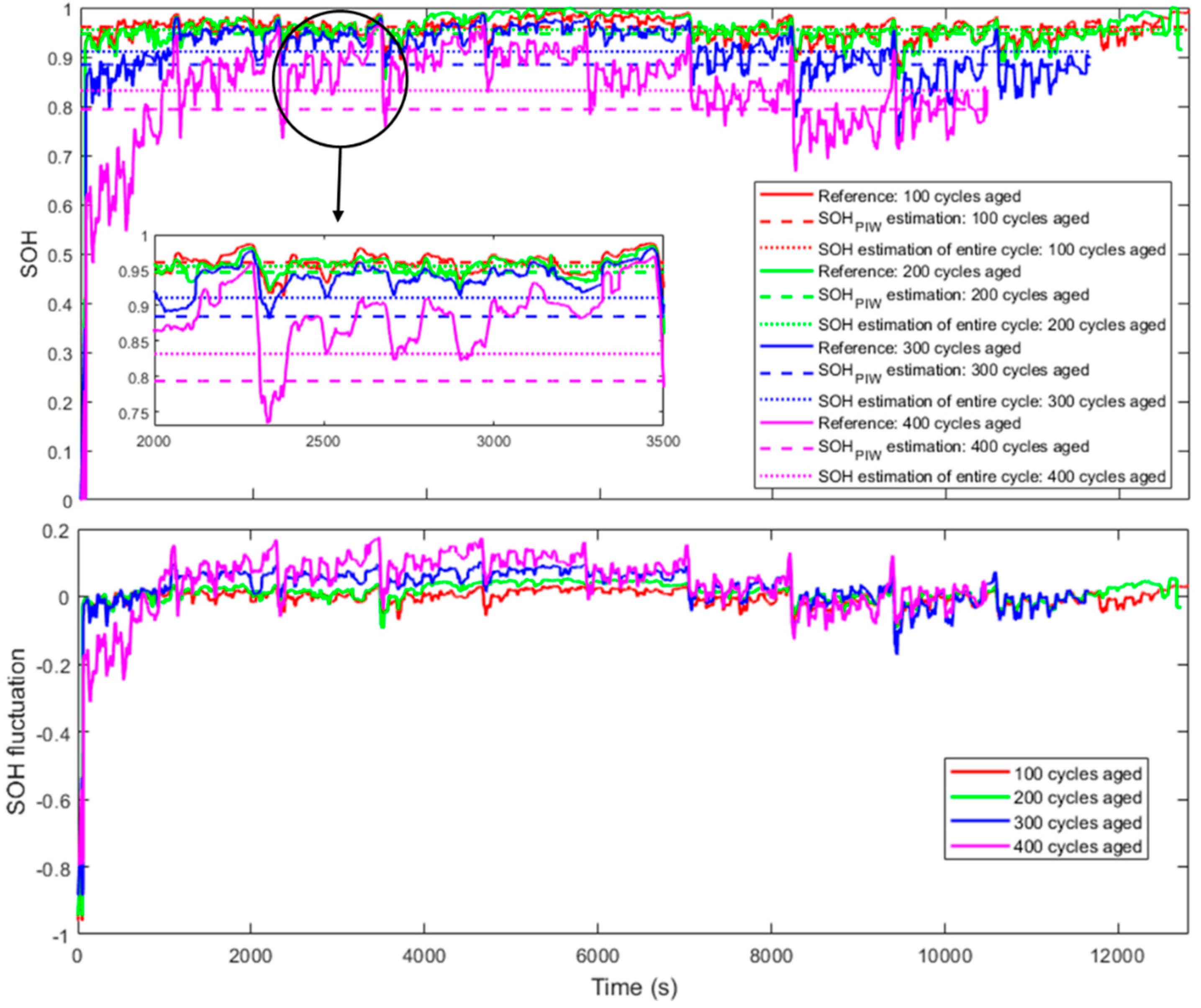
3.2. SOH Estimation Considering the Degree of Polarization

When the temperature of the working environment and the discharging rate are fixed, the polarization voltage, u_p, of new Li-ion batteries (ICR18650-22P) on the basis of the Thevenin model and its offline parameters, has the same changing trend as the SOC decrease, regardless of the SOC point at which the battery starts to discharge, as shown in Figure 2a. When the discharging rate increases, the amplitude of u_p increases but still maintains the same trend, as shown in Figure 2b. This phenomenon also exists when charging the batteries.

By selecting the polarization voltages of 0.2C discharging process (CC mode) and 0.5 C charging process (CCCV mode) at 25 °C as the reference values and conducting the linear interpolation, the standard polarization voltage (ups) of each point of SOC is obtainable, as shown in Figure 2c,d.

A new concept named degree of polarization (DOP) is proposed, which means the ratio between instantaneous polarization voltage and the standard polarization voltage at the corresponding SOC:

$$DOP(SOC)=u_{\mathrm{p}}(SOC)/u_{\mathrm{ps}}(SOC)$$

(40)

$$u_{\mathrm{p}}(SOC,k)=u_{\mathrm{oc}}(SOC(k))-u_{\mathrm{t}}(k)-i(k)R_0$$

(41)

The SOH of batteries is calculated from the available capacity ratio between the aged battery and the fresh battery:

$$SOH=\frac{C_{\mathrm{n},\mathrm{Aged}}}{C_{\mathrm{n},\mathrm{Fresh}}}$$

(42)

In the aging tests (25 °C, 1 C discharging for 400 cycles) of Li-ion batteries (ICR18650-22P), there is a linear relationship between the SOH and the mean absolute value of DOP in a single cycle, as shown in Figure 3. The linear relationship fitting is expressed as:

$$SO{H}_{\mathrm{cycle},\mathrm{cc}}=ar\frac{{\displaystyle \sum _{j=1}^n}\left|DOP\right|}{n}+b$$

(43)

where, $a$ and $b$ are constant coefficients, while $r$ is the ratio of 1 C discharge current to actual discharge current. When the actual discharge current is 1 C, there is $r=1$, which changes with the acquisition current. $n$ represents number of data in one cycle.

With 95% confidence bounds (-0.03097, -0.02459) and (0.9988, 1.024), the constant coefficients a and b are settled, as shown in

Table 3. The identification of constant coefficients $a$ and $b$.

$a$	$b$
−0.02778	1.011

.

So far, the DOP realizes the SOH estimation under constant current operation of each cycle. To achieve real-time estimation of arbitrary conditions, this study introduces the parameter identification window (PIW), which is used to store a piece of data with a fixed data length (the data length of PIW in this study equals 100), indicating the operation data in a short period. With a new pair of measured values (current and terminal voltage) collected, the PIW moves forward to the new data, without changing the data length. For the data in PIW, $x_j$ is a random sample from an unknown distribution of SOH:

$$x_j= |\frac{i_{1\mathrm{C}}}{i(k)}DOP(k)|\cdot a+b$$

(44)

According to a kernel density estimator [35], for estimated values $S\stackrel{⌒}{O}{H}_{\mathrm{PIW}}$, the probability density function in PIW is expressed as:

$${\stackrel{⌒}{f}}_{\mathrm{h}}(S\stackrel{⌒}{O}{H}_{\mathrm{PIW}}(k))=\frac{1}{Nh}\sum _{j=1}^{N}K(\frac{S\stackrel{⌒}{O}{H}_{\mathrm{PIW}}(k)-x_j}{h})$$

(45)

$$\max \left\{{\stackrel{⌒}{f}}_{\mathrm{h}}(S\stackrel{⌒}{O}{H}_{\mathrm{PIW}}(k))\right\}\to S\stackrel{⌒}{O}{H}_{\mathrm{PIW}}(k)$$

(46)

where, $K$ means the kernel smoothing function, and $h$ is the bandwidth of kernel density, while $N=100$ means the data length of PIW. When the probability density function in PIW ${\stackrel{⌒}{f}}_{\mathrm{h}}(S\stackrel{⌒}{O}{H}_{\mathrm{PIW}}(k))$ takes the maximum value, the corresponding independent variable is the SOH estimated value. Thus, the SOH can be identified online as the PIW moves forward.

It should be noted that the frequent changes of SOH in one cycle (meaning that the available capacity changes many times each cycle) will lead to jumps of the SOC estimated results or divergence of the SOC estimation algorithm. Therefore, the solution is that the SOH should be updated only once per cycle, and the updated value is the mean of all the PIWs’ SOH estimates:

$$S\stackrel{⌒}{O}{H}_{\mathrm{cycle}}=\frac{{\displaystyle \sum _{k=1}^n}S\stackrel{⌒}{O}{H}_{\mathrm{PIW}}(k)}{n}$$

(47)

3.3. Design of the Joint Algorithm

According to the above principles, when BMS works, the parameters of the Thevenin model are identified online by the improved SAVPSO algorithm. The UKF estimates the SOC of batteries based on dynamic model parameters, while DOP monitors and updates the SOH online.

In actual working conditions, the charging and discharging current rate of batteries has great uncertainty. When the vehicle sensor collects current and terminal voltage, there will be measurement noise, and the ambient temperature will change constantly. With the proposed SAVPSO-UKF algorithm (see blue background block in Figure 4), the parameters of the model are updated in real time and the measurement noise is filtered, regardless of the aforementioned interference factors. However, after battery aging, the available capacity of the battery decreases, and online parameter identification becomes difficult to determine. As the monitoring of battery DOP in the PIW moves forward (see pink background block in Figure 4), the available battery capacity is estimated online and the SOH of battery is updated each cycle.

Figure 4 illustrates the steps of the proposed joint algorithm:

① Initialize algorithm and load battery offline test data;

② The battery operating current and terminal voltage are collected with measurement noise for online parameter identification. Output RC parameters and terminal voltage are estimated;

③ Based on the identified parameters, the SOC is estimated;

④ SOH of corresponding PIW is calculated;

⑤ PIW moves forward and the algorithm is set back to step ②, until operating current data flow stops;

⑥ SOH and the available capacity of the entire cycle are updated.

4. Experiments and Discussion

4.1. Experiments Configuration

As shown in Figure 5, the experimental setup consists of four parts:

Part 1 The Li-ion battery, Samsung ICR18650-22P, LiCoO₂, nominal voltage 3.6 V, nominal capacity 2.15 Ah, end voltage 2.75 V and 4.2 V.

Part 2 The battery operating system, Arbin (BT-5HC), voltage range 0–5 V, maximum current 30 A, accuracies of current and voltage ±0.02%.

Part 3 The temperature controlling chamber, Sanwood, range -40°C to 150°C, accuracy ±0.1°C.

Part 4 The signal and data processing tool, MATLAB R2018a unit in a host computer.

The voltage and current are measured and sent to the host computer each second for the verification of algorithm.

The battery experiment schedule is divided into two parts, offline tests and online tests, as shown in Figure 6.

The offline tests are, mainly, to obtain the actual capacity of the battery, offline parameters of the Thevenin model, and the OCV-SOC curve. The offline experimental methods are found in [31].

With the conditions of 25 °C, 0.5 C charging (CCCV mode) and 0.2 C discharging (CC mode), the average actual capacity of this batch is 2.1318 Ah.

A hybrid pulse power characteristic (HPPC) test is completed as follows: (1) The battery to be tested is fully charged by CCCV and allowed to rest for 2 h, then the terminal voltage is measured and recorded as the OCV of the battery at SOC = 1; (2) the battery is discharged to SOC = 0.98 at 0.2 C and rest for 2 h, the terminal voltage is recorded as the OCV of the battery at SOC = 0.98; (3) step 2 is repeated to determine the OCV of the battery at SOC = 0.95, 0.9, 0.8, 0.7, 0.6, 0.5, 0.4, 0.3, 0.2, 0.1, 0.08, 0.05, 0.03, 0.01, and 0, separately. Afterwards, the OCV-SOC curve is determined by fitting the data points with the sixth-order polynomial, as shown in Figure 7.

The HPPC test contains 16 pulse discharge processes required for identification of offline parameters [33], with the conditions of 25 °C, the pulse discharge process of 100% SOC to 98% SOC, and its rest period according to formulae (3) and (4). The offline parameters of the Thevenin model are identified as shown in

Table 4. Offline parameter identification results of the Thevenin model.

$R_0$	$R_{\mathrm{p}}$	$C_{\mathrm{p}}$
0.0367	0.0183	3768.0211

.

When it comes to online battery tests, in order to verify that the proposed algorithm can be applied to complex road conditions and have high estimation accuracy and robustness, regardless the changes in discharging current rate and working temperature, we designed an estimation test with combined variable temperature and operating condition, as shown in Figure 8.

In order to verify that the proposed algorithm still functions after the battery ages, the battery is subjected to an aging experiment. Here, for the reliability of the experimental results, it is necessary to avoid abnormal damage to the battery due to excessive temperature changes and current fluctuation. Thus, this study proposes constant current cyclic aging and New European Driving Cycle (NEDC) tests; the steps are shown in Figure 9. At 25 °C, the battery is tested in the NEDC mode every 50 times after constant current charging and discharging, until the actual available capacity is less than 80%.

The measurement noises are very small when high-precision sensors are used in the laboratory experiments to collect current and voltage data, but there are accuracy limits of current and voltage sensors onboard. For the purpose of verifying the noise robustness of the proposed algorithm, noises are added to the current and voltage data to simulate actual operating conditions.

When preparing current for estimation, Gaussian white noise with mean 0 A and variance 10–2 A is added to the experiment data as a sensor error. As for terminal voltage, Gaussian white noise with mean 0 V and variance 10–4 V is added.

4.2. Estimation Results of Variable Temperature Combined Operating Condition Test

Under the combined operating current profile (see Figure 10a) and with the working temperature profile (see Figure 10b), the terminal voltages of the proposed method and the UKF can be output, respectively (see Figure 10c), while the voltage errors are shown in Figure 10d. The maximum error of the output terminal voltage of the proposed method based on online parameter identification is 43.47 mV, and the average error is 8.03 mV. When it comes to UKF (using the offline parameters in Table 4), the maximum error is up to 366.80 mV, and the average error is 50.50 mV. This indicates that the proposed algorithm can realize online parameter identification according to different operating conditions and dramatically changing the working temperature of batteries (shifting between 5–45 °C), ensuring the accuracy of the battery model.

The SOC estimation result is shown in Figure 10e. The black line indicates the reference SOC values, which were computed by the Ampere-hour counting method using experimental data from the Arbin battery test system. It is noted that, using the proposed method, the maximum error is about 1% of an entire cycle, as shown in Figure 10f.

In this study, DOP, which indicates the degree of electrochemical polarization and concentration polarization of the Li-ion battery, is the basic parameter for the SOH estimation. As shown in Figure 10g, DOP changes steadily with the operating condition and working temperature profiles in Figure 10a,b. The battery DOP is always higher when the ambient temperature is lower or the discharging current is larger, leading to a longer charging time and a shorter battery life.

Under the operation condition in Figure 10a,b, the SOH estimation results are shown in Figure 10h. The SOH_PIW, the red line in Figure 10h, indicates the health status of the battery in real time. It should be noted that the real-time estimation of SOH drops significantly when the battery is operated at a large operating current in a low-temperature environment; this explains why battery life will be compromised when a vehicle always runs at a low temperature, using a large discharging current for climbing. However, the SOH is more stable when the temperature is higher than room temperature (25 °C) and the current fluctuation is small. Compared with the reference (SOH = 93.104%) obtained offline from experiments, the SOH estimation value of the entire cycle based on the proposed algorithm is 91.319%, which indicates an error of estimation of 1.785%.

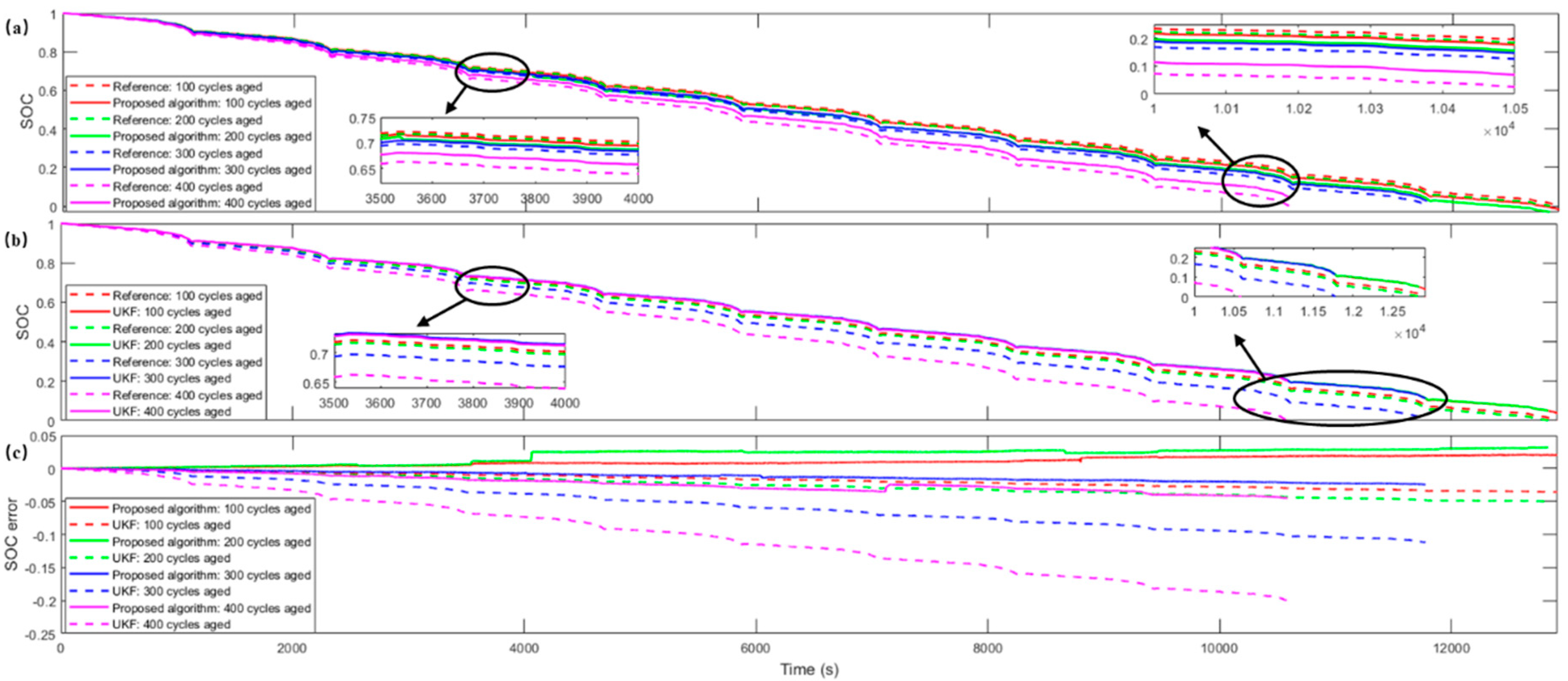
4.3. Estimation Results of the Constant Current Cyclic Aging and the NEDC Tests

As shown in Figure 11, the proposed algorithm can improve the accuracy of the SOC estimation in the whole life cycle of the battery in actual operating condition. The maximum SOC estimation error is about 4.5% from battery online service to retirement.

Compared with the UKF algorithm, the proposed algorithm identifies the model parameters online and updates the available capacity of the battery according to the degree of polarization. Therefore, no matter how the battery is in the environment and how aged it is, this method can estimate the SOC more accurately, as shown in Figure 11. The comparisons of mean and maximum error are shown in

Table 5. Comparison of the SOC estimation errors in aging process.

Aging Cycles	Mean Error of Proposed Method	Mean Error of UKF	Maximum Error of Proposed Method	Maximum Error of UKF
100	1.02%	1.78%	2.06%	3.58%
200	1.94%	2.58%	3.17%	4.99%
300	1.19%	5.60%	2.44%	11.20%
400	2.22%	9.83%	4.51%	20.03%

.

The DOP-SOC curves in the aging process, as shown in Figure 12, indicates that the degree of polarization of aged batteries will be much greater than that of new batteries while working, which means large terminal voltage loss and poor Li-ion movement inside the battery, leading to severe battery heating, and even thermal runaway. When the SOC value is between zero and 0.2, or greater than 0.9, the DOP value is also larger. When the discharging process begins, the Li-ion quickly embeds into the cathode, running out of residual Li-ion at the cathode electrolyte and cathode surface, while it needs more time for the movement of Li-ion from anode electrolyte and anode surface, then the DOP rises. When the discharging process runs out of Li-ion from the anode electrolyte and the anode surface, while it needs more time for the movement of Li-ion from active material inside the anode, then the DOP rises as well.

The reference of SOH_PIW is calculated based on (43), using the aging experimental data collected from high-precision sensors. It is noted that during battery discharge, the real-time estimated SOH fluctuates around the exact value as the operating conditions change. As the battery ages, the stability of the electrochemical reaction inside the battery decreases, which causes the battery’s SOH to be more susceptible to working conditions, resulting in a larger fluctuation, as shown in Figure 13. The maximum SOH estimation error of the entire cycle in the aging process is about 3.82%, as shown in

Table 6. SOH estimation error of entire cycle in the aging process.

Aging Cycles	100	200	300	400
SOH error of entire cycle	0.58%	0.87%	2.64%	3.82%

.

5. Conclusions

On the basis of the commonly used Thevenin model, this study introduces an improved SAVPSO algorithm, using UKF to ensure the accuracy of the SOC estimation. The concept of degree of polarization is defined as the ration between instantaneous polarization voltage and the standard polarization voltage at the corresponding SOC. Furthermore, real-time SOH estimation and cyclic update of the SOH in the battery life cycle are achieved based on the degree of polarization, using a kernel density estimator. To verify the proposed method, a series of experiments, including a variable temperature combined operating condition test and NEDC tests in the whole aging processes of batteries, are conducted. The experimental results show that the proposed joint algorithm enhances the SOC estimation accuracy in the full battery life cycle with the cyclic update of SOH, even in cases of operating aged batteries and under complex operating conditions. The maximum SOC estimation error is about 4.5% from battery online service to retirement, while the maximum SOH estimation error is about 3.82% in the aging process.

References

1. Cuma, M.U.; Koroglu, T. A comprehensive review on estimation strategies used in hybrid and battery electric vehicles. Renew. Sustain. Energy Rev. 2015, 42, 517–531. [Google Scholar] [CrossRef]
2. Farmann, A.; Waag, W.; Marongiu, A.; Sauer, D.U. Critical review of on-board capacity estimation techniques for lithium-ion batteries in electric and hybrid electric vehicles. J. Power Sources 2015, 281, 114–130. [Google Scholar] [CrossRef]
3. Zou, Y.; Hu, X.; Ma, H.; Li, S.E. Combined State of Charge and State of Health estimation over lithium-ion battery cell cycle lifespan for electric vehicles. J. Power Sources 2015, 273, 793–803. [Google Scholar] [CrossRef]
4. Ng, K.S.; Moo, C.S.; Chen, Y.P.; Hsieh, Y.C. Enhanced coulomb counting method for estimating state-of-charge and state-of-health of lithium-ion batteries. Appl. Energy 2009, 86, 1506–1511. [Google Scholar] [CrossRef]
5. Ng, K.S.; Moo, C.S.; Chen, Y.P.; Hsieh, Y.C. State-of-Charge Estimation for Lead-acid Batteries Based on Dynamic Open-circuit Voltage. In Proceedings of the IEEE International Power & Energy Conference, Johor Bahru, Malaysia, 1–3 December 2008. [Google Scholar]
6. Yatsui, M.W.; Bai, H. Kalman Filter Based State-of-Charge Estimation for Lithium-ion Batteries in Hybrid Electric Vehicles Using Pulse Charging. In Proceedings of the Vehicle Power and Propulsion Conference, Chicago, IL, USA, 6–9 September 2011; pp. 1–5. [Google Scholar]
7. Tian, Y.; Xia, B.; Sun, W.; Xu, Z.; Zheng, W. A modified model based state of charge estimation of power lithium-ion batteries using unscented Kalman filter. J. Power Sources 2014, 270, 619–626. [Google Scholar] [CrossRef]
8. Zou, Z.; Xu, J.; Mi, C.; Cao, B.; Chen, Z. Evaluation of Model Based State of Charge Estimation Methods for Lithium-Ion Batteries. Energies 2014, 7, 5065–5082. [Google Scholar] [CrossRef] [Green Version]
9. Yun, Z.; Zhang, C.; Zhang, X. State-of-charge estimation of the lithium-ion battery system with time-varying parameter for hybrid electric vehicles. IET Control Theory Appl. 2013, 8, 160–167. [Google Scholar]
10. Zhou, F.; Wang, L.; Lin, H.; Lv, Z. High Accuracy State-of-Charge Online Estimation of EV/HEV Lithium Batteries Based on Adaptive Wavelet Neural Network. In Proceedings of the Ecce Asia Downunder, Melbourne, Australia, 3–6 June 2013. [Google Scholar]
11. Shi, Q.; Zhang, C.; Cui, N.; Zhang, X. Battery State-of-Charge Estimation in Electric Vehicle Using Elman Neural Network Method. In Proceedings of the Control Conference, Beijing, China, 29–31 July 2010. [Google Scholar]
12. Liu, R.H.; Sun, Y.K.; Ji, X.F. Battery State of Charge Estimation for Electric vehicle Based on Neural Network. In Proceedings of the International Conference on Information & Computer Networks, Xi′an, China, 27–29 May 2011. [Google Scholar]
13. Xu, J.; Cao, B.; Zheng, C.; Zou, Z. An online state of charge estimation method with reduced prior battery testing information. Int. J. Electr. Power Energy Syst. 2014, 63, 178–184. [Google Scholar] [CrossRef]
14. Hui, B.; Yang, Y. State of Charge Estimation for Electric Vehicle Batteries Based on LS-SVM. In Proceedings of the International Conference on Intelligent Human-machine Systems & Cybernetics, Hangzhou, China, 26–27 August 2013. [Google Scholar]
15. Xia, B.; Chen, C.; Tian, Y.; Sun, W.; Xu, Z.; Zheng, W. A novel method for state of charge estimation of lithium-ion batteries using a nonlinear observer. J. Power Sources 2014, 270, 359–366. [Google Scholar] [CrossRef]
16. Sepasi, S.; Roose, L.; Matsuura, M. Extended Kalman Filter with a Fuzzy Method for Accurate Battery Pack State of Charge Estimation. Energies 2015, 8, 5217–5233. [Google Scholar] [CrossRef]
17. Kim, J.; Lee, S.; Cho, B.H. Complementary Cooperation Algorithm Based on DEKF Combined With Pattern Recognition for SOC/Capacity Estimation and SOH Prediction. IEEE Trans. Power Electron. 2011, 27, 436–451. [Google Scholar] [CrossRef]
18. Hu, Y.; Yurkovich, S. Battery State of Charge Estimation in Automotive Applications Using LPV Techniques. In Proceedings of the American Control Conference, Baltimore, MD, USA, 30 June–2 July 2010. [Google Scholar]
19. Han, X.; Ouyang, M.; Lu, L.; Li, J.; Zheng, Y.; Li, Z. A comparative study of commercial lithium ion battery cycle life in electrical vehicle: Aging mechanism identification. J. Power Sources 2014, 251, 38–54. [Google Scholar] [CrossRef]
20. Fu, R.; Choe, S.Y.; Agubra, V.; Fergus, J. Modeling of degradation effects considering side reactions for a pouch type Li-ion polymer battery with carbon anode. J. Power Sources 2014, 261, 120–135. [Google Scholar] [CrossRef]
21. Schmidt, A.P.; Bitzer, M.; Imre, Á.W.; Guzzella, L.J. Model-based distinction and quantification of capacity loss and rate capability fade in Li-ion batteries. J. Power Sources 2010, 195, 7634–7638. [Google Scholar] [CrossRef]
22. Hu, X.; Li, S.E.; Jia, Z.; Egardt, B. Enhanced sample entropy-based health management of Li-ion battery for electrified vehicles. Energy 2014, 64, 953–960. [Google Scholar] [CrossRef]
23. Zheng, Y.; Han, X.; Lu, L.; Li, J.; Ouyang, M. Lithium ion battery pack power fade fault identification based on Shannon entropy in electric vehicles. J. Power Sources 2013, 223, 136–146. [Google Scholar] [CrossRef]
24. Saha, B.; Kai, G.; Poll, S.; Christophersen, J. Measurement, Prognostics Methods for Battery Health Monitoring Using a Bayesian Framework. IEEE Trans. Instrum. Meas. 2009, 58, 291–296. [Google Scholar] [CrossRef]
25. Eddahech, A.; Briat, O.; Bertrand, N.; Delétage, J.Y.; Vinassa, J.M. Behavior and state-of-health monitoring of Li-ion batteries using impedance spectroscopy and recurrent neural networks. Int. J. Electr. Power Energy Syst. 2012, 42, 487–494. [Google Scholar] [CrossRef]
26. Qiang, M.; Lei, X.; Cui, H.; Wei, L.; Pecht, M. Remaining useful life prediction of lithium-ion battery with unscented particle filter technique. Microelectron. Reliab. 2013, 53, 805–810. [Google Scholar]
27. Sbarufatti, C.; Corbetta, M.; Giglio, M.; Cadini, F. Adaptive prognosis of lithium-ion batteries based on the combination of particle filters and radial basis function neural networks. J. Power Sources 2017, 344, 128–140. [Google Scholar] [CrossRef]
28. Klass, V.; Behm, M.; Lindbergh, G.J. A support vector machine-based state-of-health estimation method for lithium-ion batteries under electric vehicle operation. J. Power Sources 2014, 270, 262–272. [Google Scholar] [CrossRef]
29. Zenati, A.; Desprez, P.; Razik, H.; Rael, S. A Methodology to Assess the State of Health of Lithium-ion Batteries Based on the Battery′s Parameters and a Fuzzy Logic System. In Proceedings of the Electric Vehicle Conference, Greenville, SC, USA, 4–8 March 2012. [Google Scholar]
30. Guha, A.; Patra, A. State of Health Estimation of Lithium-Ion Batteries Using Capacity Fade and Internal Resistance Growth Models. IEEE Trans. Transp. Electrif. 2017, 4, 135–146. [Google Scholar] [CrossRef]
31. Xia, B.; Lao, Z.; Zhang, R.; Tian, Y.; Chen, G.; Sun, Z.; Wang, W.; Sun, W.; Lai, Y.; Wang, M.; et al. Online Parameter Identification and State of Charge Estimation of Lithium-Ion Batteries Based on Forgetting Factor Recursive Least Squares and Nonlinear Kalman Filter. Energies 2018, 11, 3. [Google Scholar] [CrossRef]
32. Shi, Y.; Eberhart, R.C. Empirical Study of Particle Swarm Optimization. In Proceedings of the 1999 Congress on Evolutionary Computation-CEC99, Washington, DC, USA, 6–9 July 1999. [Google Scholar]
33. Schweighofer, B.; Raab, K.M.; Brasseur, G. Modeling of high power automotive batteries by the use of an automated test system. IEEE Trans. Instrum. Meas. 2003, 52, 1087–1091. [Google Scholar] [CrossRef]
34. Lu, H.; Chen, W.J. Self-adaptive velocity particle swarm optimization for solving constrained optimization problems. J. Glob. Optim. 2008, 41, 427–445. [Google Scholar] [CrossRef]
35. Ghorai, J.K.; Susarla, V. Kernel estimation of a smooth distribution function based on censored data. Metrika 1990, 37, 71–86. [Google Scholar] [CrossRef]
Figure 1. The Thevenin model.
Energies 12 02939 g001
Figure 2. The polarization voltage (up) SOC curves of discharging processes and the standard polarization voltage curves (25 °C). (a) With different starting SOC points, (b) with different discharging current rates, (c) ups for discharging process, and (d) ups for charging process.
Energies 12 02939 g002
Figure 3. The linear fitting between the SOH and the mean |degree of polarization (DOP)| (25 °C, 1 C cyclic charging and discharging until the available capacity reaches 80%)
Energies 12 02939 g003
Figure 4. Schematic of the joint algorithm.
Energies 12 02939 g004
Figure 5. The experiment configuration.
Energies 12 02939 g005
Figure 6. The schedule of experiments.
Energies 12 02939 g006
Figure 7. The measured and fitted OCV-SOC curve at 25 °C.
Energies 12 02939 g007
Figure 8. Combined variable temperature and operating condition.
Energies 12 02939 g008
Figure 9. The steps of constant current cyclic aging and NEDC tests.
Energies 12 02939 g009
Figure 10. Estimation results of the variable temperature combined operating condition test. (a) Operating current profile combined by Urban Dynamometer Driving Schedule (UDDS), Dynamic Stress Test (DST), NEDC, and Federal Urban Driving Schedule (FUDS); (b) working temperature profile shifting between 5–45 °C; (c) output terminal voltages; (d) terminal voltages error; (e) estimated SOC; (f) SOC error; (g) DOP-SOC curve; and (h) Estimated SOHPIW and estimated SOH of entire cycle.
Energies 12 02939 g010
Figure 11. The SOC estimation results in aging process. (a) Estimated SOC of proposed method, (b) estimated SOC of unscented Kalman filter (UKF), and (c) SOC errors.
Energies 12 02939 g011
Figure 12. The DOP-SOC curves in the aging process.
Energies 12 02939 g012
Figure 13. The SOH estimation results and SOH fluctuation in the aging process.
Energies 12 02939 g013