1. Introduction
One of the aims in current automotive development is to reduce the energy consumption of the vehicles, amongst others by reducing the aerodynamic drag. A substantial contribution to the aerodynamics drag comes from the air that passes through the cooling system for the driveline components. Hence, optimizing the size of the grille openings and underhood architecture for the necessary amount of cooling air flow helps improving the energy efficiency of the vehicle. Computational fluid dynamics (CFD) has been recognized as an important tool in the aerodynamic and thermal management development process of road vehicles, as it can be used in early stages when no physical prototype is available.
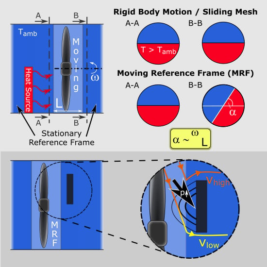
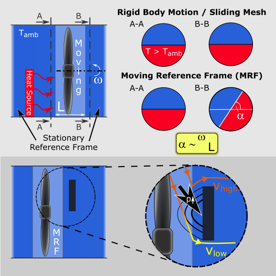
The modelling of moving parts is one of the major challenges when using CFD, since unsteady simulations are costly and time-consuming. A common way of modelling rotation is to use the so-called “multiple reference frame” (MRF) approach, which transforms the velocity components in a defined region around the rotating part to a rotating reference frame. Hence, instead of the blades moving physically through the air, the air moves around the rotor blades with a corresponding velocity. The MRF approach is relatively simple to implement and suitable for steady state simulations, which makes it a computationally inexpensive method. This approach is often used in industrial applications, such as cooling of electrical components [
1,
2], ventilation [
3,
4], tidal current turbines [
5,
6] and automotive applications. In the automotive industry, areas of application are, e.g., the rotation of wheels [
7] and of the fan for the cooling system.
However, there are limitations to this model. For instance, the fan performance curve, describing the pressure rise over volume flow rate through the fan, is commonly under-predicted when using the MRF model [
8]. This under-prediction mainly occurs at low to medium volume flow rates (radial and transitional regime [
9]), therefore it is concluded that the MRF method works best when the fan is operating in axial conditions. Liu et al. (2016) found that the thrust of a tidal current turbine was equally under-predicted with the MRF approach as the pressure rise. Furthermore, they found that the frozen rotor position has a significant influence on the flow field in the near wake [
6]. Kobayashi and Kohri (2011) showed that uniform inflow conditions are necessary in order to facilitate the transition to the moving reference frame [
10]. Apart from the operating conditions, it is also important that flow structures originating from the blades (e.g., tip vortices) are completely encompassed by the MRF domain, in order not to be split or in other ways being hindered from developing [
11]. A large MRF domain has therefore been shown to give better agreement with experimentally obtained fan curves [
12,
13,
14,
15]. For open fans (i.e., no ring connecting the blade tips), the radial extent is more important, due to the occurring tip vortices, while for both the open and closed fan type a sufficiently large axial extent can lead to more uniform inflow conditions and hence a better performance prediction. Therefore it can be concluded that the users choice of the MRF domain has a substantial impact on the accuracy of the results.
In spite of these limitations, the MRF persists in being a popular approach due to its computational efficiency. Most of the previous studies used the prediction of the fan performance curve as an indicator for the accuracy of the MRF approach. To the knowledge of the authors, no work has been published on the transport phenomena over the different reference frames. The purpose of this study is to investigate the effect of the MRF approach on non-uniform temperature and velocity fields around a typical vehicle cooling fan. Therefore, several numerical test cases are studied, in order to assess the influence of different MRF zone sizes, rotational rates and geometric obstructions in the domain up- and downstream of the MRF zone. The present investigation is purely numerical and the corresponding set-up run with an Rigid Body Motion approach serves as the reference for validation.
2. Methodology
2.1. Fan Modelling
There are three main approaches implemented in current commercial CFD solvers that can be used to simulate fan rotation: the lumped fan model (LF), the MRF model and the rigid body motion (RBM) model. The simplest of these three, and the only actual fan model, is the lumped fan model, which uses an interface at the location where the fan blades would be located. An experimentally obtained fan curve is then used to apply a pressure rise over the interface according to the mass flow rate. The drawbacks of this model are that the velocity vectors exiting the interface of the standard LF model only have an axial component, but no swirl and no reduced velocity where the hub would be located. These drawbacks can be reduced by adding a swirl to the outlet flow, or geometrically leaving out the hub region from the interface. However, it still is a simplified model that requires a-priori experimental results to get a proper output. This approach is currently mostly used in simulations of the cooling of electric components, due to their shorter development cycles. With increasing computational power more advanced models, such as the MRF, are becoming more common in those areas as well [
2].
The MRF model includes the geometry of the fan blades and therefore does not require any experimental data. It can be used in a steady state simulation, using a frozen rotor approach and transferring the velocities entering a user-defined region around the blades to a moving reference frame:
Here, is the velocity in the global (stationary) reference frame, the rotational vector and the position vector in the field of rotation. An important limitation of this approach is that the user-defined MRF domain needs to be rotational symmetric and must not contain any stationary, non-rotationally symmetric parts. In automotive applications, the fan is usually placed just a few centimetres downstream of the radiator, with the struts that are holding the fan and its motor, directly downstream of the fan blades. This limits the maximum available space to place an MRF region considerably. A large domain, as recommended by Gullberg and Kobayashi, can therefore usually not be achieved.
The RBM method is the most physically correct approach to use, since it actually performs the rotation. It requires an unsteady approach, where a domain containing the rotor geometry is rotated and interfaces are used to transfer information from the moving to the stationary domain. During the whole process, the mesh in each domain remains the same, sliding against each other. Therefore, this approach is often also referred to as the “sliding mesh” approach. In order to ensure a proper exchange of information over the interface, the degree of rotation per time step is restricted. Usually, a time step corresponding to a degree of rotation of
is recommended. Some cases might however allow for a larger time step size (e.g., Lim et al. (2018) [
16]). Depending on the application, the benefit of rotating the blades using the RBM approach and therefore obtaining a physically accurate solution can outweigh the high computational effort.
2.2. Governing Equations
The numerical simulations were performed with Simcenter StarCCM+ (Ver 13.06) by Siemens. The steady state (MRF) cases were run by solving the governing equations in their Reynolds-averaged Navier Stokes (RANS) formulation, and the unsteady cases (RBM) by solving the governing equations in their improved delayed detached eddy simulation (IDDES) formulation. The discretized governing equations (conservation equations for mass, momentum and energy) in their respective RANS or IDDES formulation can be found in literature, e.g., in [
17].
In the RANS formulation, an additional source term with new unknowns was introduced, the so-called Reynolds stress term. In order to close this system of equations, further equations were necessary in the form of turbulence models. For this study, a two-equation model was used, the realizable
k-
-model in a two layer approach. In this approach, the turbulent dissipation rate,
, was specified by a wall function in the near-wall region and in the freestream as a function of the turbulent kinetic energy,
k. This model was chosen for its simplicity and due to good applicability for rotating and swirling flows [
18].
The unsteady simulations that are performed as a reference to the steady state MRF simulations are carried out using an IDDES approach. IDDES is a hybrid turbulence model between RANS and Large Eddy Simulation (LES), and is therefore expected to yield more accurate results compared to RANS, given a sufficiently fine mesh resolution. As the name indicates, LES resolves the larger turbulent scales and models the smaller ones with the help of subgrid scale models (SGS). Simcenter provides three different subgrid scale models for DES to chose from, whereof only the Spalart–Allmaras SGS and the Shear-Stress-Transport (SST)
k-
model were available in IDDES formulation. For the present set-up, the Spalart–Allmaras model was chosen for the IDDES simulation, due to its known accuracy in boundary layer flows [
18].
2.3. Numerical Set-Up
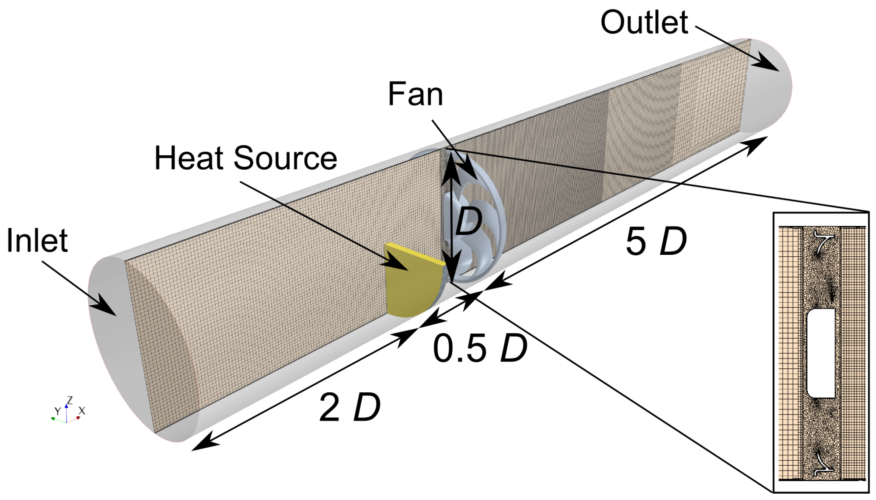
The computational domain is a long pipe, see
Figure 1. The pipe extends 2.5
D upstream of the MRF region and 5
D downstream, where
D is the diameter of the fan. The inlet boundary condition was set to a constant mass flow rate (
kg/s) and the outlet to a pressure outlet. The surrounding walls are set as walls with a non-slip condition. The fan is a vehicle axial cooling fan with eight forward-swept blades. In the fan region, the mesh was carefully constructed to retain the features of the fan blades, as well as to resolve the boundary layer around the blades. Therefore an initial simulation is performed to choose the right amount of prism layers (
) and the total prism layer thickness (
mm), in order to achieve
, suitable for the IDDES solver. In the next step, the base size of the volumetric cells in the air side was reduced by 20 % starting from 20 mm.
The mesh that was finally chosen for this study (M3,
Table 1) consisted of 2.65 million polyhedral cells in the fan region and 2.33 million trimmed cells in the remaining pipe, giving a total cell count of ≈5 million. This mesh was chosen since a further refinement (M4) did not show a considerable difference in the predicting the pressure rise over the fan and was computationally more expensive to run. The steady state simulations were assumed to be converged once all residuals have dropped and stabilized below
, and the pressure rise over the MRF interfaces has stabilized.
A heat source was placed 0.5 D upstream of the fan region, extending over the lower half of the pipe with a rejected heat of 5 kW. For this study, the magnitude of the heat source was not considered to be relevant, as long as it created a notable difference in temperature between the upper and the lower half of the computational domain. There was no porosity or other parameter set, so that the fluid was disturbed as little as possible by the heat source.
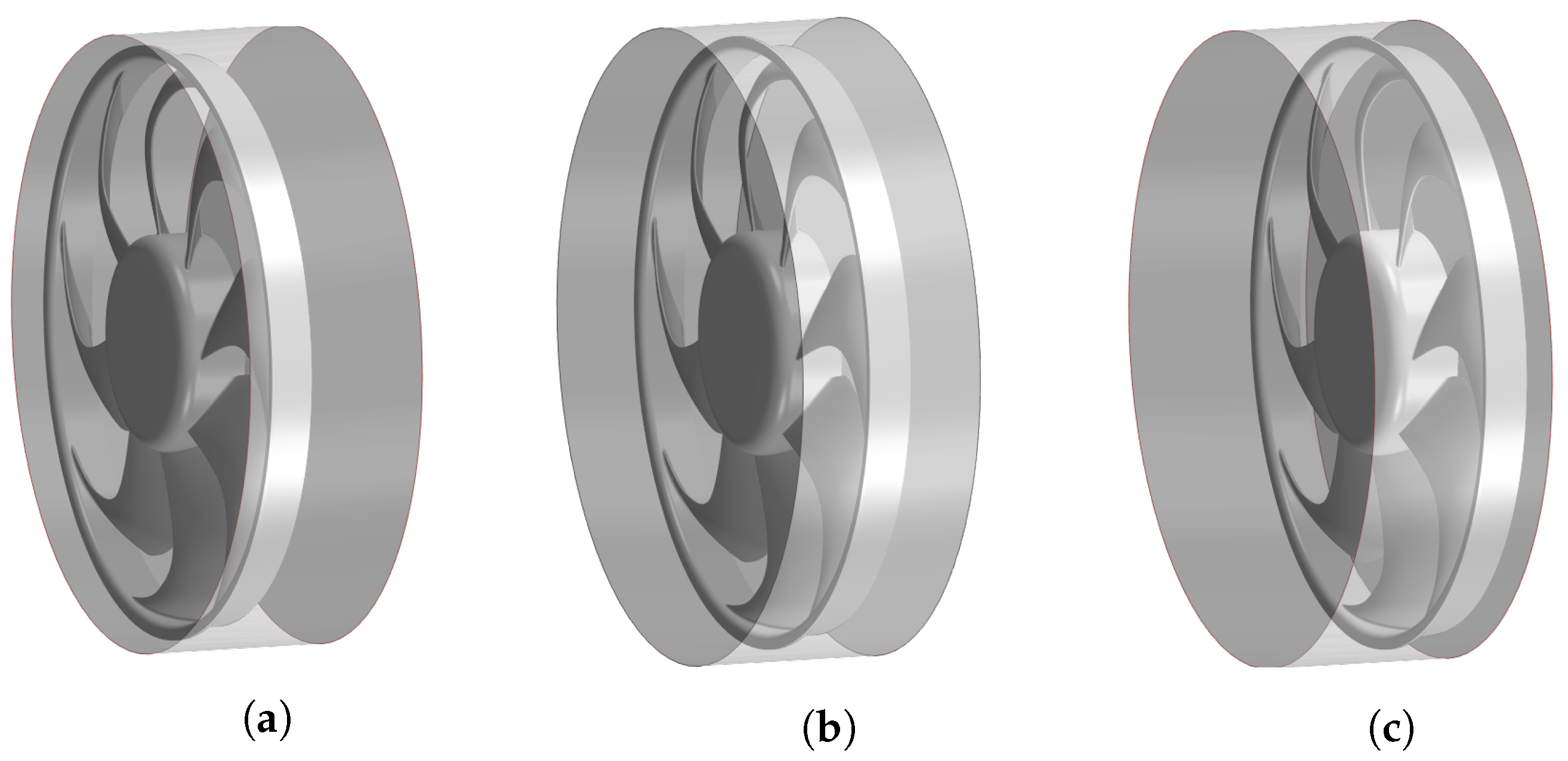
In the first part of the study, only the transport of the temperature field was investigated while varying different parameters (length of the MRF zone, rotational rate, blades/no blades). The baseline case had a length of the MRF region equal to
mm, and the fan rotated with a rotational rate of 2800 rpm. This fan speed was chosen since it was close to the maximum speed this type of fan would have in a typical passenger car installation. In case T1, the rotational rate was reduced to 1400 rpm while keeping the mass flow through the pipe constant, in order to investigate the effect the rotational rate has on the quantities of interest. In case T2, the rotational speed is again 2800 rpm but the MRF domain was extended to
mm, with varying blade positions (see
Figure 2). The purpose was to see if there is an influence of the distance between the MRF regions interfaces and the blades. In case T2(a) the fan blades were placed close to the upstream interface, in case T2(b) in the centrally between the up- and downstream interface and in case T2(c) close to the downstream interface.
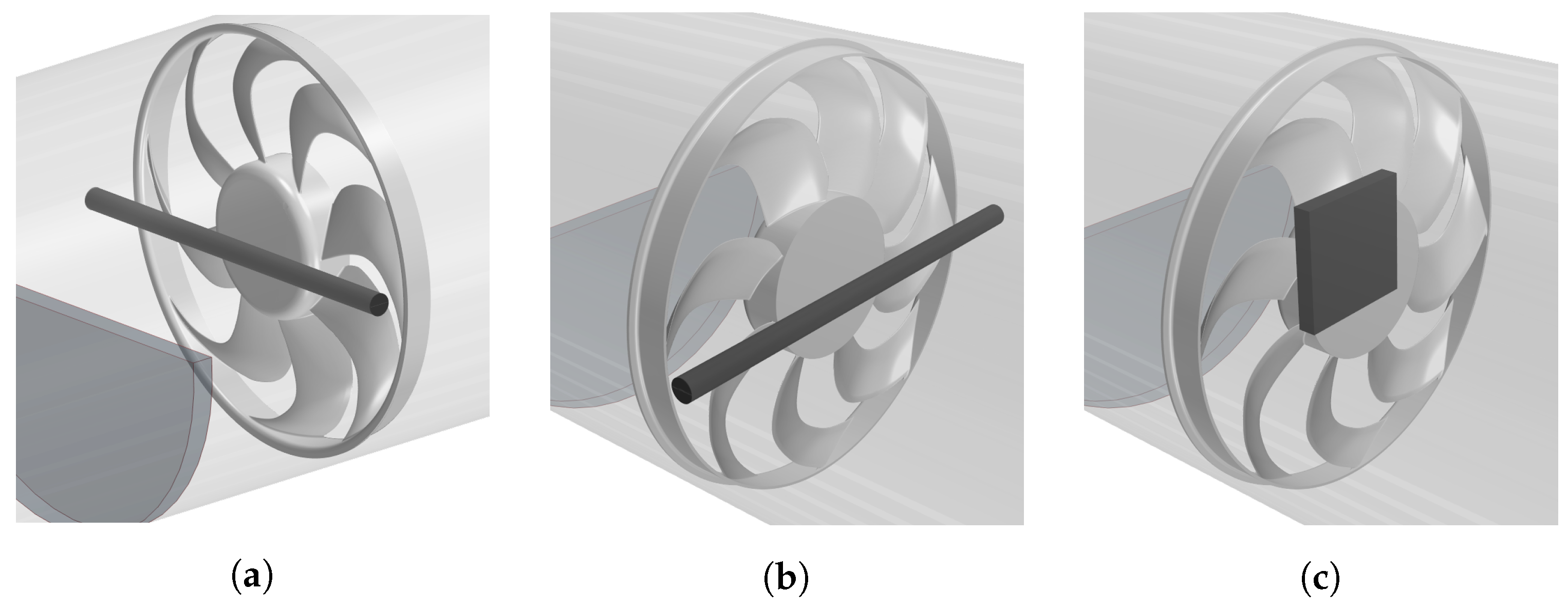
In the second part of the study it is investigated how non-uniformities in the flow field are transported through the fan domain. All cases were run with the baseline set-up (2800 rpm,
mm), with different obstructions being introduced into the flow: a cylinder (
m), which was once placed first upstream (case F1), then downstream (case F2) of the fan, and a box (
mm
, case F3) which was placed downstream of the fan region (see
Figure 3).
An overview of the investigated configurations can be found in
Table 2. All aforementioned cases also run without fan blades. In addition, the corresponding unsteady RBM simulations were performed and used for validation. This was a valid approach as it has been shown in previous studies, that the results obtained from an RBM simulation were sufficiently close to experimental data [
6,
19]. The RBM simulations were run with a time step of
s over a time corresponding to ten full rotations. The velocity, pressure and temperature fields were averaged after an initial transition period, from steady to unsteady, corresponding to three full rotations of the fan.
3. Results
The results are presented in two parts. First, the results from the temperature field investigation are presented. Second, the influence of geometric obstructions placed closely up- or downstream of the MRF region is investigated for the different configurations described in
Section 2.3.
3.1. Temperature Field
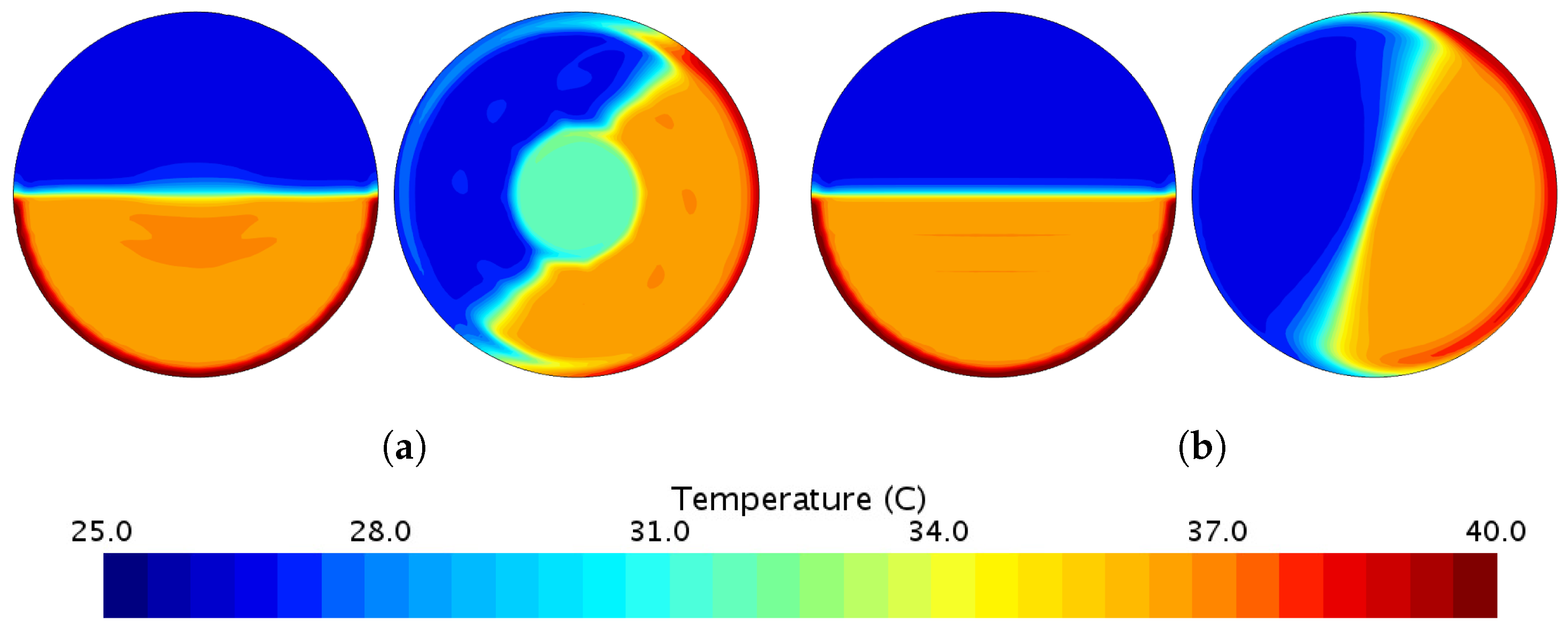
3.1.1. Baseline ( mm/2800 rpm)
Figure 4 shows the temperature field at the up- and downstream interface of the fan region including blades with the MRF approach (a) and the resulting temperature field obtained by using the rigid body motion (b). It can be observed that the temperature field in the MRF case has experienced a rotation of ≈90 deg, while the temperature field in the RBM simulation, as expected, did not rotate. Hence, the rotation of the temperature field is regarded as a non-physical effect.
For the case without the blade geometry present in the fan region, the angle of rotation of the temperature field increased to ≈140 deg (
Figure 4). This further illustrates the non-physicality of the observed rotational effect, since there were no components that could induce this rotation.
The reason for this effect can be seen in
Figure 5, which shows the streamlines of the relative velocity coloured by temperature. It can be observed that there were almost no temperature changes along the same streamline in the MRF case: the top two streamlines that do not pass through the heat source remain at ambient temperature throughout the whole MRF region, while the bottom two heat up due to the heat source, and then remain at that temperature. In the RBM case, the temperature along the streamlines changes according to their position in the global reference frame. Hence, it can be concluded that the temperature field is transported through the MRF region by means of the relative streamlines. In the RBM simulation, the temperature field is transported by the streamlines of the absolute velocity, and therefore the temperature field does not experience a notable rotation.
3.1.2. Case T1 ( mm/1400 rpm)
Figure 6 shows the results for case T1, which is the same configuration as the baseline case, but at a reduced rotational rate (1400 rpm). Since the rotational rate has decreased, the angle of rotation for the temperature field has decreased to approximately half of the degree of rotation in the previous case (≈50 deg). Removing the blades leads to half of the degree of rotation (≈70 deg) than the one that is observed for the baseline case without blades. Another case was investigated, where also the mass flow rate in the pipe had been reduced to half of the mass flow rate of the baseline case, in order to obtain the same relation between rotational rate and inflow velocity. It is observed that when reducing the mass flow rate at the pipes inlet boundary to 0.5 kg/s, the degree of rotation becomes identical to the baseline case, as the inflow conditions are comparable. Hence, it can be concluded that the angle of rotation depends on the inflow conditions, i.e., the ratio between axial velocity and the rotational rate of the fan.
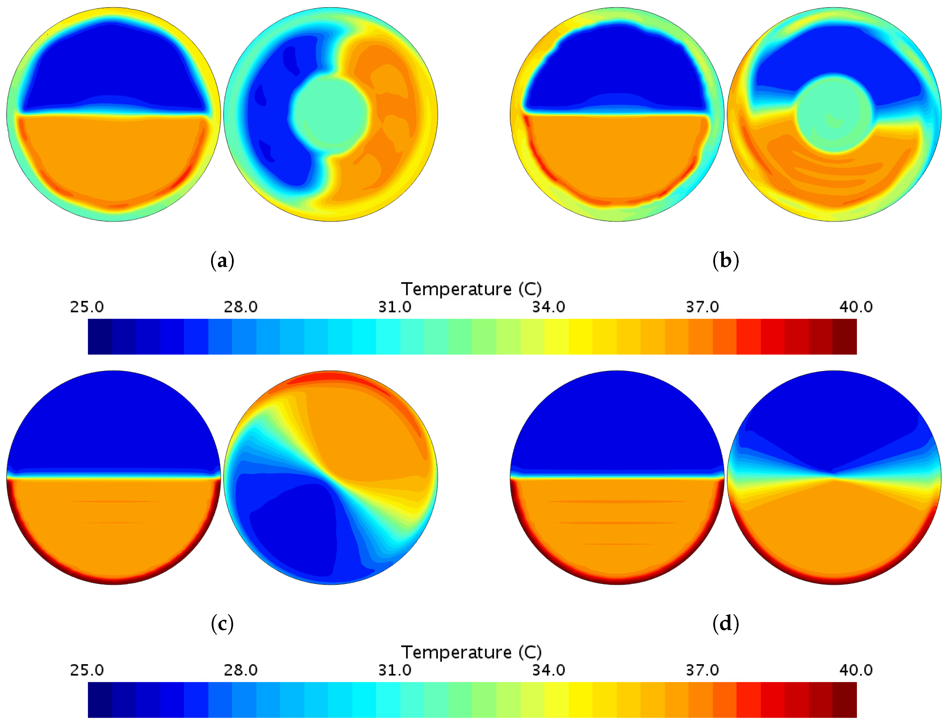
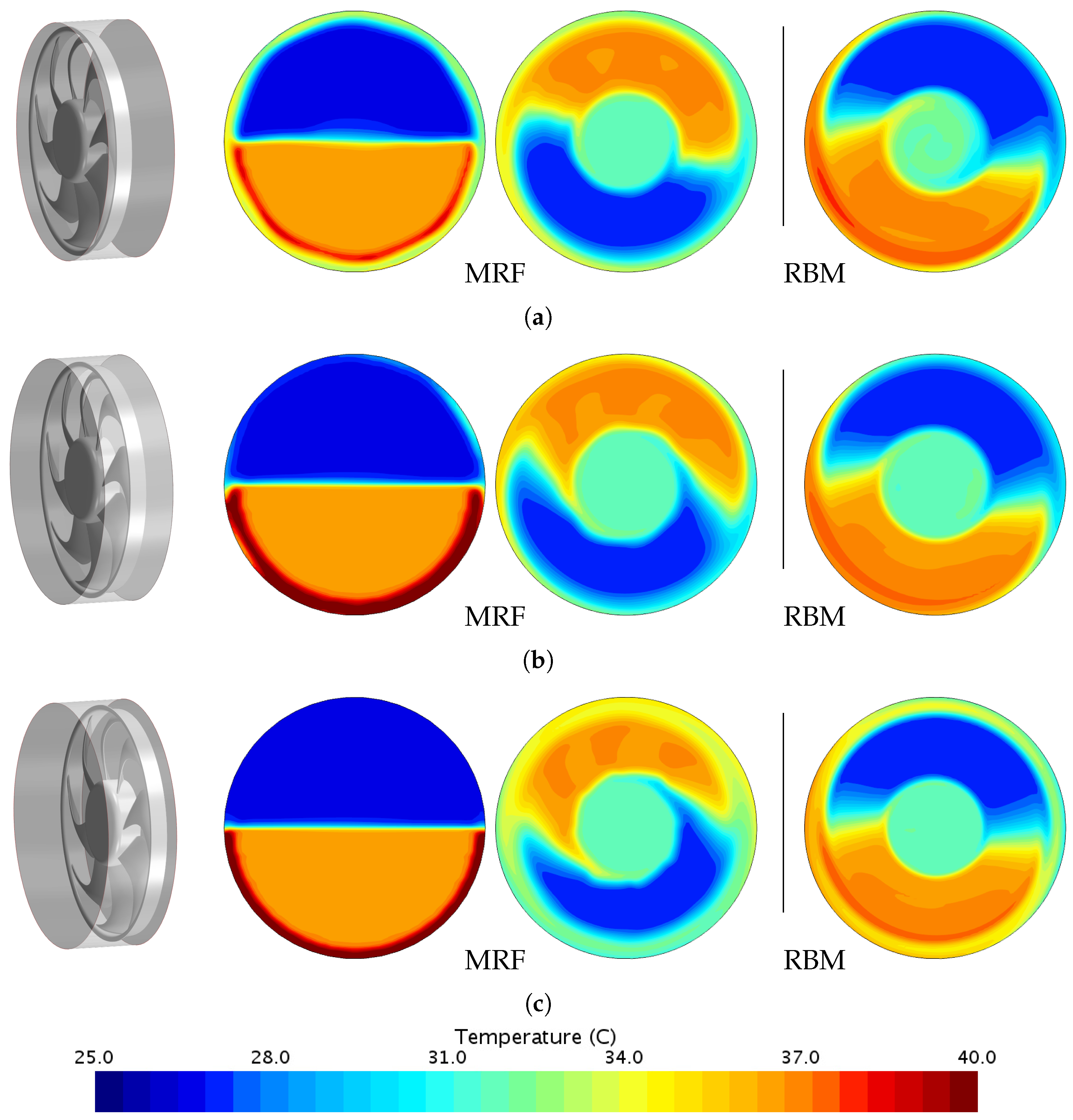
3.1.3. Case T2 ( mm/2800 rpm)
As was pointed out by Gullberg and Löfdahl (2011) [
13] and Kobayashi et al. (2014) [
14] the performance of the MRF approach is highly dependent on the users choice of the size of the MRF domain. To investigate how a larger MRF region affects the rotation of the temperature field, a region with
mm is studied. Additionally, an analysis of the impact of the rotors position in relation to the interfaces (see
Figure 2) is performed. The purpose of this part of the study is to determine if there is an effect of how much pre-rotation the flow experiences before hitting the blades. As can be seen in
Figure 7, the degree of rotation roughly doubles as compared to the baseline case (from 90 to
). Hence, it can be concluded that the degree of rotation is proportional to the length of the MRF domain. The temperature field was now shifted by ≈180 deg, independently on where the blades are located in the MRF domain. This means that the regions which should see a low temperature in reality were now considerably warmer, and vice versa. The positioning of the blades, however, only had a minor effect on the amount of rotation of the temperature field. The degree of rotation amounted to approximately 5 to
between the cases (a) and (b), and cases (b) and (c). These differences were marginal compared to the rotation that is caused by the length of the MRF domain in itself.
3.2. Flow Field
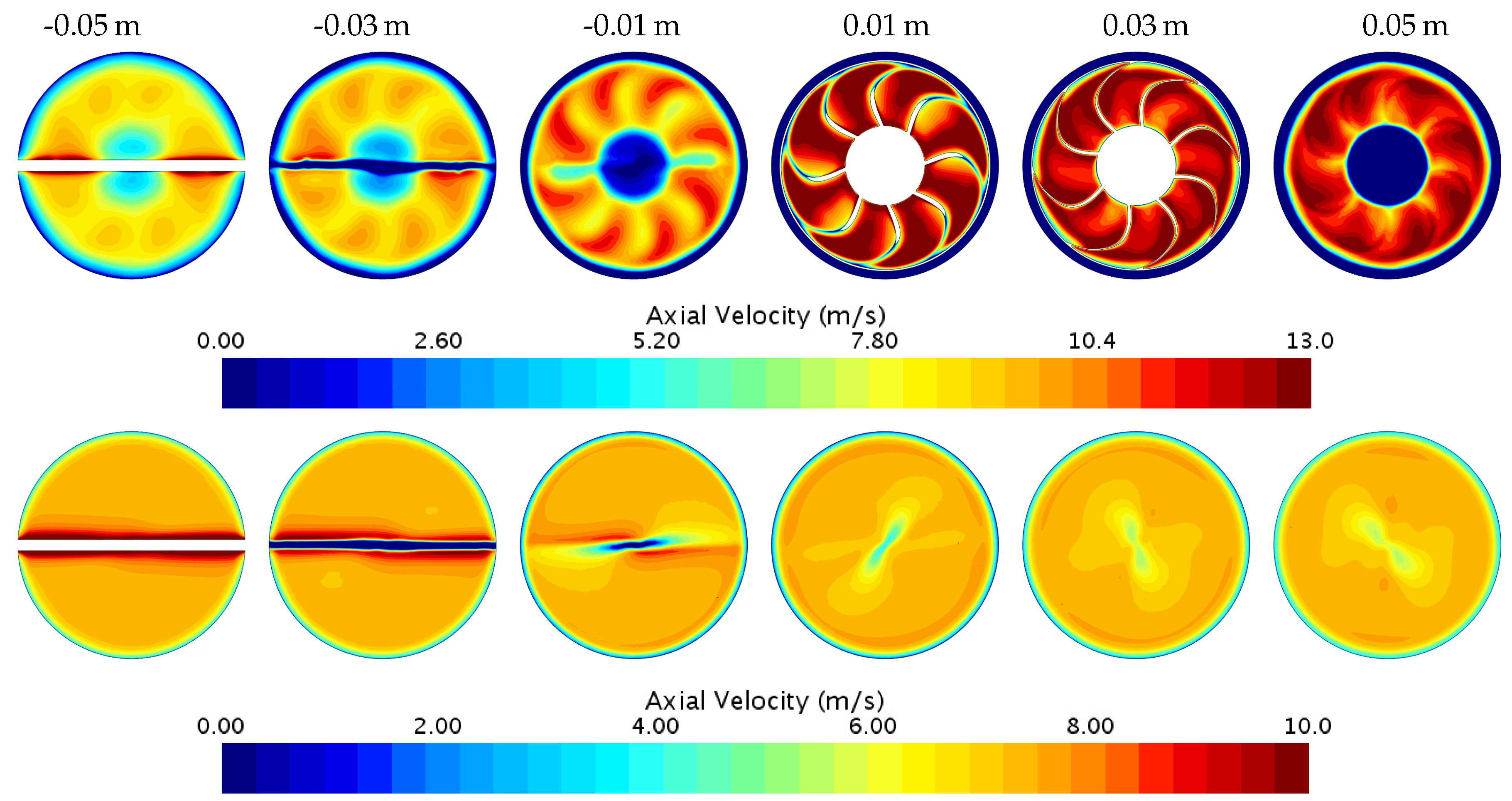
3.2.1. Case F1—Cylinder (Upstream)
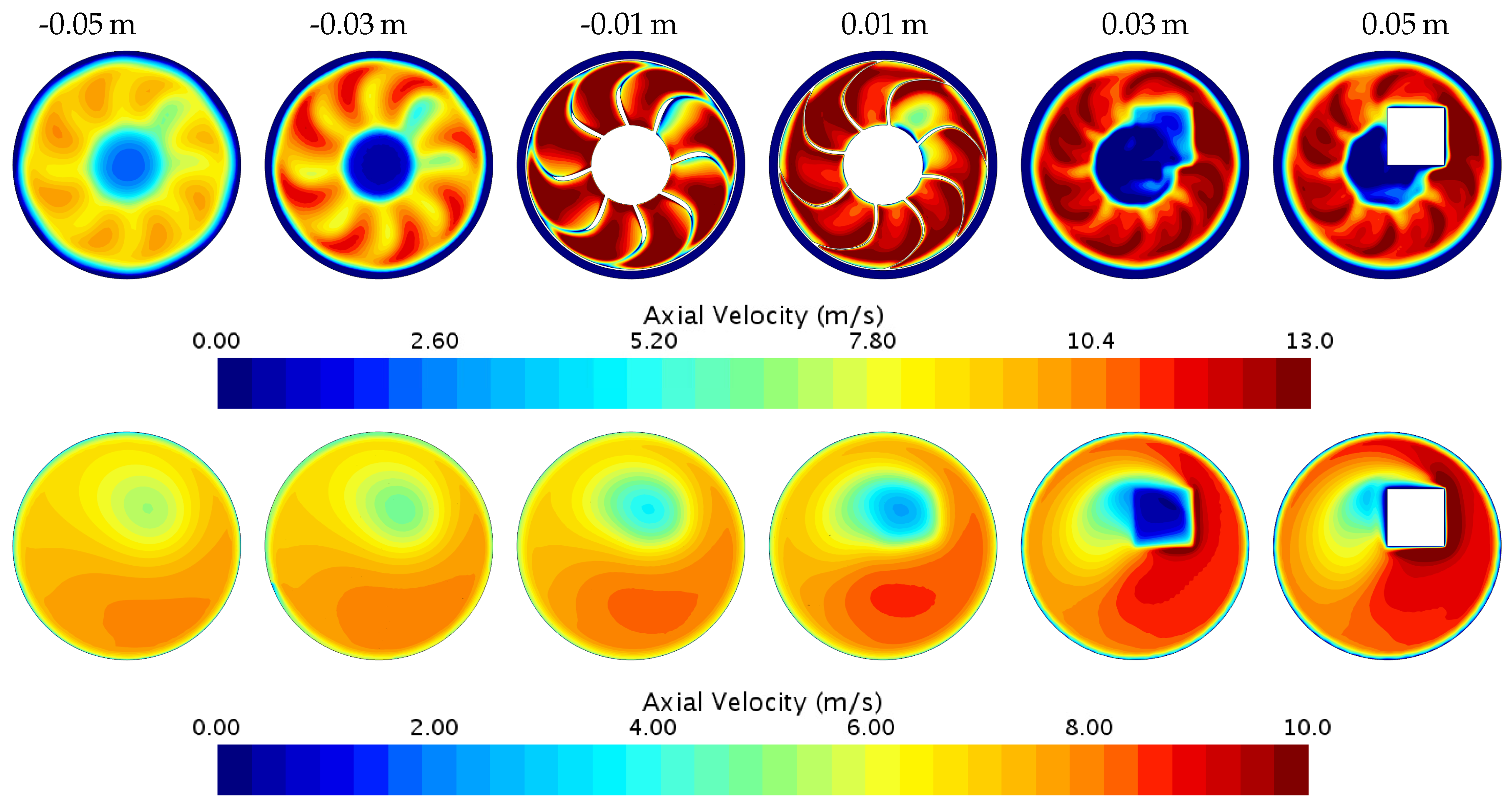
A cylinder with a diameter of
m was placed 1
d upstream of the interface to the fan region, extending over the complete width of the pipe. The results for the axial velocity component are presented in
Figure 8. The cross-sectional planes go from 0.05 m upstream to 0.05 m downstream of the fan blades (left to right). It can be observed that in the case without fan blades in the region (lower row), the wake of the cylinder starts to rotate as soon as it enters the MRF region (
m) and keeps on rotating until the end of the MRF region is reached (
m). The rotation was counter-clockwise and to the same degree as the temperature field in the previous section (≈140 deg). In the case with blades (upper row), the wake also starts to rotate when entering the fan region. Here, the rotation was difficult to trace throughout the length of the domain, since the wake of the cylinder is superposed by the wake of the fan blades. Hence, the effect on the downstream flow can be considered small.
3.2.2. Case F2—Cylinder (Downstream)
The results for placing the cylinder 1
d downstream of the MRF region can be seen in
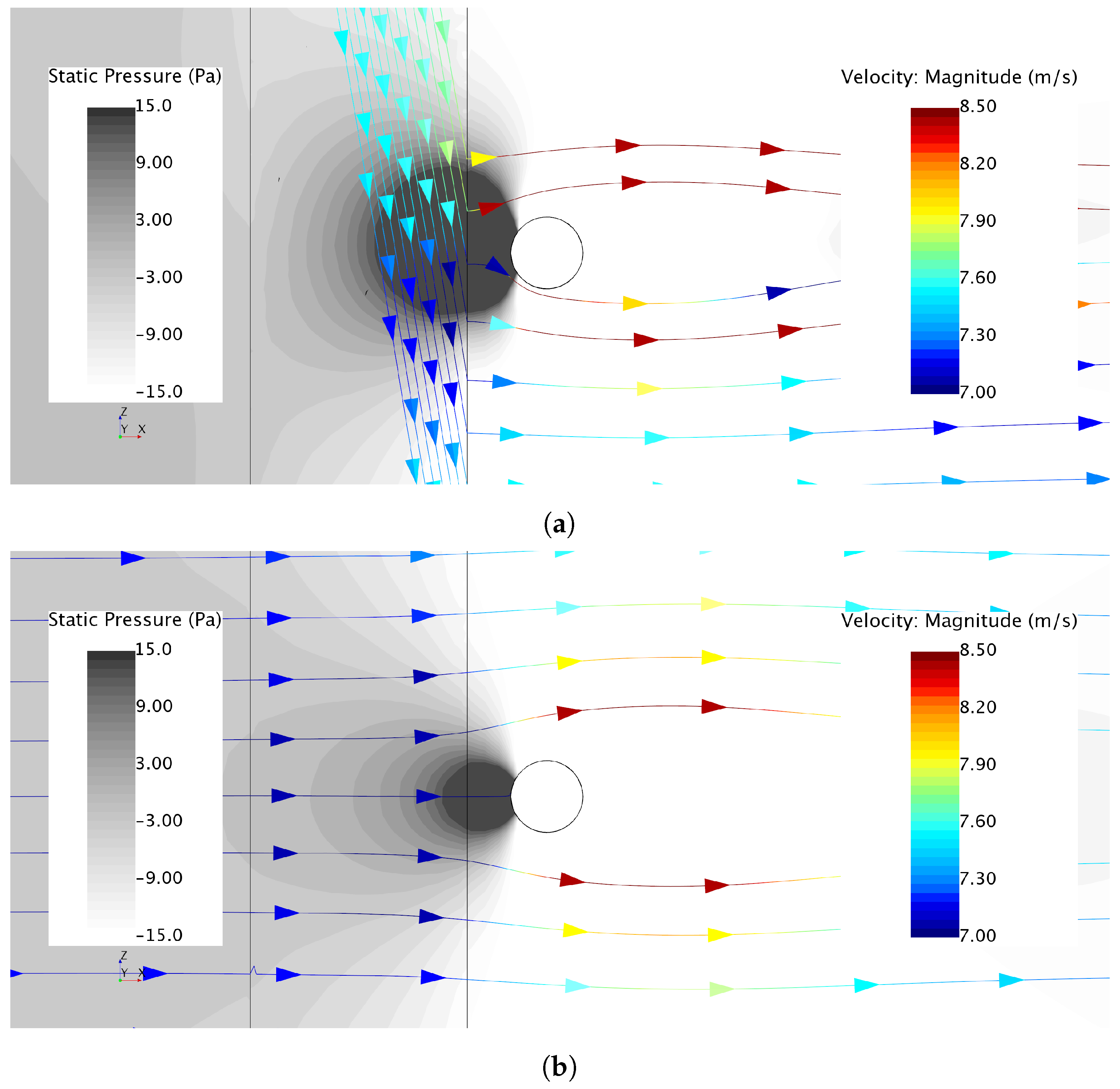
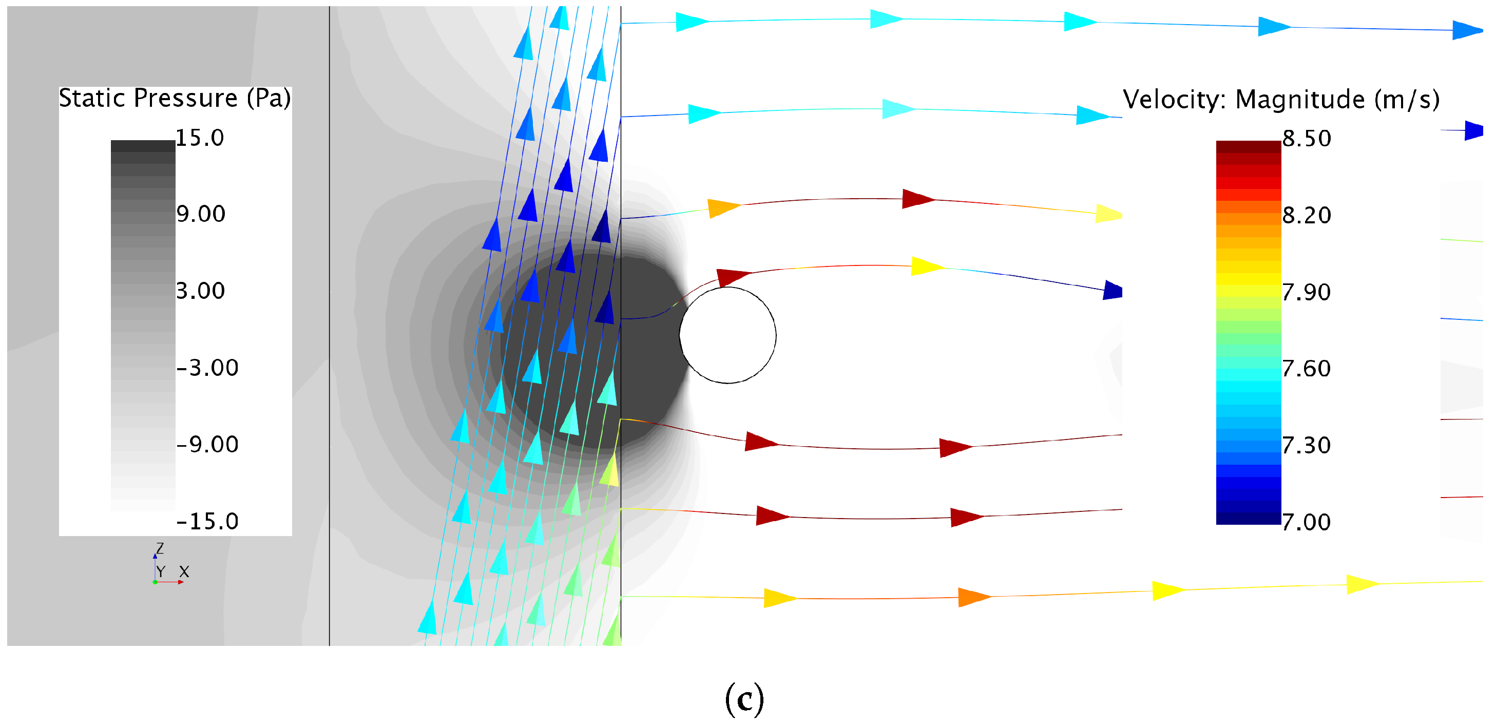
Figure 9. Even though it was placed downstream, and hence the wake did not travel through the MRF region, there is a minor effect on the upstream region. This can be related to how the static pressure field interacts with the flow inside the MRF. In
Figure 10 three longitudinal cuts through the flow field are shown: one to the left (
Figure 10a,
m), one in the middle (
Figure 10b,
m) and one to the right (
Figure 10c,
m), as seen from the upstream direction. In each of the figures the static pressure field is shown together with the streamlines of the relative velocity projected on the respective plane and coloured by their velocity magnitude. While the streamlines do not show any unusual behaviour, the magnitude of the velocity does. It can be observed that the pressure field created by the presence of the cylinder reaches into the MRF domain and causes the flow to decelerate. Therefore, the flow that passed through this high pressure zone exited the MRF domain with a considerable lower velocity magnitude than the flow that exits the MRF zone before passing the cylinder. This causes the imbalance that can be observed in
Figure 9.
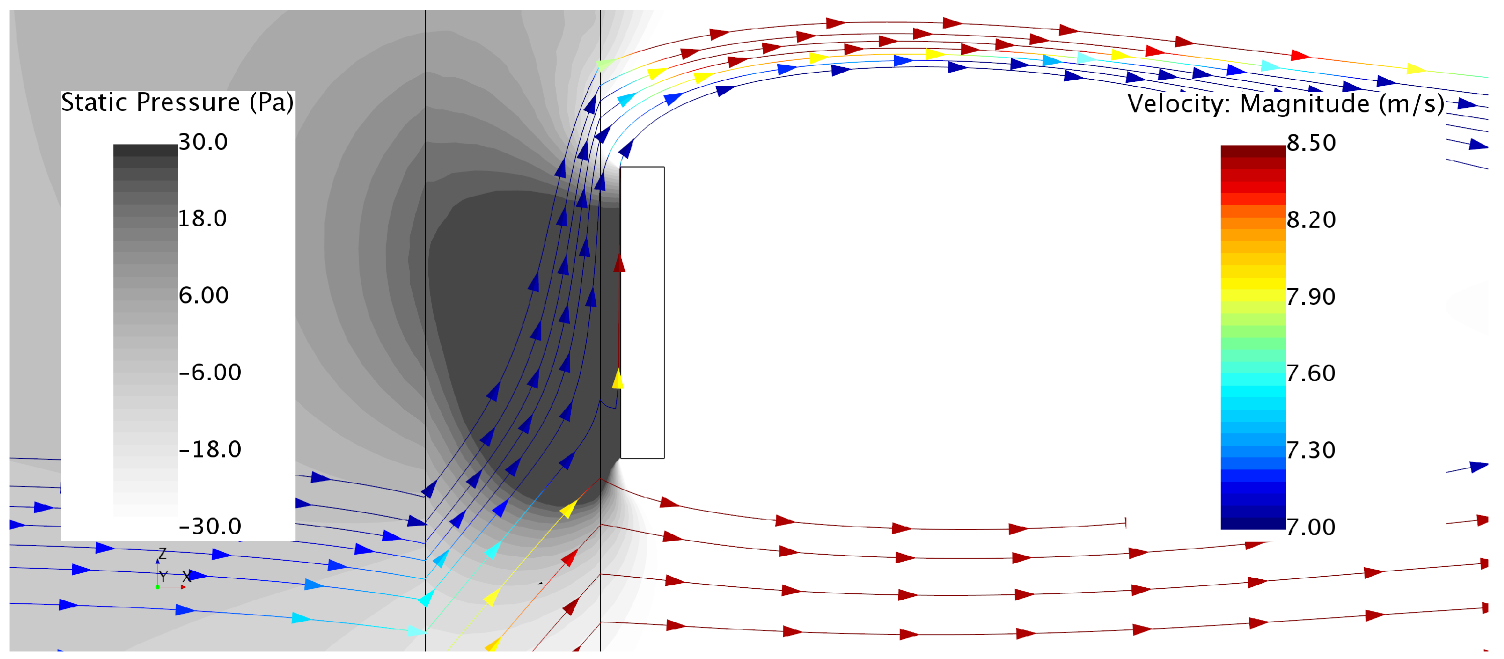
3.2.3. Case F3—Box (Downstream)
Finally, a square box was placed downstream of the MRF region. This object was of particular interest, since a similar set-up, previously studied in [
19], showed a significant interference effect on the flow field around it. From the results presented in
Figure 11, it can be observed that an object of this size had a notable effect on the upstream region, all the way to
m. In the case without blades, a large non-uniformity in the velocity distribution can be observed. As in case F2 (downstream cylinder), this deviation is caused by the built up in static pressure (
Figure 12), which causes the streamlines in the MRF region to decelerate. Therefore, higher velocities were observed in the lower and right hand side compared to the upper and left hand side of the box (
Figure 11).
4. Discussion
The results presented in the previous section clearly show the non-physical behaviour of the MRF approach. It was shown that flow properties coming from the upstream region are within the MRF domain transported with the streamlines of the relative velocity instead of the streamlines of the absolute velocity. This is reasonable, given that the streamlines of the absolute velocity often collide with the frozen rotor geometry in the MRF approach, and the streamlines of the relative velocity travel around the blades. Therefore, information would be lost by using absolute streamlines for the transport of properties. However, this can cause problems in the downstream region, especially in the case of large temperature variations. In extreme cases, such as those presented for the extended MRF zone (Case T2), the temperature field can be rotated by , meaning that regions that should experience not more than ambient conditions in reality are now heated considerably and vice versa. It shall be stressed that this behaviour is not an issue of the specific commercial solver used in this study, but can be observed in other solvers as well. The issue arises from transferring the equations from a stationary to a rotating reference frame and back without compensation for field properties, which should be invariant to the transformation in reference frame, such as the temperature.
Possible work-arounds for this problem could be the following. Since the degree of rotation is proportional to the length of the MRF domain, one possibility is to adjust the MRF length so that the field rotates . This has, however, the disadvantage that the domain could considerably grow in size. This would not be practical for the main cooling fan of a car, since the underhood environment is very narrow and the MRF domain must not intersect with any non-rotational-symmetric stationary parts. Another possibility is to map the temperature field at the upstream MRF interface to the downstream interface. By doing so, the distortion of the temperature field through the MRF region would not affect the field downstream of the fan and more accurate results could be obtained.
Regarding the effect from different geometrical structures placed up- and downstream of the MRF interfaces, various influences could be observed. If the structure is located in front of the upstream interface, the wake will be transported in the same way as the temperature field, i.e., by means of the streamlines of the relative velocity. However, the effect on the downstream flow field is far less than for the temperature field, since the wake of the blades is dominating the flow field downstream of the fan. If the obstacle is located downstream of the MRF region, another effect can be observed. The structures close to the downstream interface induce an increase in static pressure. If the increased static pressure field reaches into the MRF domain, it causes the streamlines in the rotating reference frame to decelerate, yielding a distorted flow field. It was found that amount of distortion is dependent on the size of the obstacle and its distance to the downstream interface. In the case of the downstream cylinder, the effect is relatively small, especially when including the fan blades. If the size of the obstacle is considerably larger, as for the box (case F3), the static pressure field will induce a distortion in the flow field that is prominent in both cases, with and without fan blades. Using the MRF approach in combination with a mixing-plane interface at the downstream interface of the region can improve the flow field predictions substantially. However, it eliminates most of the temperature information, as this approach averages all properties in the tangential direction.
5. Conclusions
In this study, the possibilities and limitations of the multiple reference frame method in predicting relevant features of the flow field were investigated for an axial cooling fan. Special focus was given to the transport of a non-uniform temperature field over the MRF region, and the effect different objects being placed up- and downstream of the MRF domain have on the flow field.
The study showed that both the temperature field and wake structures originating in the upstream region are transported by the streamlines of the relative velocity in the MRF domain. Therefore, those fields are rotated by an angle that is dependent on the length of the MRF zone, the presence of blades and the relation between the axial velocity and the rotation rate of the fan. It is found that the angle of rotation for the temperature and the flow field are the same for a given set-up. The presence of the fan blades also plays a role in the degree of rotation, which could be seen by the fact that the temperature and flow field have a higher degree of rotation when there is no blade geometry present in the MRF zone compared to the case with blades.
To summarize, users of the MRF approach for the simulation of axial cooling fans and other applications where temperatures are involved, are advised to be cautious. If the heat source upstream of the MRF domain is uniformly distributed over the cross-section of the fan, the effect from using an MRF approach should be minimal. However, when a notable non-uniformity in the temperature field is present, an RBM simulation should be performed instead. For the flow field it is found that obstructions located upstream of the fan only cause minor effects in the flow field downstream of the fan, since the wake of the fan blades is dominant. Large structures, such as a control box located downstream of the fan, are found to cause major disturbances in the upstream flow field. This is due to the increase in static pressure upstream of the obstacle, which can reach into the MRF domain, depending on the size and distance from the MRF interface. The pressure field itself is not affected by the rotating reference frame, but it causes the streamlines in the moving reference frame to decelerate and hence causes a non-uniformity which can be perceived as a rotation. In the narrow underhood environment around the cooling fan this makes an accurate prediction of the flow and temperature conditions very difficult. The MRF method is therefore not recommended for such applications.
Author Contributions
Conceptualization, R.F. and T.B.; methodology, R.F. and T.B.; validation, R.F.; formal analysis, R.F.; investigation, R.F.; data curation, R.F.; writing—original draft preparation, R.F.; writing—review and editing, R.F., S.S., T.B., E.W.; visualization, R.F.; supervision, S.S., E.W., A.B. and T.B.; project administration, A.B.; funding acquisition, A.B.
Funding
This research was funded by the Swedish Energy Agency under the grant number 42096-1 and the Volvo Car Corporation.
Acknowledgments
The authors would like to thank the Swedish National Infrastructure for Computing (SNIC) for providing computational resources for the simulations.
Conflicts of Interest
The authors declare no conflict of interest. The funders had no role in the design of the study; in the collection, analyses, or interpretation of data; in the writing of the manuscript, or in the decision to publish the results.
Abbreviations
The following abbreviations are used in this manuscript:
| CFD | Computational Fluid Dynamics |
| IDDES | Improved Delayed Detached Eddy Simulation |
| LES | Large Eddy Simulation |
| LF | Lumped Fan (Model) |
| MRF | Multiple Reference Frame |
| RANS | Reynolds-Averaged Navier Stokes |
| RBM | Rigid Body Motion |
| SGS | Sub-Grid Scale |
| SST | Shear Stress Transport |
References
- Shankaran, G.V.; Dogruoz, M.B. Validation of an advanced fan model with multiple reference frame approach. In Proceedings of the 2010 12th IEEE Intersociety Conference on Thermal and Thermomechanical Phenomena in Electronic Systems, ITherm 2010, Las Vegas, NV, USA, 2–5 June 2010; pp. 1–9. [Google Scholar] [CrossRef]
- Dogruoz, M.B.; Shankaran, G. Computations with the multiple reference frame technique: Flow and temperature fields downstream of an axial fan. Numer. Heat Transf. Part A Appl. 2017, 71, 488–510. [Google Scholar] [CrossRef]
- Lien, S.T.J.; Ahmed, N.A. Numerical simulation of rooftop ventilator flow. Build. Environ. 2010, 45, 1808–1815. [Google Scholar] [CrossRef]
- Zhao, L.; Chen, W.; Liu, S.; Zhang, H.; Liu, J.; Gao, Y.; Arens, E. Experimental and numerical investigations of indoor air movement distribution with an office ceiling fan. Build. Environ. 2017, 130, 14–26. [Google Scholar] [CrossRef]
- Liu, S.H.; Huang, R.F.; Lin, C.A. Computational and experimental investigations of performance curve of an axial flow fan using downstream flow resistance method. Exp. Therm. Fluid Sci. 2010, 34, 827–837. [Google Scholar] [CrossRef]
- Liu, J.; Lin, H.; Purimitla, S.R. Wake field studies of tidal current turbines with different numerical methods. Ocean Eng. 2016, 117, 383–397. [Google Scholar] [CrossRef]
- Hobeika, T.; Sebben, S. CFD investigation on wheel rotation modelling. J. Wind. Eng. Ind. Aerodyn. 2018. [Google Scholar] [CrossRef]
- Gullberg, P.; Löfdahl, L.; Adelman, S.; Nilsson, P. A Correction Method for Stationary Fan CFD MRF Models. SAE Tech. Pap. Ser. 2009, 1. [Google Scholar] [CrossRef]
- Gullberg, P.; Löfdahl, L.; Adelman, S.; Nilsson, P. An Investigation and Correction Method of Stationary Fan CFD MRF Simulations. SAE Tech. Pap. Ser. 2009, 1. [Google Scholar] [CrossRef]
- Kobayashi, Y.; Kohri, I. Study of Influence of MRF Method on the Prediction of the Engine Cooling Fan Performance. SAE Tech. Pap. 2011. [Google Scholar] [CrossRef]
- Kohri, I.; Kobayashi, Y. Prediction of the Performance of the Engine Cooling Fan with CFD Simulation. SAE Int. J. Passeng. Cars Mech. Syst. 2010, 3, 508–522. [Google Scholar] [CrossRef]
- Gullberg, P.; Löfdahl, L.; Nilsson, P.; Adelman, S. Continued Study of the Error and Consistency of Fan CFD MRF Models. SAE Tech. Pap. Ser. 2010, 1. [Google Scholar] [CrossRef]
- Gullberg, P.; Löfdahl, L.; Nilsson, P. Cooling Airflow System Modeling in CFD Using Assumption of Stationary Flow. SAE Tech. Pap. Ser. 2011, 1. [Google Scholar] [CrossRef]
- Kobayashi, Y.; Yoshida, K.; Nagano, H.; Kohri, I. Proper Orthogonal Decomposition Analysis of Flow Structures Generated around Engine Cooling Fan. SAE Int. J. Passeng. Cars Mech. Syst. 2014, 7, 728–738. [Google Scholar] [CrossRef]
- Peng, W.; Li, G.; Geng, J.; Yan, W. A strategy for the partition of MRF zones in axial fan simulation. Int. J. Vent. 2019, 18, 64–78. [Google Scholar] [CrossRef]
- Lim, S.M.; Dahlkild, A.; Mihaescu, M. Aerothermodynamics and exergy analysis of a turbocharger radial turbine integrated with exhaust manifold. In Proceedings of the 13th International Conference on Turbochargers and Turbocharging, London, UK, 16–17 May 2018. [Google Scholar]
- Siemens. Simcenter StarCCM+ Documentation; Siemens Product Lifecycle Management Software, Inc.: Plano, TX, USA, 2019. [Google Scholar]
- Zhai, Z.J.; Zhang, Z.; Zhang, W.; Chen, Q.Y.; Zhai, Z.J.; Chen, Q.Y. Evaluation of Various Turbulence Models in Predicting Airflow and Turbulence in Enclosed Environments by CFD: Part 1—Summary of Prevalent Turbulence Models Evaluation of Various Turbulence Models in Predicting Airflow and Turbulence in Enclosed Environ. HVAC&R Res. 2007, 13, 853–870. [Google Scholar]
- Franzke, R.; Sebben, S. Validation of Different Fan Modelling Techniques in Computational Fluid Dynamics. In Proceedings of the 21st Australasian Fluid Mechanics Conference, Adelaide, Australia, 10–13 December 2018. [Google Scholar]
© 2019 by the authors. Licensee MDPI, Basel, Switzerland. This article is an open access article distributed under the terms and conditions of the Creative Commons Attribution (CC BY) license (http://creativecommons.org/licenses/by/4.0/).


