Abstract
The Emissions Trading System in the European Union was introduced to achieve the climate goal of reducing emissions by around 43% between 1990 and 2030. Accordingly, the costs of emission allowances are part of power generation and, by extension, the price of electricity. Theoretical works thus suggest a positive relationship between the price of emission allowances and electricity. However, this has not been validated empirically for phase III of the Emissions Trading System in the short run as part of the price setting mechanism of electricity producers. Our evidence suggests an opposite effect: According to our empricial results, both European Power Exchange (EPEX) day-ahead and intraday markets are negatively affected during phase III. We further test for a potentially asymmetric influence with the help of quantile regressions. Altogether, the outcome has implications for policy-makers and calls for further attention by academics and policy-makers in the future design of the Emissions Trading System, especially under larger amount of renewables in the electricity system.
1. Introduction
The European Union introduced the first and largest trading system for greenhouse gases in the world, the Emissions Trading System (EU ETS). Its launch in 2005 came as a direct consequence of the Kyoto Protocol as a means of achieving the climate objective of reducing emissions by 43% between 1990 and 2030 [1]. The design is based on a cap and trade system, which allows only a fixed amount of emissions for various greenhouse gases such as carbon dioxide (CO), nitrous oxide (NO), and perfluorocarbons (PFCs). In the past, the annual limit of greenhouse gases has been decreased in order to reduce greenhouse gases and to thus achieve climate goals.
The actual design of the cap and trade system represents a challenging task for policy-makers. On the one hand, the price for emission allowances needs to be fairly high in order to provide an incentive to reduce emissions [2]. On the other hand, the price should not threaten economic development. Therefore, policy-makers need to combine social, economic, and environmental considerations. For example, the European Commission has broadened the number of industries that are subject to the trade mechanism as part of the modifications when transitioning from phase II to III of the Emissions Trading System. Nowadays, about 11,000 heavy energy-using installations are part of the EU ETS, accounting for approximately 45% of all emissions in Europe. In particular, the entire power production sector in Germany is obligated to participate in the EU ETS. Accordingly, every power company must hold a sufficient number of European Emission Allowances (EUA) by the end of the year, whereby each EUA entitles the energy producer to emit one ton of carbon dioxide or its equivalents.
Since 2013, phase III of the EU ETS represents the status quo. It differs from phase II (years 2008–2012) in the following key dimensions [1]:
- Reduction of free allocation. Most notably, policy-makers reduced the free allocation of emission allowances once again. This has led to 40% of allowances being sold at auction. For instance, the entire power production sector is forced to buy allowances at auction. As such, electricity producers must buy emission allowances on the energy exchange when they have exceeded their allowance, e.g., due to higher-than-expected emissions. Additionally, in the period of 2014–2016, they reduced the number of certificates by 900 million. These certificates will be used as a market stability reverse mechanism to match demand and supply.
- Expansion to more industries and further greenhouse gases. The EU ETS now accounts for additional greenhouse gases that were not part of phase II, such as nitrous oxide (NO) and perfluorocarbons (PFCs). In addition, it adds a wider array of industry sectors, such as manufacturing industries and aircraft operators.
- EU registry. While national registries collected the names of companies qualified for emissions trading during phase II, these were replaced in phase III by a registry encompassing the full European Union, which now includes 31 countries participating in the EU ETS. The European registry was introduced in order to establish a better control mechanism throughout the member states.
Based on the changes between phase II and III of the ETS, one would expect a stronger influence of the carbon price on electricity prices. In theory, the necessary expenditures on emission allowances should increase costs for operators of power plants and it is thus likely to be linked to the price of electricity. For example, lignite-fired power plants emit about 0.984 tons of carbon dioxide per 1 MWh energy, while power plants fired by natural gas produce about 0.548 tons of carbon dioxide per 1 MWh energy. (Retrieved from http://www.eia.gov/tools/faqs/faq.cfm?id=74&t=11 on 11 June 2019.) In other words, one can assume an influence of emission allowances on electricity prices if the underlying pass-through rate is nonzero [3,4]. Consequently, the price of EUA is incorporated in the price setting algorithms of electricity producers, thus resulting in electricity price fluctuations in the short run [5]. Policy-makers demand such evaluations, which allow them to assess whether emissions trading encourages high amounts of sustainable sources of electricity generation on a national or international scale.
Our literature survey later reveals that the link between carbon and European Power Exchange (EPEX) electricity prices has been studied for phase II of the EU ETS but not for phase III. Here, we follow earlier research which has focused on the short-run relationship between EUA prices and electricity prices as a means to study the price setting mechanisms of electricity firms (e.g., References [5,6]). It is thus the key contribution of this paper to quantify the impact of carbon prices on EPEX electricity prices during phase III of the EU ETS. For this purpose, we specifically compare the effect across day-ahead and intraday markets. We additionally calculate the distributional properties of the pass-through rate by means of quantile regression to test whether a price premium for EUA is only added for a certain threshold price.
Our results suggest a negative relationship between emission allowances and electricity prices. The corresponding implications are discussed by considering the intentions of policy-makers when designing phase III of the EU ETS. Especially, the findings are later set in relation to the context of various proposed changes to the EU ETS that are currently under consideration by policy-makers. Altogether, these insights can help to improve the future market design for emissions trading in order to achieve the desired climate objectives. Our findings should be seen as a starting point for future research as they call for further attention to better understand the consequences for price setting that result from the introduction of the EU ETS.
2. Related Work
This section reviews related works concerning the influence of carbon prices on the price of electricity.
2.1. Long Run vs. Short Run Relationship
Previous works have analyzed the relationship between carbon prices and the price of electricity as part of an empirical study. These reveal statistical evidence of such a relationship across several markets in both the long and short run yet not for phase III of the EU ETS.
In regard to the long run, Bunn and Fezzi [7] find a positive relationship between the carbon price and the price of electricity in the U. K. during phase I of the EU ETS. Their analysis reveals that a 1% change in the carbon price results in an increase in electricity prices by % in the equilibrium case. In the short run, this study observes a visible shock in electricity prices after a few days. A similar, positive relationship in the long run is observed in the Spanish market [8,9]. However, the effect here is of a lesser magnitude; i.e., a 1% change in the carbon price yields a % increase in the long run during phase II and in the first year of the third phase [9]. In addition, the findings suggest a smaller impact for a lower carbon price than for a higher one.
On the other hand, there is also strong evidence in favor of a short-run relationship. For example, in the Nordic electricity market, the price of EUA tends to considerably influence the electricity price in the short run [10,11]. Cotton and Mello [5] examined the Australian approach to reducing greenhouse gas emissions. The authors found no impact in the long run but did in the short run. Analogously, our analysis is concerned foremost with the short-run relationship, since we not only investigate the day-ahead market but also the price setting mechanism in the intraday market, where empirical evidence is especially limited.
According to Bannoer et al. [12], the relatively small impact may result from the almost constant carbon price, at least during the period from 2010 until 2013, and conclude, therefore, that the carbon price has only a very small effect. However, this work only studies phase II and cannot assess whether the additional adjustments from phase III have been effective.
2.2. Asymmetric Pass-Through Rate
The ratio of costs passed on to customers has been extensively discussed in the literature. From a theoretical point of view, this pass-through rate should account for 100% in perfect markets [3]. However, the condition of perfect markets seldom holds in reality, thus resulting in a lower pass-through rate [4]. The pass-through rate depends on additional factors, such as the energy mix, the demand, as well as the supply of energy [13]. In addition, recent works [14,15] find a less than 100% but asymmetric pass-through of costs in the German market. In particular, a pass-through rate of at least 84%, ranging from 98% to 104%, is found for different load periods [14]. As a consequence, increasing the carbon price is supposed to influence the electricity price more strongly than decreasing carbon prices. As a result, the price setting mechanism might be only affected by carbon prices exceeding a certain price threshold. In Section 4.3, we control for this effect by utilizing quantile regressions in order to compute the distributional properties of the carbon effect on electricity prices.
2.3. Directional Influence
Previous research reports contradictory evidence regarding the direction of the influence. Jouvet and Solier [4] revealed significant positive as well as negative effects of EUA prices in each year from 2005 through 2011 (except 2009) for all European markets, with the negative impact mostly occurring in the Italian market. For the German and Austrian electricity markets, the effects are not consistent. Furthermore, Aatola et al. [16] found a positive but asymmetric influence of the carbon price on European electricity prices—such as U. K., France, Netherlands, Germany, Spain, and the Nordic countries. However, in the short run, they did not find a clear pattern. A work by Woo et al. [17] also points to a strong regional dependency of the emission price effect. The author’s found a short-run price effect between dollar and dollar in Western USA with respect to a 1 dollar carbon price change.
The unclear patterns regarding the direction of the influence remain in different phases of the EU ETS, revealing mixed effects. Phase II evinces a significant positive effect of the carbon price on the hourly electricity price in the short run [6]. Paraschiv et al. [18] estimate a state space model with time-varying coefficients between 2010 and 2012 to correct the variance, finding both a positive and negative influence of the EUA price on the day-ahead electricity price. However, none of the above papers has focused on the EPEX electricity prices of both the intraday and day-ahead auction market or, on top of that, studied the changes in the relationship between EU ETS phases II and III. One of the reasons is that the introduction of phase III occurred only recently and, therefore, empirical evidence relating to it is still scarce. As a remedy, this paper examines the impact of carbon prices in phases II and III on German and Austrian day-ahead and intraday electricity prices.
3. Methods and Materials
In the following, we present our autoregressive model, as well as the underlying dataset. Additional materials and robustness checks can be found in the Supplementary Materials.
3.1. Modeling of Electricity Prices
Electricity entails several unique characteristics that differentiate it from other commodities, such as the need to instantaneously match the electricity demand and supply, the diverse array of electricity sources, as well as the lack of available storage capability. As a result, electricity prices are highly volatile and driven by seasonality [19,20,21,22], which makes the modeling of electricity prices challenging. In this respect, recent literature has yielded two dominant approaches to modeling electricity prices. First, co-integration models such as vector autoregressive (VAR) and vector error correction (VEC) models (e.g., References [6,8,9,23]). These are especially suited to research questions that seek to investigate interdependencies between multiple variables. For example, one can use them to quantify the impact of load on electricity prices and vice versa. Second, autoregressive models and their variants (e.g., with a moving-average term) are commonly used when studying the impact of several covariates on a single price variable (e.g., References [21,24,25,26]). For this reason, we follow the latter approach by modeling electricity prices as an autoregressive process. Specifically, we define one model for each hour, since we therefore can better capture the daily fluctuation of electricity prices [27]. This is beneficial as it allows us to focus on the short-run relationship and thus the price setting of electricity producers, i.e., how EUA is actually incorporated by decision-makers. This is also motivated by earlier research that concentrated on the short-run relationship when studying the pricing power of EUA [5,6].
Besides the choice of the model, we need to carefully consider the inclusion of covariates since a variety of exogenous factors might influence electricity prices. Common examples are fuel prices (e.g., References [10,18,28,29]), power generation (e.g., References [8,30]), feed-ins from renewables (e.g., References [8,9,31,32,33,34]), and economic factors (e.g., Reference [8]). Given the broad spectrum of considered covariates, there seems to be no consistent recommendation as to which variables to insert, especially as the significance of the impact varies from study to study. We thus follow a two-pronged approach, which first chooses the control factors that are most common in the previous literature, namely, load (as a proxy for power demand) and solar/wind power generation [29]. Moreover, we additionally use a set of additional covariates (coal price, gas price, oil price, and foreign exchange rate) as part of a robustness check.
3.2. Autoregressive Time Series Model
We now present the method by which we empirically measure the impact of EUA on electricity prices. For this purpose, we follow previous research and use autoregressive models with exogenous variables (ARX). We specifically estimate separate models for each hour of the day [18,27]. This introduces additional degrees of freedom that can reflect, e.g., differences in the electricity mix between peak and off-peak hours. Our online appendix lists robustness checks with additional covariates and a global model with de-seasonalization [35], resulting in similar findings.
Our key independent variable of interest is given by the price for EUA. We additionally incorporate the infeeds of wind farms and photovoltaic power plants, as well as the grid load, since they serve as standard control variables when studying electricity prices [22,23]. These also cover most factors that are specific to the demand and supply sides. In case of the latter, the short-term dynamics of prices are mostly affected not by power generation from fossil fuels but by variable sources of power generation, of which wind and solar power represent the largest shares in the German market. Moreover, we incorporate dummy variables for the weekday and the month in order to adjust for seasonal variations.
3.3. Asymmetric Influence Via Quantile Regressions
Previous research argues in favor of a nonlinear pass-through of emission costs [15]. Accordingly, the influence on electricity prices is stronger at the upper end of the merit order curve conditional on a large infeed from expensive sources of power generation. The influence of carbon prices on electricity prices is thus likely to be asymmetric [9,36]. For instance, we expect a large effect when all power plants produce electricity, since this might include carbon-intensive forms of power generation. As a consequence, increasing the carbon price is supposed to impact the electricity price more strongly than decreasing carbon prices. This suggests that the coefficient is subject to variations and thus attains values that are dependent on the electricity price. In other words, the estimated free parameters of each quantile regression cover the quantiles of the distribution of electricity prices. Therefore, our later analysis also addresses the distributional influence of carbon prices on electricity prices.
For this purpose, we use quantile regressions, which differ from ordinary least squares (OLS). Whereas the latter measures the impact of predictor variables on the mean of an outcome variable, quantile regressions incorporate the entire distribution of electricity prices by estimating the influence of carbon prices at different percentiles of the dataset [37]. Therefore, we can shed light upon potential variations in the effect across different percentiles.
Mathematically, the OLS regression estimates global coefficients that quantify the effect of regressors X on the electricity price at the mean. This is given by . Quantile regression, by contrast, allows us to estimate the effect of predictor variables X on a selected quantile of outcome variable [37]. Hence, we obtain separate coefficients for different quantiles of , given by . This thus yields the full impact of carbon prices across the full (conditional) distribution of electricity prices. For mathematical details of this estimation procedure, we refer to Reference [37].
3.4. Dataset
An overview of our dependent variables and the covariates is presented in Table 1. The dependent variable is given by the electricity prices in the day-ahead, as well as intraday spot market. Here, delivery of electricity for a certain hour h of day d can be traded continuously from 3 p.m. on day until 30 min before hour h on day d. Hence, we follow previous research and perform our analysis based on the average hourly price [29]. The prices originate from the European Power Exchange (EPEX), which is a joint venture of the Energy Exchange (EEX) and the French Powernext.

Table 1.
Overview of variables taken into account in the subsequent evaluation.
Here, our main variable of interest is the price of European Emission Allowance (EUA). Table 2 reports the descriptive statistics. As part of the switch from phase II to III in the EU ETS, the price of EUA has undergone major changes. As such, the mean price per EUA dropped by % from €11.61 to €5.23. Furthermore, the standard deviation declined by from 3.56 to 1.02.
Table 2.
Descriptive statistics for the price of European Emission Allowance (in €) in phases II and III.
4. Results
This section analyzes the influence of the carbon prices on electricity prices. We first test the stationarity of our time series and, afterwards, estimate the autoregressive models and the quantile regressions for the hours .
4.1. Stationarity
We need to validate whether our time series are stationary in order to rule out a spurious regression [35]. Here, the augmented Dickey–Fuller (ADF) tests find stationary time series in levels for both electricity prices, the load, as well as for feed-ins from solar and wind power for each hour separately. The hourly EUA price is stationary in levels during phase II and phase III but not over the entire period. Therefore, in order to obtain stationary time series, we take the first differences of EUA when studying the entire sample. Due to the extensive nature of the ADF test for each hour and covariates (504 ADF tests), the values are omitted for brevity.
4.2. Influence of Carbon Price during the EU ETS Regimes
We now estimate the impact of the EUA price on both day-ahead and intraday electricity prices. Section 4.1 has already established that the price of EUA is integrated of order one during the entire sample. Therefore, we instead consider the first differences in order to ensure the absence of a spurious regression [35]. Detailed results are reported in the online appendix, while we restrict our presentation to key findings in the following.
We perform a series of diagnostic tests: First, we find only stationary residuals and thus eliminate the risk of analyzing a spurious regression. Second, the p-value belonging to the F-statistics of each model is zero and, thus, the combination of model variables has an influence on the dependent variable. Furthermore, we find autocorrelation of the residuals by using the Durbin–Watson test, while a Breusch–Pagan test reveals heteroscedastic residuals. To adjust the test values for both autocorrelation and heteroscedasticity, we use the Newey–West procedure (e.g., Reference [35,38]). Its advantage is that we yield t-statistics that are robust to a general form of serial correlation and heteroscedasticity but let the regression coefficients be unaffected [35].
According to Table 3, the influence of the EUA price on electricity prices is as follows. In the day-ahead market, the coefficient of the EUA time series (in the form of first differences) is non-significant at common statistical significance levels for each hour of the day (Table 3 exemplary reports the hours 8, 16, and 24). These findings change when we split the dataset into phase II and III. While in phase II, the EUA price has an impact in hours 13 to 16, in phase III the EUA price has an significant negative impact in each hour of the day, even in nighttime. Controversially, the impact remains negative over the entire day. We observe a quite similar picture with regard to the intraday market. In this case, the price of emission allowances shows a negative impact in phase III, being highly significant.
Table 3.
Estimated coefficients of separate autoregressive models belonging to different hours () of the day: These measure the influence of the EUA price on electricity prices of the EU ETS. Dependent variables are the hourly day-ahead and intraday electricity prices.
The relative impact on the dependent variable subsequent to a one standard deviation increase in the EUA price enables us to compare the strength of the effect independent of the scaling and thus across both the day-ahead and intraday markets. In the day-ahead market, the corresponding coefficient is negative ranging from −0.32 to −0.13. This means that a one standard deviation increase in the price of EUA results in a −0.32 to −0.13 standard deviation decrease in the electricity price variable depending on the hour of the day. In the intraday market, the significant negative impact lies between −0.36 to −0.28, revealing that the intraday market is more strongly affected by EUA prices.
Consistent with previous literature, we find that demand- and supply-side factors show a statistically significant impact on electricity prices, though the results differ across markets. In the day-ahead market, the impact of solar and wind feed-ins on the price of electricity is weaker than in the intraday market. Additionally, load governs the intraday market to a larger extent. Several other studies discuss the influence of external variables, such as load and feed-ins from renewables, in more detail (cf. References [23,29,33,39]).
According to the goodness-of-fit, all models in the day-ahead market as well as in the intraday market reveal a strong explanatory power with an adjusted above 0.94.
Robustness Checks
As part of our robustness checks, we estimate an analysis in accordance to Wolff and Feuerriegel [29] by incorporating additional control variables in order to ensure that their inclusion does not confound our results. These variables concern the daily coal price (Credit Suisse Commodity Benchmark for coal API 2 spot return price index at the Amsterdam-Rotterdam-Antwerp Hub in USD/t.) , the gas price (Setting price of natural gas first near future at the virtual gas trading hub Title Transfer Facility (TTF) in EUR/MWh.) , the oil price (Brent crude oil spot price in USD per barrel.) , and the closing price of the USD-EUR exchange rate . We again take the first differences where time series are integrated of order one. As earlier, we only report the t-statistics that are robust to heteroscedasticity and serial correlation. The results are given in Table 4 for the impact of the EUA price on both the day-ahead and intraday electricity price.
Table 4.
Estimated coefficients of separate autoregressive models belonging to different hours () of the day as part of a robustness check: These measure the influence of the EUA price on electricity prices of the EU ETS incorporating control variables. Dependent variables are the hourly day-ahead and intraday electricity prices.
The estimation results reveal the same picture as our earlier analysis: The EUA shows a significantly negative impact in the day-ahead market during phase III. Interestingly, the EUA price positively affects the electricity price for the hour 24 when the solar feed-in is zero, while in the main model, we find a small positive impact for hour 16. In the case of the intraday market, the price of emission allowances shows a negative impact in phase III that is statistically highly significant. Hence, a one standard deviation increase in the price of EUA results in a −0.79 to −2.53 standard deviation decrease in the electricity price variable.
4.3. Asymmetric Influence of the Carbon Price on Electricity Prices
As previous research suggests [3,9,36], the carbon price may have an asymmetric impact on electricity prices. Therefore, we perform quantile regressions for the 25%, 50%, and 75% quantiles. Figure 1 and Figure 2 present the estimation results across different phases of the EU ETS.
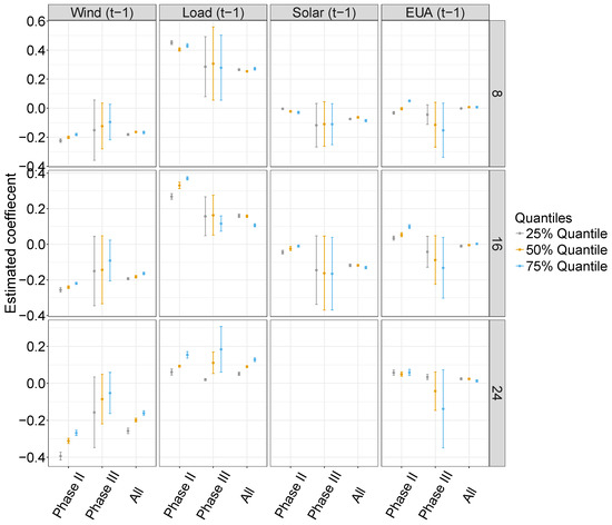
Figure 1.
Results of the quantile regression for the day-ahead electricity market indicating an asymmetric influence of the EUA price on day-ahead electricity prices: Here, separate regressions are analyzed belonging to different hours (); see different rows. We first obtained difference EUA prices for the entire period to ensure stationary time series.
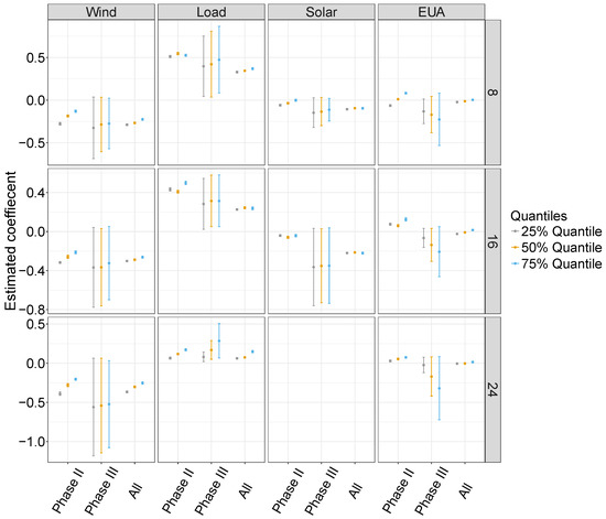
Figure 2.
Results of the quantile regression for the intraday electricity market indicating an asymmetric influence of the EUA price on intraday electricity prices: Here, separate regressions are analyzed belonging to different hours (); see different rows.
Interestingly, we observe different results for the day-ahead and intraday markets compared to the results from Section 4.2. First of all, we find that the impact of the price of EUA on electricity prices appears predominantly in phase III of the EU ETS. However, we see a considerable impact in the day-ahead market in phase III, with a diverging influence for the 25% and 75% quantiles. In the 25% quantile, a one standard deviation increase in the price of EUA results in an low impact with values around zero. By contrast, in the 75% quantile, the price of EUA links to a decrease by up to −0.165 standard deviations in the day-ahead electricity price for hour 8. In the intraday market, the relationship remains stronger with statistically significant standardized coefficients up to 0.320 in the 75% quantile for hour 24. All in all, our results indicate an asymmetric influence of the EUA price.
5. Discussion of Findings
This section discusses our findings regarding the relationship between carbon and electricity prices. Our abovementioned findings from the autoregressive models deserve attention. According to expectation, the price of electricity is supposed to rise with a higher carbon price, thus giving rise to a positive relationship, since spending on emission allowances introduces an additional cost driver. We thus shed light on the potential reasons for the nature of the relationship:
- Excess supply of emission allowances. Since we find a weak and inconsistent influence of the emission allowance prices on the electricity price, the price must be too low to play a significant role in power generation. This is particularly evident in our autoregressive model during phase II, where we observe no direct effect. The same model evinces a statistically significant negative impact only for the day-ahead and intraday market in phase III. These findings are consistent with previous research, suggesting that the impact of low carbon prices is rather moderate [9,15] and becomes observable only above certain thresholds. Surprisingly, even though more industries are forced to engage in emissions trading in phase III of the EU ETS, actual power generation and the corresponding electricity price seem unaffected by carbon trading. Consequently, the presence of nonsignificant influences partially originate from an excess supply of emission allowances.
- Changing energy mix. The Emissions Trading System functions in a highly intricate interplay with other policies, especially the incentivized introduction of renewable energy sources. Renewables account for a growing portion of the total electricity supply. (Retrieved from http://www.bmwi-energiewende.de/EWD/Redaktion/Newsletter/2015/1/Meldung/infografik-strommix-2014-erneuerbare-auf-rekordhoch.html on 9 June 2019.) As these electricity sources replace fossil-fuel power plants, the demand for emission allowances (relative to the total electricity demand) must decrease at the same pace. Otherwise, the burgeoning share of renewables inherently results in an excess supply of emission allowances, thus counteracting one of the main advantages of renewable energies.
- Merit order effect. Large carbon prices are also linked to larger marginal costs for carbon-intensive power plants as opposed to renewable energies. This explains the differential influence of carbon prices as revealed by our quantile regressions. An additional reason is given by support schemes for renewables that sometimes grant preferential treatment. That is, wind and solar power must be consumed before power is generated via other means. Hence, carbon prices have a less significant effect on electricity prices when renewables produce a high amount of electricity, i.e., when electricity prices are low.
6. Conclusions
The European Union has established a market for trading emission allowances of greenhouse gases. Its objective is to contribute to sustainability goals and to reduce emissions. The spending on emission allowances represents an integral cost driver of power generation affecting operational decision-making and thus price setting. It is therefore of interest to investigate the relationship between carbon and electricity prices across different phases of the Emissions Trading System.
6.1. Summary of the Findings
This paper contributes to the existing literature by analyzing the (asymmetric) impact of carbon prices on EPEX electricity prices, with a special focus on the intraday market. We thus use an autoregressive model with exogenous variables. The results show a behavior of the model contradictory to the intentions of policy-makers. We find a statistically highly significant negative impact in the intraday market during phase III of the European Union Emissions Trading System. Here, a one standard deviation change in the price of emission allowances decreases the price of electricity by up to −0.44 standard deviations. Moreover, the effect is weaker in the day-ahead market during phase III, while throughout phase II, we do not observe any measurable effect. Among the reasons are a growing share of renewable energy resources and an excess supply of emission allowances.
Most notably, we observe differences between the day-ahead and intraday markets. While our autoregressive model detects a weaker (negative) short-run impact of the EUA price in the day-ahead market, we find a stronger significant negative impact of the EUA price on the intraday electricity prices during phase III of the EU ETS. This outcome partially contradicts empirical studies into other markets, which mostly measure a positive impact [9]. Similarly, further research cannot find a short-run impact of the carbon prices on electricity prices [5]. Paraschiv et al. [18] provides evidence of both a positive and negative influence.
Altogether, various factors explain the relationship between emission allowances and electricity generation. Among them, we identify a combination of an excess supply of emission allowances, a growing share of renewable energy source, and the merit order effect. Since we are not aware of previous literature examining the price of emission allowances in the intraday market, we cannot compare these results to the findings of others.
To conclude, the transition from phase II to phase III of the EU ETS was motivated by policy-makers in order to reduce emissions from electricity generation. This is in correspondence to our results, according to which the price of European Emission Allowance was not linked to electricity prices at common statistical significance thresholds during phase II. It is also in line with expectations, as one was not required to hold EUA for carbon-intensive power generation during this phase. For phase III, however, we find evidence that counteracts the intention of policy-makers. Based on our model, we see that a higher EUA price is not reflected in higher electricity prices. Prior literature discussing the general design of the EU ETS has already suggested that the influence of carbon prices is fairly low, particularly due to a large supply. This is also seen in our analysis: The average price for EUA dropped extensively during the move from phase II to phase III of the EU ETS, i.e., from more than 11 €/tCO to a little more of 5 €/tCO. This eases the pressure for electricity providers to incorporate carbon prices in their pricing models and to thus adapt their generation accordingly (e.g., they could be incentivized to use existing carbon-intensive capacities for electricity generation before an increase in carbon prices takes place).
6.2. Limitations and Call for Future Research
We focused on the short-run relationship of the EUA price and electricity prices since our aim is to investigate the price setting mechanism of electricity providers in both the day-ahead and intraday market. By following a short-run view, we were able to address the intraday variation of electricity prices for each hour of the day, which corresponds to the price setting mechanisms in the markets. As a results, future studies could built upon our research and analyze the impact of EUA prices on electricity prices, focusing on the long run. This would allow a deeper understand of how EUA prices are reflected in electricity prices. While a strength of our work is the focus on the price setting decisions, another limitation of this study originates from the circumstance that, as in other research, the actual trading models of energy firms are proprietary and thus not available for research. Nevertheless, our approach by studying ex post prices is able to shed light on the underlying price setting mechanism.
Our findings deserve attention by academics and policy-makers who should critically reflect whether this matches their intention. Hence, we regard this paper as a starting point for future research in analyzing the functioning of EU ETS with respect to electricity producers. The design of appropriate markets for emissions trading can considerably benefit from further research as many questions are still left unanswered. First of all, it is worthwhile to extensively investigate interactions between different regulations in order to derive policy implications. Here, one could even consider studying distinct price setting mechanisms, especially under increased shares of renewables in the system. These might better pass-through costs of emission allowances and thus help establish real incentives to reduce greenhouse gases. Second, further effort is necessary to understand how the price and trading volume of emission allowances impacts other commodities. With the upcoming advances in the Emissions Trading System, future research should continuously monitor the effect of carbon prices on electricity prices in order to evaluate all impending policy changes.
Supplementary Materials
The following are available online at https://www.mdpi.com/1996-1073/12/15/2894/s1.
Author Contributions
Both authors contributed equally to this work.
Funding
This research received no external funding.
Conflicts of Interest
The authors declare no conflict of interest.
References
- European Commission. The EU Emissions Trading System. 2018. Available online: https://ec.europa.eu/clima/policies/ets (accessed on 29 March 2019).
- Hintermann, B.; Peterson, S.; Rickels, W. Price and Market Behavior in Phase II of the EU ETS: A Review of the Literature. Rev. Environ. Econ. Policy 2015, 10, 108–128. [Google Scholar]
- Sijm, J.; Neuhoff, K.; Chen, Y. CO2 cost pass-through and windfall profits in the power sector. Clim. Policy 2006, 6, 49–72. [Google Scholar] [CrossRef]
- Jouvet, P.A.; Solier, B. An overview of CO2 cost pass-through to electricity prices in Europe. Energy Policy 2013, 61, 1370–1376. [Google Scholar] [CrossRef]
- Cotton, D.; Mello, L.D. Econometric analysis of Australian emissions markets and electricity prices. Energy Policy 2014, 74, 475–485. [Google Scholar] [CrossRef]
- Thoenes, S. Understanding the Determinants of Electricity Prices and the Impact of the German Nuclear Moratorium in 2011. Energy J. 2014, 35, 61–78. [Google Scholar] [CrossRef]
- Bunn, D.; Fezzi, C. Interaction of European carbon trading and energy prices. J. Energy Mark. 2009, 2, 53–69. [Google Scholar] [CrossRef]
- Bello, A.; Reneses, J. Electricity price forecasting in the Spanish market using cointegration techniques. In Proceedings of the 33rd Annual International Symposium on Forecasting (ISF 2013), Seoul, Korea, 23–26 June 2013; pp. 1–7. [Google Scholar]
- Freitas, C.J.P.; da Silva, P.P. European Union emissions trading scheme impact on the Spanish electricity price during phase II and phase III implementation. Util. Policy 2015, 33, 54–62. [Google Scholar] [CrossRef]
- Fell, H. EU-ETS and Nordic electricity: A CVAR analysis. Energy J. 2010, 31, 1–25. [Google Scholar] [CrossRef]
- Jabłońska, M.; Viljainen, S.; Partanen, J.; Kauranne, T. The impact of emissions trading on electricity spot market price behavior. Int. J. Energy Sect. Manag. 2012, 6, 343–364. [Google Scholar] [CrossRef]
- Bannör, K.; Kiesel, R.; Nazarova, A.; Scherer, M. Parametric model risk and power plant valuation. Energy Econ. 2016, 59, 423–434. [Google Scholar]
- Chernyavs’ka, L.; Gullì, F. Marginal CO2 cost pass-through under imperfect competition in power markets. Ecol. Econ. 2008, 68, 408–421. [Google Scholar]
- Hintermann, B. Pass-Through of CO2 Emission Costs to Hourly Electricity Prices in Germany. J. Assoc. Environ. Resour. Econ. 2016, 3, 857–891. [Google Scholar] [CrossRef]
- Zachmann, G.; von Hirschhausen, C. First evidence of asymmetric cost pass-through of EU emissions allowances: Examining wholesale electricity prices in Germany. Econ. Lett. 2008, 99, 465–469. [Google Scholar] [CrossRef]
- Aatola, P.; Ollikainen, M.; Toppinen, A. Impact of the carbon price on the integrating European electricity market. Energy Policy 2013, 61, 1236–1251. [Google Scholar] [CrossRef]
- Woo, C.K.; Olson, A.; Chen, Y.; Moore, J.; Schlag, N.; Ong, A.; Ho, T. Does California’s CO2 price affect wholesale electricity prices in the Western U.S.A.? Energy Policy 2017, 110, 9–19. [Google Scholar] [CrossRef]
- Paraschiv, F.; Erni, D.; Pietsch, R. The impact of renewable energies on EEX day-ahead electricity prices. Energy Policy 2014, 73, 196–210. [Google Scholar] [CrossRef]
- Bierbrauer, M.; Menn, C.; Rachev, S.T.; Trück, S. Spot and derivative pricing in the EEX power market. J. Bank. Financ. 2007, 31, 3462–3485. [Google Scholar]
- Deng, S.; Oren, S.S. Electricity derivatives and risk management. Energy 2006, 31, 940–953. [Google Scholar]
- Knittel, C.R.; Roberts, M.R. An empirical examination of restructured electricity prices. Energy Econ. 2005, 27, 791–817. [Google Scholar]
- Weron, R. Modeling and Forecasting Electricity Loads and Prices: A Statistical Approach; John Wiley & Sons: Chichester, UK, 2007; Volume 403. [Google Scholar]
- Paschen, M. Dynamic analysis of the German day-ahead electricity spot market. Energy Econ. 2016, 59, 118–128. [Google Scholar]
- Contreras, J.; Espinola, R.; Nogales, F.J.; Conejo, A.J. ARIMA models to predict next-day electricity prices. IEEE Trans. Power Syst. 2003, 18, 1014–1020. [Google Scholar]
- Fuglerud, M.; Vedahl, K.E.; Fleten, S.E. Equilibrium simulation of the Nordic electricity spot price. In Proceedings of the 2012 9th International Conference on the European Energy Market, Florence, Italy, 10–12 May 2012; pp. 1–10. [Google Scholar]
- Ludwig, N.; Feuerriegel, S.; Neumann, D. Putting big data analytics to work: Feature selection for forecasting electricity prices using the LASSO and random forests. J. Decis. Syst. 2015, 24, 19–36. [Google Scholar]
- Weron, R. Electricity price forecasting: A review of the state-of-the-art with a look into the future. Int. J. Forecast. 2014, 30, 1030–1081. [Google Scholar] [CrossRef]
- Ferkingstad, E.; Løland, A.; Wilhelmsen, M. Causal modeling and inference for electricity markets. Energy Econ. 2011, 33, 404–412. [Google Scholar]
- Wolff, G.; Feuerriegel, S. Short-term dynamics of day-ahead and intraday electricity prices. Int. J. Energy Sect. Manag. 2017, 11, 557–573. [Google Scholar]
- Beran, P.; Pape, C.; Weber, C. Modelling German electricity wholesale spot prices with a parsimonious fundamental model—Validation and application. Util. Policy 2019, 58, 27–39. [Google Scholar] [CrossRef]
- Benhmad, F.; Percebois, J. Photovoltaic and wind power feed-in impact on electricity prices: The case of Germany. Energy Policy 2018, 119, 317–326. [Google Scholar] [CrossRef]
- Clò, S.; Cataldi, A.; Zoppoli, P. The merit-order effect in the Italian power market: The impact of solar and wind generation on national wholesale electricity prices. Energy Policy 2015, 77, 79–88. [Google Scholar]
- Gelabert, L.; Labandeira, X.; Linares, P. An ex-post analysis of the effect of renewables and cogeneration on Spanish electricity prices. Energy Econ. 2011, 33, 59–65. [Google Scholar]
- Mosquera-López, S.; Nursimulu, A. Drivers of electricity price dynamics: Comparative analysis of spot and futures markets. Energy Policy 2019, 126, 76–87. [Google Scholar] [CrossRef]
- Wooldridge, J. Introductory Econometrics: A Modern Approach, 5th ed.; Cengage Learning: Boston, MA, USA, 2012. [Google Scholar]
- Paraschiv, F.; Bunn, D.W.; Westgaard, S. Estimation and Application of Fully Parametric Multifactor Quantile Regression with Dynamic Coefficients; University of St. Gallen, School of Finance Research Paper No. 2016/07; 2016; Available online: https://ssrn.com/abstract=2741692 (accessed on 29 March 2019).
- Koenker, R.; Bassett, G. Regression Quantiles. Econometrica 1978, 46, 33–50. [Google Scholar]
- Pape, C.; Hagemann, S.; Weber, C. Are fundamentals enough? Explaining price variations in the German day-ahead and intraday power market. Energy Econ. 2016, 54, 376–387. [Google Scholar] [CrossRef]
- Würzburg, K.; Labandeira, X.; Linares, P. Renewable generation and electricity prices: Taking stock and new evidence for Germany and Austria. Energy Econ. 2013, 40, 159–171. [Google Scholar]
© 2019 by the authors. Licensee MDPI, Basel, Switzerland. This article is an open access article distributed under the terms and conditions of the Creative Commons Attribution (CC BY) license (http://creativecommons.org/licenses/by/4.0/).