Solar Irradiance Forecasts by Mesoscale Numerical Weather Prediction Models with Different Horizontal Resolutions

 , ,
, ,
Abstract
:1. Introduction
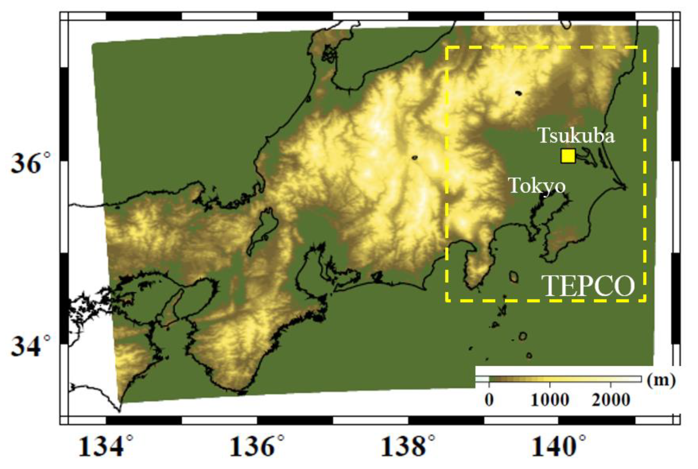
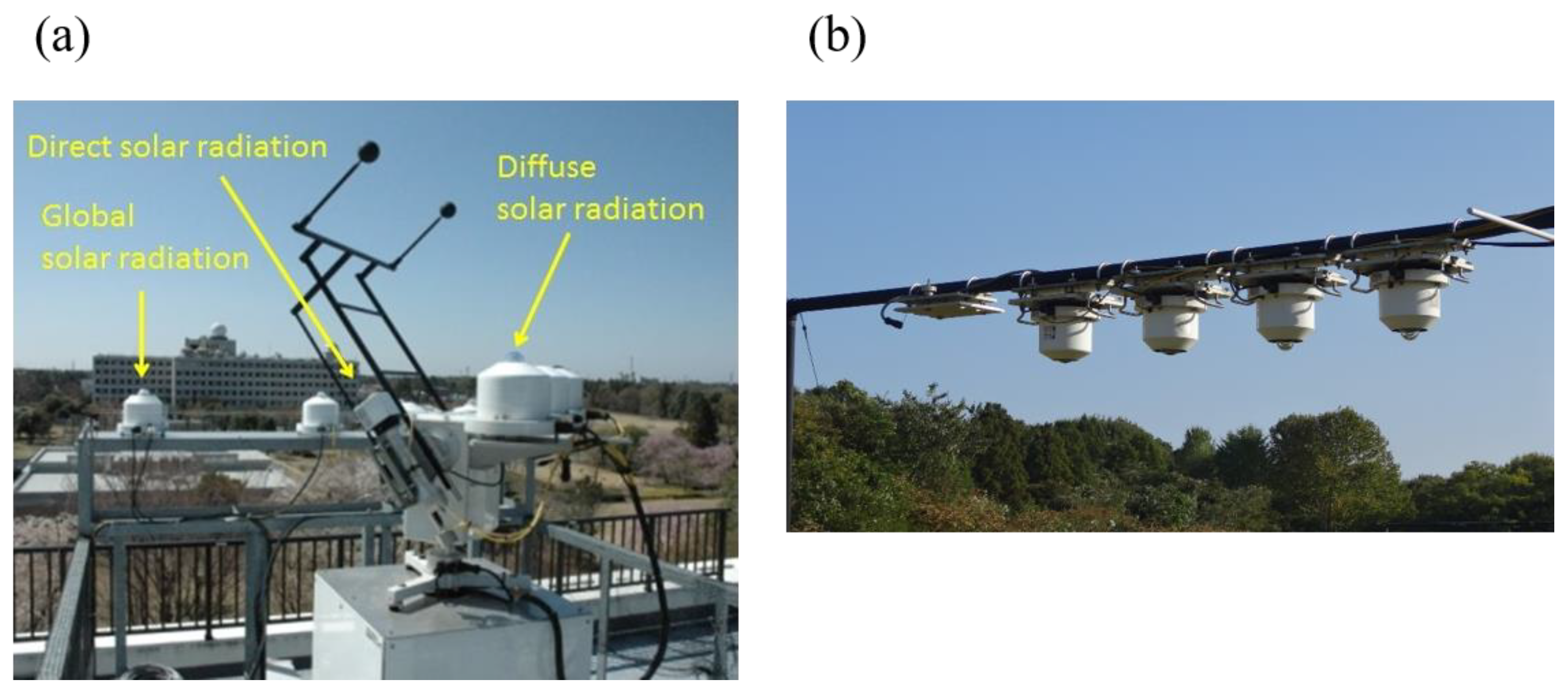
2. Observation data
2.1. Global Solar Irradiance Data
2.2. Satellite-Derived Solar Irradiance
3. Numerical simulations
3.1. Model
3.2. Performance Metrics
4. Validation results
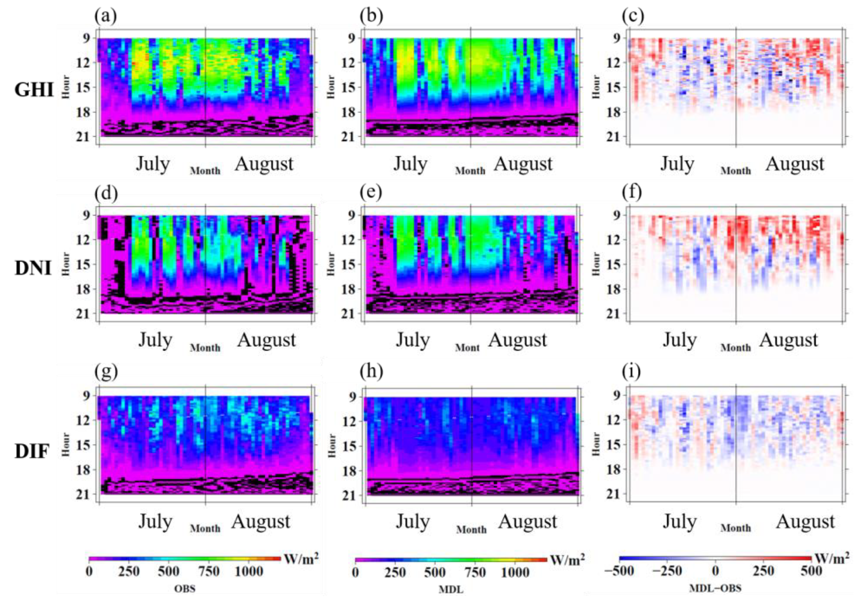
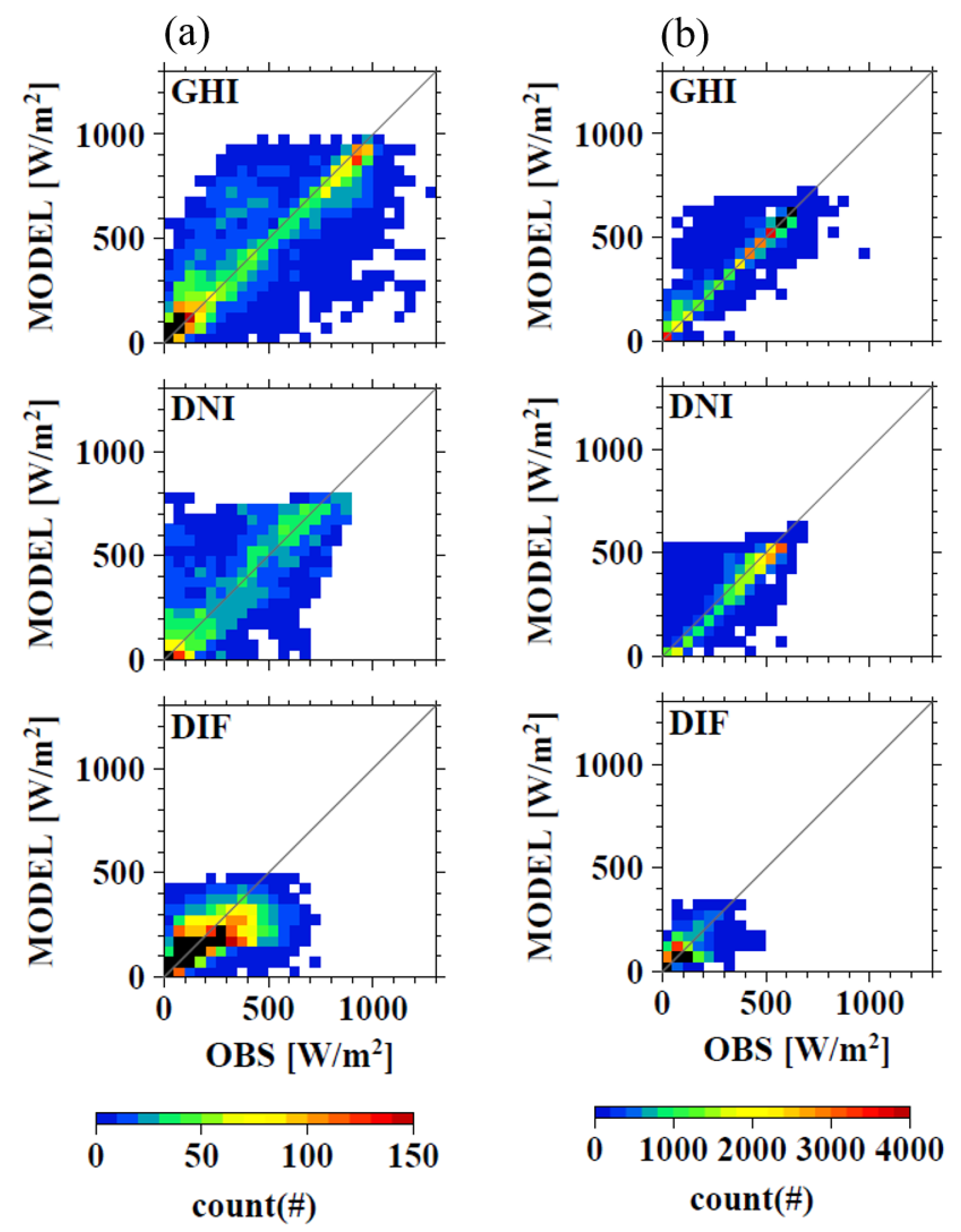
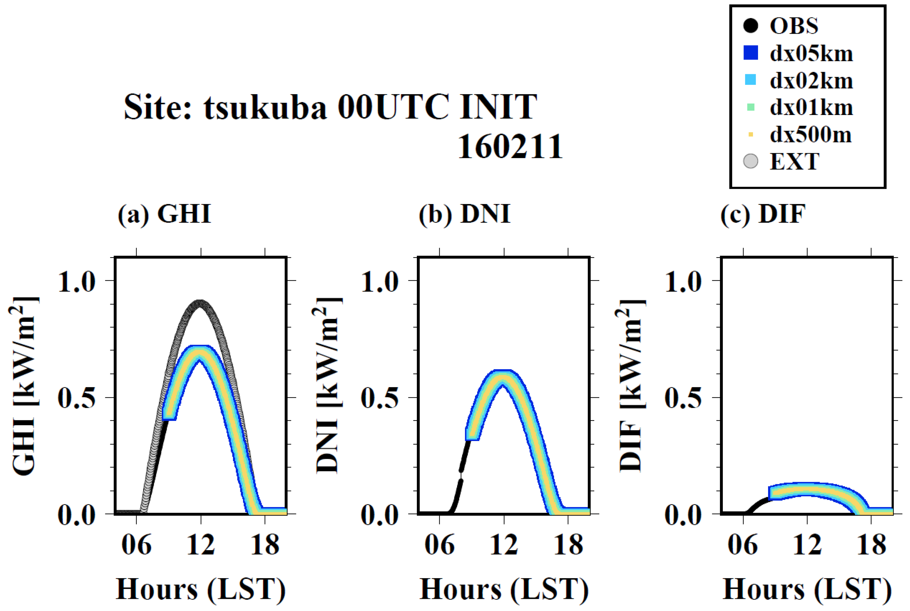
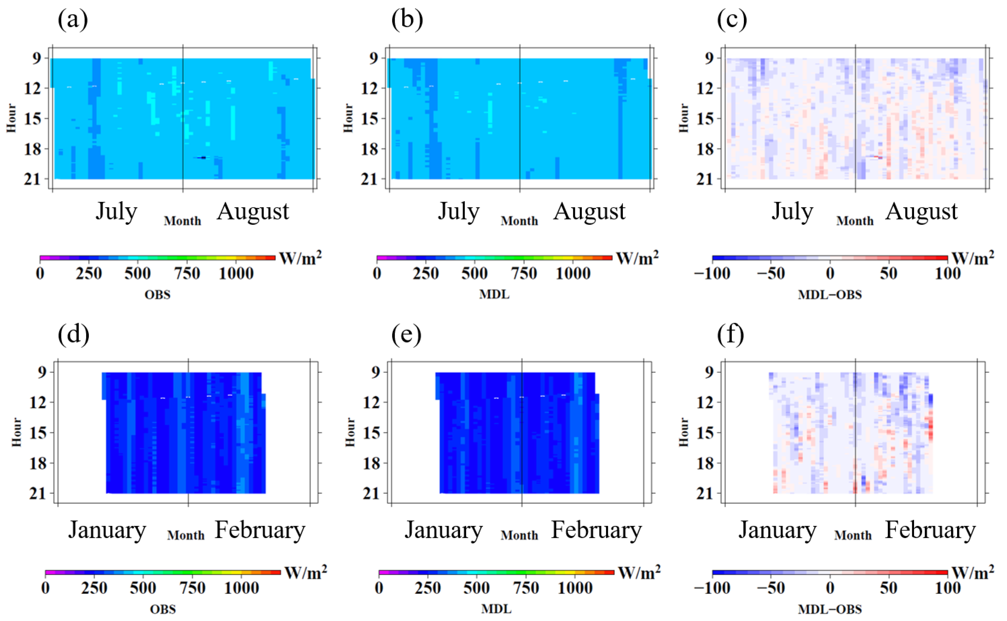
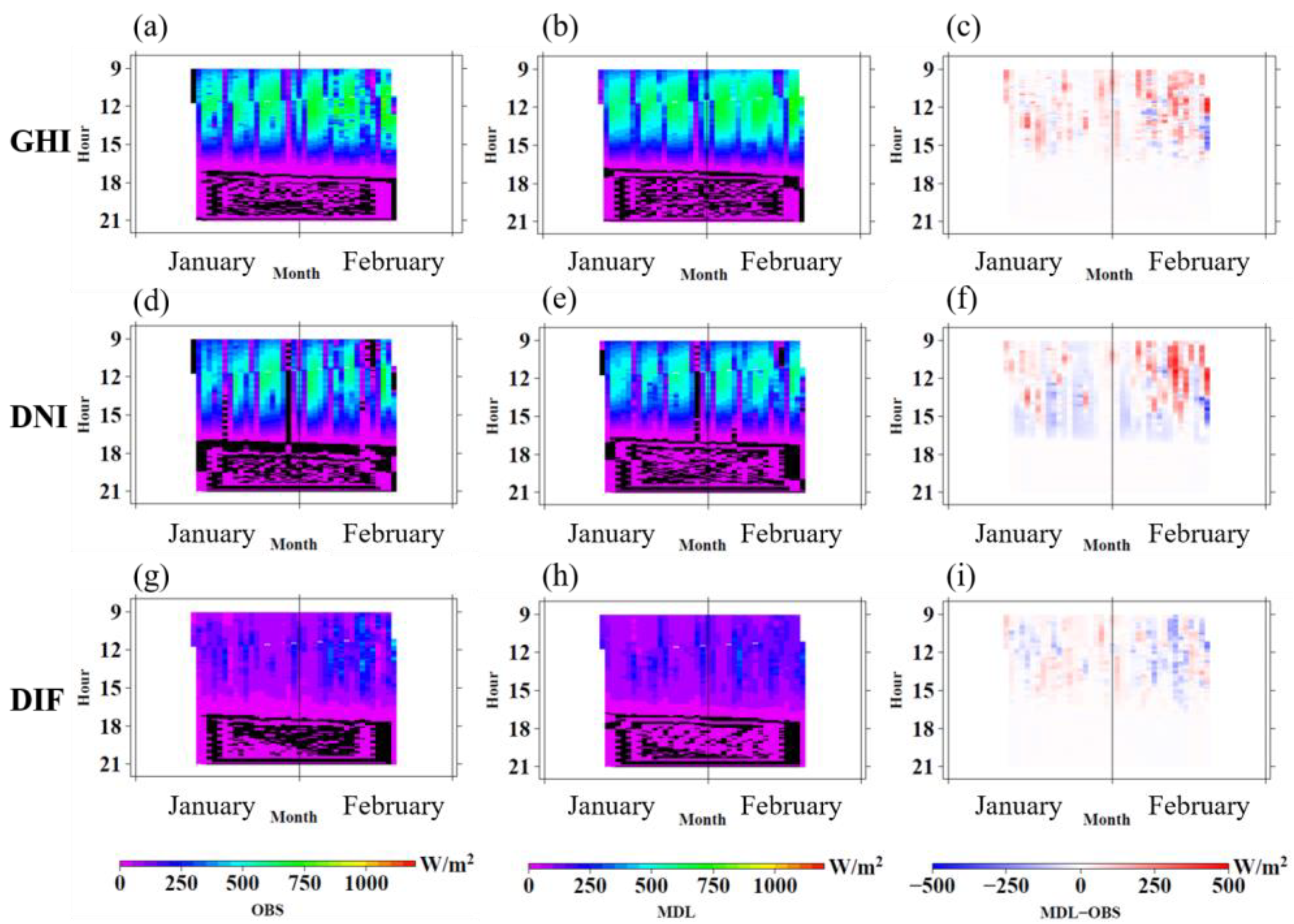
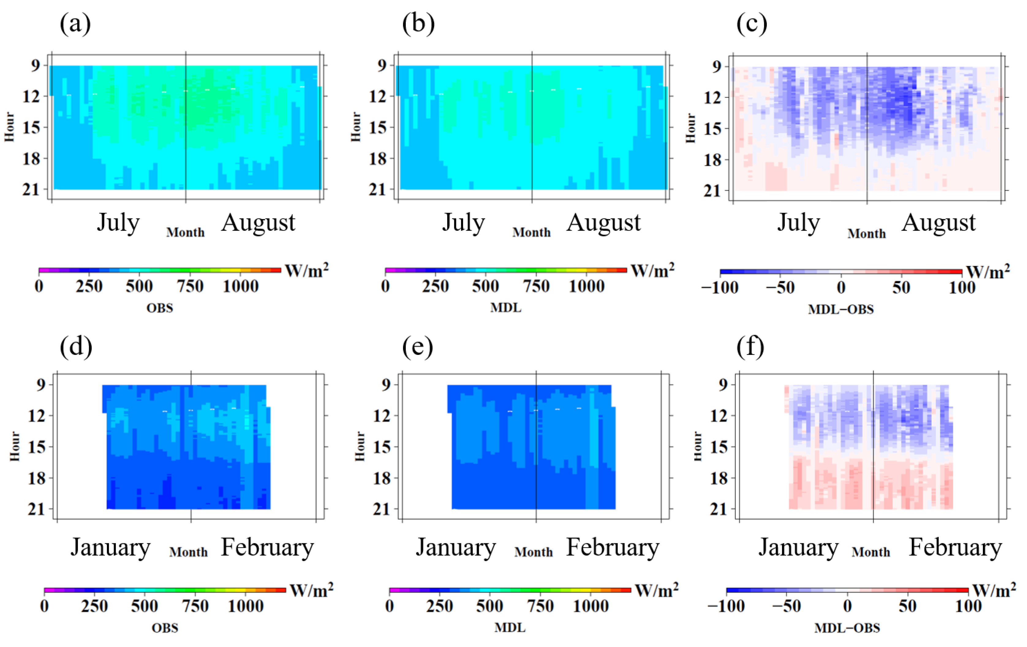
4.1. Validation of GHI, DNI and DIF
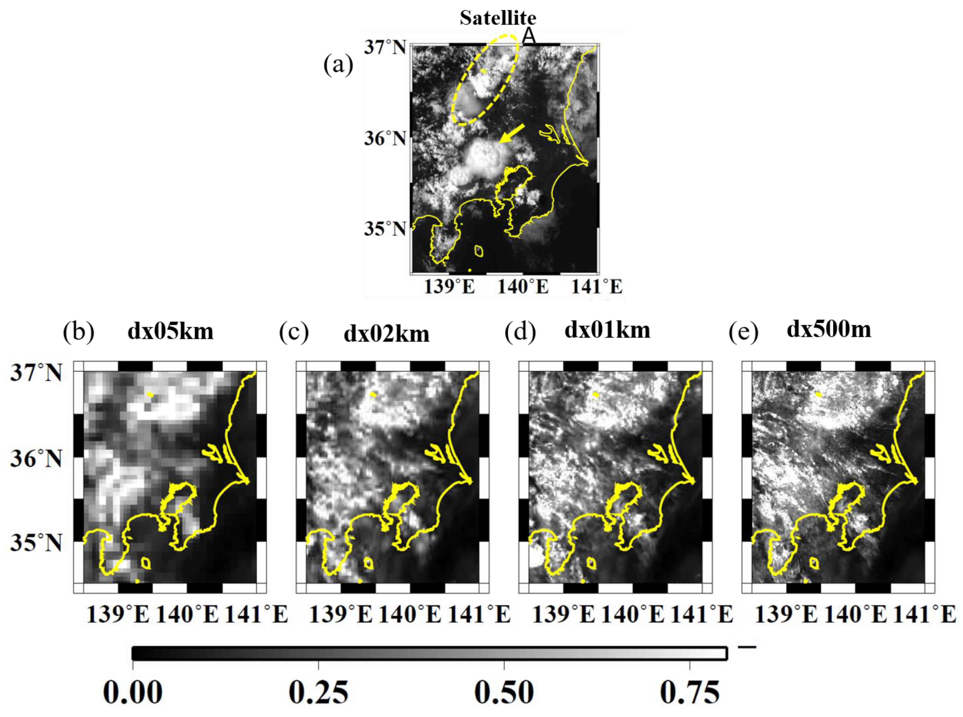
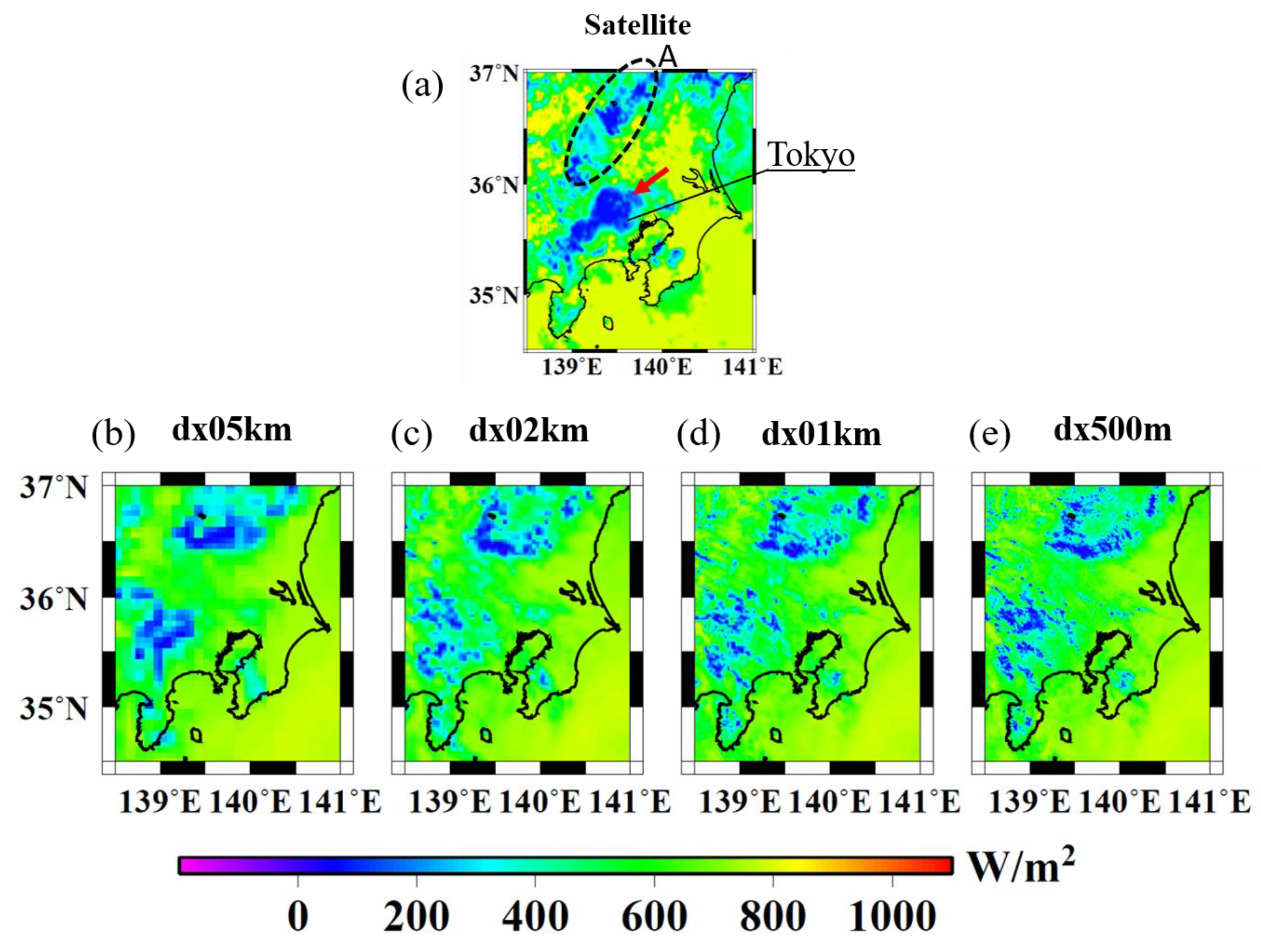
4.2. A Case Study of Cumulus Cloud Simulation
4.3. Longwave Radiation
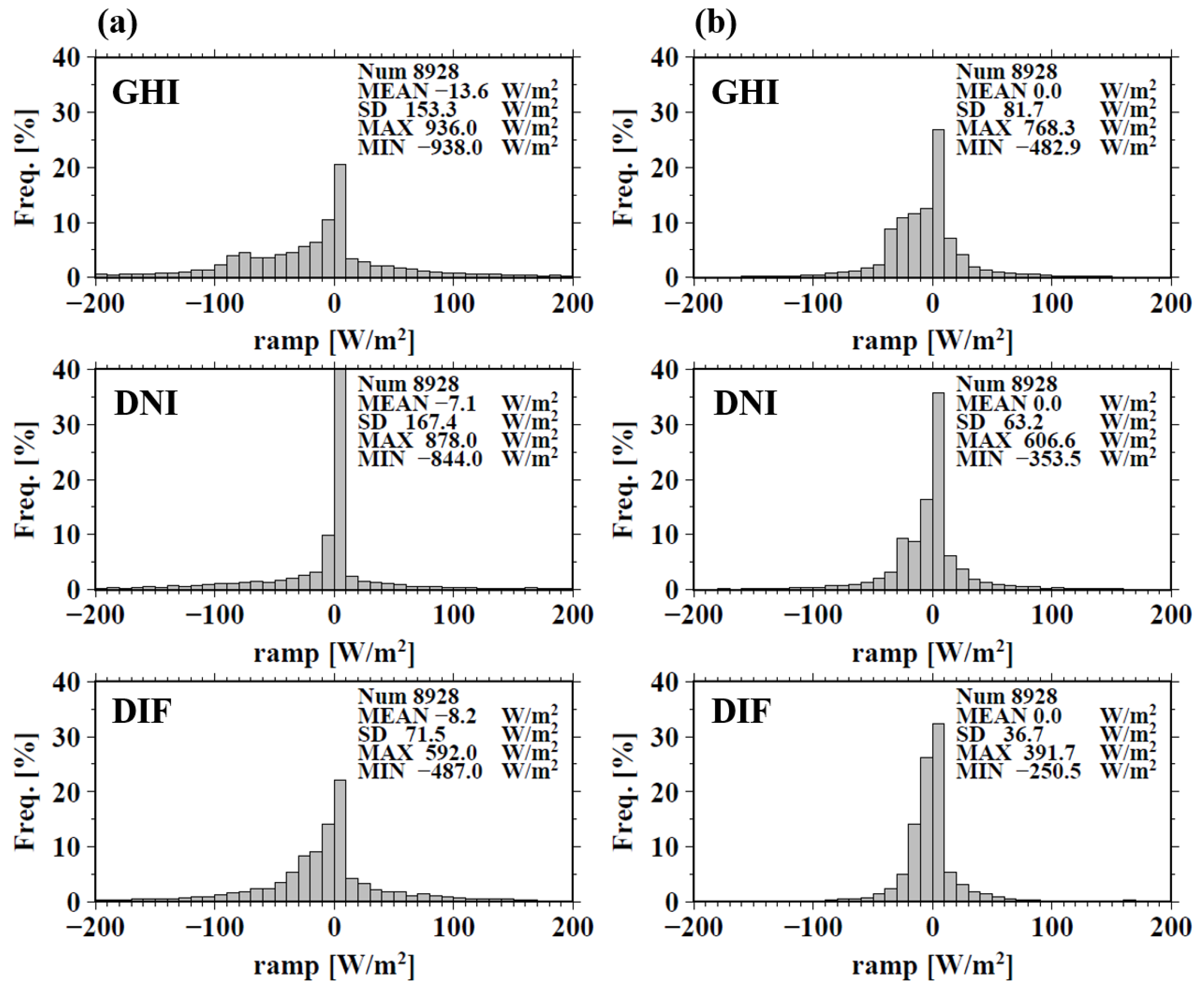
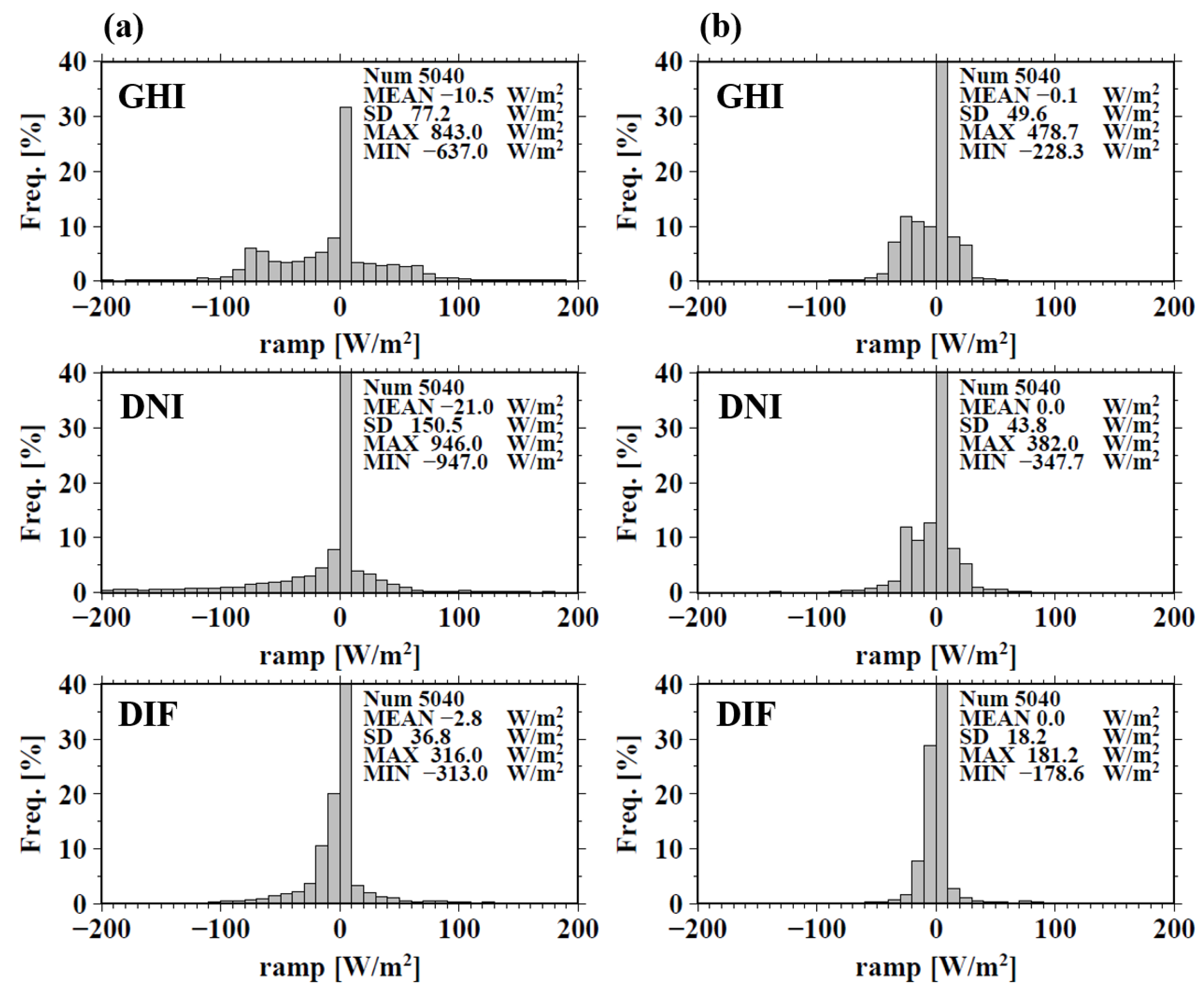
5. Ramp rate of solar irradiance
6. Summary
Author Contributions
Funding
Acknowledgments
Conflicts of Interest
References
- Schiermeier, Q. And Now for the Energy Forecast. Germany Works to Predict Wind and Solar Power Generation. Nature.com, 2016. Available online: http://www.nature.com/polopoly_fs/1.20251!/menu/main/topColumns/topLeftColumn/pdf/535212a.pdf (accessed on 6 March 2019).
- Ohtake, H.; Shimose, K.-I.; Fonseca, J.G.S., Jr.; Takashima, T.; Oozeki, T.; Yamada, Y. Accuracy of the solar irradiance forecasts of the Japan Meteorological Agency mesoscale model for the Kanto region, Japan. Sol. Energy 2013, 98, 138–152. [Google Scholar] [CrossRef]
- Ohtake, H.; Shimose, K.-I.; Fonseca, J.G.S., Jr.; Takashima, T.; Oozeki, T.; Yamada, T. Regional and seasonal characteristics of global horizontal irradiance forecasts obtained from the Japan Meteorological Agency mesoscale model. Sol. Energy 2015, 116, 83–99. [Google Scholar] [CrossRef]
- Mathiesen, P.; Kleissl, J. Evaluation of numerical weather prediction for intra-day solar forecasting in the continental United States. Sol. Energy 2011, 85, 967–977. [Google Scholar] [CrossRef]
- Perez, R.; Lorenz, E.; Pelland, S.; Beauharnois, M.; Knowe, G.V.; Hemker, K., Jr.; Heinemann, D.; Remund, J.; Müller, S.C.; Traunmüller, W.; et al. Comparison of numerical weather prediction solar irradiance forecasts in the US, Canada and Europe. Sol. Energy 2013, 94, 305–326. [Google Scholar] [CrossRef]
- Lorenz, E.; Kuhnert, J.; Heinemann, D.; Nielsen, K.P.; Remund, J.; Muller, S.C. Comparison of global horizontal irradiance forecasts based on numerical weather prediction models with different spatio-temporal resolutions. Prog. Photovolt. Res. Appl. 2016, 1626–1640. [Google Scholar] [CrossRef]
- Gregory, P.A.; Rikus, L.J. Validation of the bureau of meteorology’s global, diffuse, and direct solar exposure forecasts using the ACCESS numerical weather prediction systems. J. Appl. Meteorol. Climatol. 2016, 55, 595–619. [Google Scholar] [CrossRef]
- Sosa-Tinoco, I.; Peralta-Jaramillo, J.; Otero-Casal, C.; Lopez-Aguera, A.; Miguez-Macho, G.; Rodriguez-Cabo, I. Validation of a global horizontal irradiation assessment from a numerical weather prediction model in the south of Sonora-Mexico. Renew. Energy 2016, 90, 105–113. [Google Scholar] [CrossRef]
- Charabi, Y.; Gastli, A.; Al-Yahyai, S. Production of solar radiation bankable datasets from high-resolution solar irradiance derived with dynamical downscaling Numerical Weather prediction model. Energy Rep. 2016, 2, 67–73. [Google Scholar] [CrossRef]
- Mathiesen, P.; Collier, C.; Kleissl, J. A high-resolution, cloud-assimilating numerical weather prediction model for solar irradiance forecasting. Sol. Energy 2013, 92, 47–61. [Google Scholar] [CrossRef]
- Lin, W.; Zhang, M.; Wu, J. Simulation of low clouds from the CAM and the regional WRF with multiple nested resolutions. Geophys. Res. Lett. 2009, 36, L08813. [Google Scholar] [CrossRef]
- Ito, J.; Hayashi, S.; Hashimoto, A.; Ohtake, H.; Uno, F.; Yoshimura, H.; Kato, T.; Yamada, Y. Stalled improvement in a numerical weather prediction model as horizontal resolution increases to the sub-kilometer scale. SOLA 2017, 13, 151–156. [Google Scholar] [CrossRef]
- Wellby, S.J.; Engerer, N.A. Categorizing the meteorological origins of critical ramp events in collective photovoltaic array output. J. Appl. Meteorol. Clim. 2016, 55, 1323–1344. [Google Scholar] [CrossRef]
- Gilgen, H.; Whitlock, C.; Koch, F.; Muller, G.; Ohmura, A.; Steiger, D.; Wheeler, R. Technical Plan for BSRN (Baseline Surface Radiation Network) Data Management (Version 2.1, Final); World Radiation Monitoring Center Tech. Rep. 1, WMO/TD No. 443, World Climate Research Programme; WMO, 1995; 57p, Available online: https://library.wmo.int/index.php?lvl=notice_display&id=11762#.XKv-kJj7Q1I (accessed on 9 April 2019).
- Ohmura, A.; Dutton, E.G.; Forgan, B.; Fröhlich, C.; Gilgen, H.; Hegner, H.; Heimo, A.; König-Langlo, G.; McArthur, B.; Müller, G.; et al. Baseline Surface Radiation Network (BSRN/WCRP): New precision radiometry for climate research. Bull. Am. Meteorol. Soc. 1998, 79, 2115–2136. [Google Scholar] [CrossRef]
- McArthur, L.B.J. Baseline Surface Radiation Network (BSRN) Operation Manual (Version 1.0); WMO/TD-No. 879, World Climate Research Programme; WMO, 1998; 155p, Available online: https://library.wmo.int/index.php?lvl=notice_display&id=11769#.XKxPKSARXIV (accessed on 9 April 2019).
- The Web Site of Baseline Surface Radiation Network (BSRN). Available online: http://www.bsrn.awi.de/ (accessed on 6 March 2019).
- The Web Site of Meteorological Satellite Center. Available online: http://www.jma-net.go.jp/msc/en/ (accessed on 6 March 2019).
- Bessho, K.; Date, K.; Hayashi, M.; Ikeda, A.; Imai, T.; Inoue, H.; Kumagai, Y.; Miyakawa, T.; Murata, H.; Ohno, T.; et al. An introduction to Himawari-8/9—Japan’s New-Generation Geostationary Meteorological Satellites. J. Meteorol. Soc. Jpn. 2016, 94, 151–183. [Google Scholar] [CrossRef]
- Takenaka, H.; Nakajima, T.Y.; Higurashi, A.; Higuchi, A.; Takamura, T.; Pinker, R.T.; Nakajima, T. Estimation of solar radiation using a neural network based on radiative transfer. J. Geophys. Res. 2011, 116, D8. [Google Scholar] [CrossRef]
- Nakajima, T.Y.; Nakajima, T. Wide-area determination of cloud microphysical properties from NOAA AVHRR measurements for FIRE and ASTEX regions. J. Atmos. Sci. 1995, 52, 4043–4059. [Google Scholar] [CrossRef]
- Kawamoto, K.; Nakajima, T.; Nakajima, T.Y. A global determination of cloud microphysics with AVHRR remote sensing. J. Clim. 2001, 14, 2054–2068. [Google Scholar] [CrossRef]
- Solar Radiation Consortium 2015. Available online: http://amaterass.org/product.html (accessed on 6 March 2019). (In Japanese).
- Damiani, A.; Irie, H.; Horio, T.; Takamura, T.; Khatri, P.; Takenaka, H.; Nagao, T.; Nakajima, T.Y.; Cordero, R.R. Evaluation of Himawari-8 surface downwelling solar radiation by SKYNET observations. Atmos. Meas. Tech. 2018, 2501–2521. [Google Scholar] [CrossRef]
- Saito, K.; Fujita, T.; Yamada, Y.; Ishida, J.I.; Kumagai, Y.; Aranami, K.; Ohmori, S.; Nagasawa, R.; Kumagai, S.; Muroi, C.; et al. The operational JMA nonhydrostatic mesoscale model. Mon. Wea. Rev. 2006, 134, 1266–1298. [Google Scholar] [CrossRef]
- Saito, K.; Ishida, J.; Aranami, K.; Hara, T.; Segawa, T.; Narita, M.; Honda, Y. Nonhydrostatic atmospheric models and operational development at JMA. J. Meteorol. Soc. Jpn. 2007, 85, 271–304. [Google Scholar] [CrossRef]
- JMA Website. Outline of the Operational Numerical Weather Prediction at the Japan Meteorological Agency (Outline NWP March 2013). Available online: http://www.jma.go.jp/jma/jma-eng/jma-center/nwp/outline2013-nwp/index.htm (accessed on 6 March 2019).
- Lin, Y.-L.; Farley, R.D.; Orville, H.D. Bulk parameterization of the snow field in a cloud model. J. Clim. Appl. Meteorol. 1983, 22, 1065–1092. [Google Scholar] [CrossRef]
- Cotton, W.R.; Tripoli, G.J.; Rauber, R.M.; Mulvihill, E.A. Numerical simulation of the effects of varying ice crystal nucleation rates and aggregation processes on orographic snowfall. J. Clim. Appl. Meteorol. 1986, 25, 1658–1680. [Google Scholar] [CrossRef]
- Nakanishi, M.; Niino, H. Development of an improved turbulence closure model for the atmospheric boundary layer. J. Meteorol. Soc. Jpn. 2009, 87, 895–912. [Google Scholar] [CrossRef]
- Slingo, A. A GCM Parameterization for the Shortwave Radiative Properties of Water Clouds. J. Atmos. Sci. 1989, 46, 1419–1427. [Google Scholar] [CrossRef]
- Ebert, E.E.; Curry, J.A. A parameterization for ice optical properties for climate models. J. Geophys. Res. 1992, 97, 3831–3836. [Google Scholar] [CrossRef]
- Hu, Y.X.; Stamnes, K. An Accurate Parameterization of the Radiative Properties of Water Clouds Suitable for Use in Climate Models. J. Clim. 1993, 6, 728–742. [Google Scholar] [CrossRef]
- Ou, S.C.; Liou, K.-N. Ice microphysics and climatic temperature feedback. Atmos. Res. 1995, 35, 127–138. [Google Scholar] [CrossRef]
- Sommeria, G.; Deardorff, J.W. Subgrid-scale condensation in models of nonprecipitating clouds. J. Atmos. Sci. 1977, 34, 344–355. [Google Scholar] [CrossRef]
- Davy, R.J.; Huang, J.R.; Troccoli, A. Improving the accuracy of hourly satellite-derived solar irradiance by combining with dynamically downscaled estimates using generalised additive models. Sol. Energy 2016, 135, 854–863. [Google Scholar] [CrossRef]
- Hara, T. Land-surface processes. JMA non-hydrostatic model II. Suuchiyohouka Houkoku Bessatsu 2008, 54, 166–186. (In Japanese) [Google Scholar]
- Kusabiraki, H. Improvement of snow analysis using an offline land-surface model. CAS/JSC WGNE Res. Activities Atmos. Ocean. Model. 2015, 45, 1–13. Available online: http://bluebook.meteoinfo.ru/uploads/2015/documents/author-list.html (accessed on 9 April 2019).
- Weverberg, K.V.; Morcrette, C.J.; Petch, J.; Klein, S.A.; Ma, H.-Y.; Zhang, C.; Xie, S.; Tang, Q.; Gustafson, W.I., Jr.; Qian, Y.; et al. CAUSES: Attribution of Surface Radiation Biases in NWP and Climate Models near the U.S. Southern Great Plains. J. Geophys. Res. 2018, 123, 3612–3644. [Google Scholar] [CrossRef]
- Mocrette, J.-J. The Surface Downward Longwave Radiation in the ECMWF Forecast System. J. Clim. 2002, 15, 1875–1892. [Google Scholar] [CrossRef]


| dx05km | dx02km | dx01km | dx500m | |
|---|---|---|---|---|
| Model grids (x, y, z) | 220 × 180 × 60 | 550 × 450 × 60 | 1100 × 900 × 60 | 2200 × 1800 × 60 |
| Forecast times (00UTC;09JST) | 12 h | 12 h | 12 h | 12 h |
| Time step | 15 s | 10 s | 5 s | 3 s |
| Cumulus parameterization | No | No | No | No |
| Cloud physics schemes | 3 ice, 2 moment | 3 ice, 2 moment | 3 ice, 2 moment | 3i ce, 2 moment |
| Turbulent schemes | MYNN2.5 | MYNN2.5 | MYNN2.5 | MYNN2.5 |
| Radiation schemes | partial saturated clouds | partial saturated clouds | partial saturated clouds | partial saturated clouds |
| Calculation time | 25 min | 84 min | 282 min | 450 min |
| July 2015 | [W m−2] | ||||||||||
| GHI | MBE | MAE | RMSE | DNI | MBE | MAE | RMSE | DIF | MBE | MAE | RMSE |
| dx500m | 8.9 | 88.9 | 152.5 | dx500m | 27.4 | 77.3 | 142.4 | dx500m | −21.3 | 62.3 | 100.4 |
| dx01km | 7.2 | 88.1 | 151.7 | dx01km | 25.4 | 75.7 | 140.5 | dx01km | −21.2 | 62.2 | 100.7 |
| dx02km | 4.6 | 85.9 | 149.2 | dx02km | 21.8 | 72.5 | 136.7 | dx02km | −20.5 | 62.1 | 101.3 |
| dx05km | −1.0 | 79.4 | 142.2 | dx05km | 11.6 | 63.0 | 123.9 | dx05km | −17.1 | 62.4 | 104.4 |
| August 2015 | [W m−2] | ||||||||||
| GHI | MBE | MAE | RMSE | DNI | MBE | MAE | RMSE | DIF | MBE | MAE | RMSE |
| dx500m | 10.5 | 90.7 | 154.7 | dx500m | 30.1 | 79.4 | 145.1 | dx500m | −22.2 | 62.2 | 99.8 |
| dx01km | 9.8 | 90.5 | 154.4 | dx01km | 29.7 | 79.0 | 144.7 | dx01km | −22.5 | 62.2 | 100.1 |
| dx02km | 8.1 | 90.2 | 154.3 | dx02km | 28.4 | 77.9 | 143.5 | dx02km | −22.9 | 62.1 | 100.3 |
| dx05km | 5.4 | 89.8 | 153.9 | dx05km | 26.0 | 76.1 | 141.6 | dx05km | −23.2 | 62.1 | 100.6 |
| January 2016 | [W m−2] | ||||||||||
| GHI | MBE | MAE | RMSE | DNI | MBE | MAE | RMSE | DIF | MBE | MAE | RMSE |
| dx500m | 16.9 | 30.5 | 70.3 | dx500m | 6.8 | 40.5 | 82.6 | dx500m | −1.0 | 23.1 | 45.0 |
| dx01km | 16.6 | 29.7 | 69.1 | dx01km | 6.1 | 39.6 | 80.8 | dx01km | −0.8 | 22.7 | 44.2 |
| dx02km | 16.1 | 28.3 | 66.7 | dx02km | 4.6 | 38.2 | 77.9 | dx02km | −0.2 | 22.0 | 42.8 |
| dx05km | 12.9 | 21.5 | 51.4 | dx05km | −4.6 | 29.5 | 56.4 | dx05km | 3.9 | 18.7 | 35.7 |
| February 2016 | [W m−2] | ||||||||||
| GHI | MBE | MAE | RMSE | DNI | MBE | MAE | RMSE | DIF | MBE | MAE | RMSE |
| dx500m | 17.5 | 32.0 | 73.0 | dx500m | 8.5 | 42.4 | 86.7 | dx500m | −1.8 | 24.0 | 46.7 |
| dx01km | 17.4 | 31.9 | 72.9 | dx01km | 8.6 | 42.3 | 86.5 | dx01km | −1.9 | 23.9 | 46.5 |
| dx02km | 17.5 | 31.8 | 72.9 | dx02km | 8.6 | 42.3 | 86.7 | dx02km | −1.9 | 23.9 | 46.4 |
| dx05km | 17.7 | 31.8 | 73.2 | dx05km | 9.2 | 42.7 | 88.2 | dx05km | −2.2 | 23.8 | 46.6 |
| July 2015 | [W m−2] | ||||||
| ULW | MBE | MAE | RMSE | DLW | MBE | MAE | RMSE |
| dx500m | −12.1 | 17.3 | 24.4 | dx500m | −3.8 | 8.9 | 18.0 |
| dx01km | −12.0 | 17.2 | 24.3 | dx01km | −3.7 | 8.9 | 17.6 |
| dx02km | −11.7 | 17.1 | 24.0 | dx02km | −3.8 | 8.7 | 16.6 |
| dx05km | −9.9 | 16.2 | 22.1 | dx05km | −4.6 | 8.4 | 10.9 |
| August 2015 | [W m−2] | ||||||
| ULW | MBE | MAE | RMSE | DLW | MBE | MAE | RMSE |
| dx500m | −12.4 | 17.4 | 24.8 | dx500m | −3.7 | 9.0 | 18.9 |
| dx01km | −12.4 | 17.4 | 24.8 | dx01km | −3.6 | 9.0 | 18.9 |
| dx02km | −12.5 | 17.5 | 24.9 | dx02km | −3.4 | 8.9 | 18.9 |
| dx05km | −12.2 | 17.5 | 24.8 | dx05km | −3.2 | 8.8 | 18.8 |
| January 2016 | [W m−2] | ||||||
| ULW | MBE | MAE | RMSE | DLW | MBE | MAE | RMSE |
| dx500m | −3.6 | 18.7 | 22.7 | dx500m | −5.3 | 10.9 | 15.6 |
| dx01km | −3.4 | 18.6 | 22.5 | dx01km | −5.0 | 10.8 | 15.4 |
| dx02km | −3.0 | 18.4 | 22.3 | dx02km | −4.6 | 10.7 | 15.3 |
| dx05km | −1.1 | 17.5 | 20.8 | dx05km | −3.3 | 9.7 | 13.5 |
| February 2016 | [Wm−2] | ||||||
| ULW | MBE | MAE | RMSE | DLW | MBE | MAE | RMSE |
| dx500m | −4.1 | 18.9 | 23.0 | dx500m | −5.5 | 11.2 | 16.0 |
| dx01km | −4.0 | 18.9 | 23.0 | dx01km | −5.3 | 11.1 | 15.9 |
| dx02km | −3.9 | 19.0 | 23.0 | dx02km | −5.0 | 11.2 | 16.1 |
| dx05km | −3.9 | 19.0 | 23.0 | dx05km | −4.8 | 11.4 | 16.4 |
© 2019 by the authors. Licensee MDPI, Basel, Switzerland. This article is an open access article distributed under the terms and conditions of the Creative Commons Attribution (CC BY) license (http://creativecommons.org/licenses/by/4.0/).
Share and Cite
Ohtake, H.; Uno, F.; Oozeki, T.; Hayashi, S.; Ito, J.; Hashimoto, A.; Yoshimura, H.; Yamada, Y. Solar Irradiance Forecasts by Mesoscale Numerical Weather Prediction Models with Different Horizontal Resolutions. Energies 2019, 12, 1374. https://doi.org/10.3390/en12071374
Ohtake H, Uno F, Oozeki T, Hayashi S, Ito J, Hashimoto A, Yoshimura H, Yamada Y. Solar Irradiance Forecasts by Mesoscale Numerical Weather Prediction Models with Different Horizontal Resolutions. Energies. 2019; 12(7):1374. https://doi.org/10.3390/en12071374
Chicago/Turabian StyleOhtake, Hideaki, Fumichika Uno, Takashi Oozeki, Syugo Hayashi, Junshi Ito, Akihiro Hashimoto, Hiromasa Yoshimura, and Yoshinori Yamada. 2019. "Solar Irradiance Forecasts by Mesoscale Numerical Weather Prediction Models with Different Horizontal Resolutions" Energies 12, no. 7: 1374. https://doi.org/10.3390/en12071374
APA StyleOhtake, H., Uno, F., Oozeki, T., Hayashi, S., Ito, J., Hashimoto, A., Yoshimura, H., & Yamada, Y. (2019). Solar Irradiance Forecasts by Mesoscale Numerical Weather Prediction Models with Different Horizontal Resolutions. Energies, 12(7), 1374. https://doi.org/10.3390/en12071374