Article

Implementation of IEC 61400-27-1 Type 3 Model: Performance Analysis under Different Modeling Approaches

by
Raquel Villena-Ruiz
1,
Alberto Lorenzo-Bonache
1,
Andrés Honrubia-Escribano
1,
Francisco Jiménez-Buendía
2 and
Emilio Gómez-Lázaro
1,*
1
Renewable Energy Research Institute and DIEEAC-ETSII-AB, Universidad de Castilla-La Mancha, 02071 Albacete, Spain
2
Siemens Gamesa Renewable Energy, S.A., 31621 Pamplona, Spain
*
Author to whom correspondence should be addressed.
Energies 2019, 12(14), 2690; https://doi.org/10.3390/en12142690
Submission received: 16 May 2019 / Revised: 28 June 2019 / Accepted: 9 July 2019 / Published: 12 July 2019
(This article belongs to the Special Issue Modeling of Wind Turbines and Wind Farms)

Abstract

:
Forecasts for 2023 position wind energy as the third-largest renewable energy source in the world. This rapid growth brings with it the need to conduct transient stability studies to plan network operation activities and analyze the integration of wind power into the grid, where generic wind turbine models have emerged as the optimal solution. In this study, the generic Type 3 wind turbine model developed by Standard IEC 61400-27-1 was submitted to two voltage dips and implemented in two simulation tools: MATLAB/Simulink and DIgSILENT-PowerFactory. Since the Standard states that the responses of the models are independent of the software used, the active and reactive power results of both responses were compared following the IEC validation guidelines, finding, nevertheless, slight differences dependent on the specific features of each simulation software. The behavior of the generic models was assessed, and their responses were also compared with field measurements of an actual wind turbine in operation. Validation errors calculated were comprehensively analyzed, and the differences in the implementation processes of both software tools are highlighted. The outcomes obtained help to further establish the limitations of the generic wind turbine models, thus achieving a more widespread use of Standard IEC 61400-27-1.

1. Introduction

Renewable energy power plants are growing at a spectacular rate all over the world. The International Energy Agency (IEA) states that, specifically in the electricity sector, renewable energies will undergo the fastest growth, providing approximately 30% of the total power demand in 2023 [1]. It also underlines that, although bioenergy will still be the largest source of renewable energy in the years to come, especially due to its consumption in heat and transport, its share will decline as a result of the expansion of both wind power and solar PV. Thus, forecasts for 2023 position wind energy as the third-largest renewable energy source in the world, only surpassed by bioenergy and hydropower [1]. Other entities such as the Global Wind Energy Council (GWEC) [2] or WindEurope annually publish statistics on new onshore and offshore wind power capacity installed across the countries. WindEurope has already uploaded the 2018 report [3], which informs that Europe installed 11.7 GW of new wind power capacity (up to a total of 189 GW), more than any other power generation source, covering 14% of the European Union’s electricity demand.
In light of the above, it is highly important for countries to continue developing a clear strategy that allows the objectives set by the European Union with reference to the renewable energy production in 2030 [4] to be achieved. Among other tasks, countries need to foster economic stability in order to attract investment. Furthermore, there is a need to promote high participation of renewable energy in electricity mixes by seeking a broad consensus among the stakeholders in renewable energy production.
Focusing on wind power, it indisputably plays an increasingly important role in current power systems. However, despite all the advantages mentioned above, grid integration of the installed wind power capacity is regarded as a challenge mainly due to the unpredictable nature of wind. Moreover, fluctuations in wind power generation will lead conventional power plants to compensate for these variations, thus forcing them to operate under conditions for which they are not planned. Therefore, the integration of such a large number of wind turbines (WT) into power systems may increase voltage and frequency regulation problems, necessitating forward planning of network operation activities. Thus, optimizing the utilization of wind energy and securing the continuity of the electricity supply is a key issue. Transmission and Distribution System Operators (TSOs and DSOs, respectively) are the entities authorized to manage and maintain power systems and thus they require detailed operation plans to have advance knowledge of the behavior of the power systems. To carry out this work, transient stability analyses of WTs [5] and wind power plants (WPP) [6] dynamic models are required. These types of analyses will allow the electrical responses of the models, once connected to the grid, to be forecasted [7].
Under this scenario, in February 2015, the International Electrotechnical Commission (IEC) published Standard IEC 61400-27-1 [8], the first edition of which includes the description of both generic WT and WPP models. These models are referred to as ‘generic’ or ‘standard’ because they are intended to represent any commercial WT model, regardless of the vendor. They consist of a small number of blocks and parameters and may be implemented in any simulation software tool. Moreover, as detailed WT simulation models are technically complex and usually belong to private companies, in addition to being subject to confidential agreements, publicly available generic WT models developed by standard IEC 61400-27-1 [9] are intended to faithfully replicate the behavior of actual WTs when they are connected to the grid and submitted to electrical disturbances. Generic WT models are classified to represent the four main typologies of actual WTs available in the market, including their principal technical features: Type 1, which uses an asynchronous generator directly connected to the grid, Type 2, consisting of an asynchronous generator equipped with a variable rotor resistance; Type 3, which uses a doubly-fed induction generator (DFIG), where the stator is directly connected to the grid and the rotor is connected through a back-to-back power converter [10]; and Type 4, connected to the grid through a full-scale power converter. Therefore, the implementation and dynamic simulation of these WT models [11] will allow TSOs and DSOs to properly plan network operation and secure electricity supply. To fully achieve this objective and guarantee their effective operation, generic WT simulation models must be validated against field measurements of actual WTs [12]. Thus, it is necessary to compare and analyze their responses under the most critical conditions, i.e., under voltage dips [13]. Indeed, in order to conduct a quantitative comparison, specific validation guidelines have been specifically developed by the IEC [14].
IEC 61400-27-1 also states that the responses obtained from the dynamic simulation analyses of the models must be independent of the simulation software used. This study aims to show that, nevertheless, there exist slight deviations between simulation results depending on the implementation software. This is mainly due to differences in the integration algorithms or in the implementation processes of the dynamic sub-systems. The current work presents these differences and addresses the general implementation processes of the generic Type 3 WT model in two different software tools: MATLAB/Simulink (2018, MathWorks, Natick, MA, US) and DIgSILENT-PowerFactory [15]. Indeed, there is a lack of research works related to the study of the DFIG WT developed by Standard IEC 61400-27-1.
In particular, to the best of the authors’ knowledge, there are few studies in the scientific literature regarding the implementation and simulation of the generic Type 3 WT model in specialized electrical engineering software tools such as DIgSILENT-PowerFactory. For instance, works such as [16] or [17] analyze the behavior of the active and reactive power control systems of the standard Type 3 WT and its transient response when subjected to voltage dips, respectively. In both cases, MATLAB is the only simulation tool used. Moreover, studies related to the validation of WTs are based on private, specific and detailed WT simulation models developed by specific vendors, such as the one carried out in [18]. Thus, also related to this topic are found works such as [11,13,19]. In [13], two voltage dips are conducted in a 2 MW DFIG WT, and its responses are compared to the simulation responses of a detailed WT simulation model (i.e., not RMS model). The authors in [11] analyzes the WT model that represents the technology used by a specific vendor, while the authors in [19] validate a 3 MW DFIG WT model by comparing its responses with the responses of a detailed DFIG vendor model. Finally, Reference [20] also performs validation tasks during faults, although they compare a WT model with an analytical method. Therefore, in view of the above, Reference [21] is the only work addressing the performance of generic Type 3 WT models using DIgSILENT-PowerFactory. However, although PF is the tool used, the responses at plant level during changes on the reference points are analyzed, so that no voltage dip tests at a WT model level are conducted.
The benefits of using specialized software tools are numerous, since they allow actual, larger and more complex power systems to be simulated, in addition to being tools with which TSOs and DSOs are used to working. On the other hand, simulation tools such as MATLAB/Simulink are highly attractive due to their versatility and ease of use. This work showcases the use of both types of software tools, presenting their advantages and particularities. In addition, it aims to define the modeling processes that must be followed, as well as demonstrating the differences when simulating the same generic WT dynamic model, despite claims for their non-existence.
Therefore, the present work addresses the implementation and validation process of the IEC 61400-27-1 generic Type 3 WT model when it is subjected to different voltage dips. The generic WT model is modeled and simulated in both MATLAB/Simulink and DIgSILENT-PowerFactory. The parametrization and validation are conducted using field data from the WT manufacturer Siemens-Gamesa Renewable Energy (Zamudio, Spain). The simulated active and reactive power responses are compared to the ones measured from the actual WT in operation. The validation error magnitudes—following IEC 61400-27-1 guidelines—are calculated in three different comparisons: (i) MATLAB/Simulink WT model vs. field measurements, (ii) DIgSILENT-PowerFactory WT model vs. field measurements, and (iii) MATLAB/Simulink WT model vs. DIgSILENT-PowerFactory WT model.
Summarizing, the main contributions of the present study are focused on: (i) providing feedback to Standard IEC 61400-27-1 regarding the assumption that the performance of the electrical simulation models are independent of any software simulation tool; (ii) conducting an in-depth analysis of the root causes that lead to the differences in the simulated responses; (iii) expanding the scope of application of the Standard; and (iv) providing the opportunity of conducting analyses involving large power systems that include generic WT models in specialized electrical engineering software tools such as DIgSILENT-PowerFactory.
The paper is structured as follows: Section 2 discusses the limitations of the generic WT models and the validation guidelines in Standard IEC 61400-27-1. Section 3 describes the modeling process of the generic Type 3 WT when implemented in both software tools, while Section 4 analyzes the research results. Finally, Section 5 summarizes the main conclusions obtained.

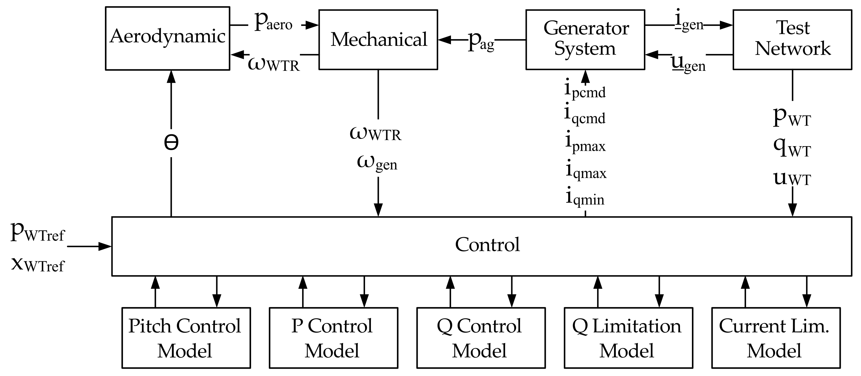
2. IEC 61400-27-1 Generic Type 3 WT Model

The generic Type 3 WT model can be divided into two sub-models: Type 3A and Type 3B. The main difference lies in the generator system, which includes a protection system in the case of the Type 3B WT. This protection system is modeled through a set of dynamic blocks that decreases the current signals to zero when a voltage dip occurs. In the present work, as the field measurements were recorded on an actual DFIG WT in operation, the generic Type 3B is the model studied.
The generic Type 3B WT model developed by Standard IEC 61400-27-1 (hereinafter referred to as Type 3) consists of several sub-models, as shown in Figure 1: aerodynamic control model [22], which provides the two-mass mechanical model with the aerodynamic power ( p aero ) coming from wind; pitch control model [23], which calculates the value of the pitch angle ( θ )-position angle of the WT blades—required to follow the rotor speed and power generation setpoint ( p WTref ); two-mass mechanical model [24], which models the actual gearbox representing both the low-speed and the high-speed sides and provides the wind turbine rotor and the generator rotational speed ( w WTR and w gen , respectively); active power control model [16], which provides the generator system with the active current command ( i pcmd ) and also calculates both the reference rotational speed and the active power order; reactive power control model, which controls the reactive power injection through the calculation of the reactive current command ( i qcmd ) based on the user-defined reactive power reference ( x WTref ); reactive power limitation model, which provides the reactive power control model with the reactive power injection’s maximum and minimum dynamic values allowed at the wind turbine terminals (WTT); current limitation model, which calculates the limit values of both the active and reactive currents ( i pmax , i qmax and i qmin ); and generator system, equipped with a crowbar model [25,26,27], which has as output signals the active and reactive currents injected into the grid through a current source ( i gen , and the generator air gap power ( p ag )). Measured values of voltage ( u gen and u WT ), as well as active and reactive power ( p WT and q WT ) at the test network are also required as input signals in some control models. The single-line diagram of the generic Type 3 WT model is available in [8].
As discussed in Section 1, International Standard IEC 61400-27-1 states that there should be no differences when studying the responses of generic WT models using different software tools. However, there may exist differences in the implementation and initialization processes, as well as in the algorithms used by the simulation tools. Moreover, although the time step used during the simulations may be set as fixed when conducting the comparison between models implemented in different software tools, some of them use variable-step solvers, adjusting the time step depending on the variability of the signals.
IEC 61400-27-1 also describes the limits of the accuracy of the generic WT models [8]. Since the model’s accuracy is analyzed comparing simulation responses with measured data, errors in both cases may appear. On the one hand, regarding simulation responses, errors occur, as during the development of the standard, some simplifications were implemented in order to obtain technically simplified dynamic WT models, which are, nevertheless, accurate enough to represent the existing wide range of actual WTs. On the other hand, limits to possible model accuracy may also arise from the measurements. When performing transient stability analyses, electromagnetic phenomena are not of interest, and are thus not emulated and represented by the generic WT models. For instance, if the high voltage side of the transformer is chosen to perform the measurements, electromagnetic phenomena caused by the behavior of the transformer may be reflected in the measured data. The accuracy of the model will thus be lower. Furthermore, some errors and limitations are also generated when performing the measurements at actual WPPs or test benches. Deviations resulting from tolerances or bandwidth limitations of the measurement equipment, as well as errors derived from the measurements’ conversion, lead to cumulative errors in some measured signals. When converting from instantaneous values to root mean square (RMS) values to perform the comparisons, some errors also occur.
In view of the above, it is clear that there will exist errors between measurements and simulated data. For this reason, they must be correctly assessed and calculated according to IEC 61400-27-1 guidelines. Deviations between the responses of the two simulated models (PowerFactory and MATLAB) will also be assessed during this work, with the aim of identifying the main factors that cause them. The following subsections describe, on the one hand, the calculation process of the validation errors established by IEC 61400-27-1, and, on the other, the general implementation process followed by both simulation software tools used, also showing some of the dynamic control models that are part of the generic Type 3 WT, highlighting the particularities and adaptations required in each case.

2.1. Validation of Generic Models Based on IEC 61400-27-1 Guidelines

The validation process of the generic models involves several steps. First, the definition of the dynamic simulation model must be performed. Second, field measurements are needed to measure the responses of actual WTs. Thus, in order to perform the field tests, a fault-ride through (FRT) mobile test unit was installed in a Spanish wind farm during a measurement campaign led by the manufacturer Siemens-Gamesa. The connection of the test unit was made between the switchgear and the high voltage side of the power transformer of the WT. Further information regarding the FRT mobile test unit can be found in [25,28], since similar units have been used to analyze the FRT capability of WTs. Once the voltage dips were applied to the WT, the rate of the measurement sample was set to 10 kHz, and the measurements composing each data set began 10 s before the voltage dip was applied and ended 15 s after this point in time. This period is enough to carry out the measurements, since the transient stability responses of the simulation are reflected during that period and can then be properly assessed. After that, measurements of the events conducted are replicated in the WT model, so that the simulation data and the field measurements can be compared. Finally, the validation errors are estimated. In this regard, the most significant disturbances in power systems that lead to integration issues are voltage dips [29]. In terms of RMS values, voltage dips involve severe voltage reductions ranging between 10% and 90% and a duration of up to one minute [19,30]. Residual voltage (minimum value of voltage) and dip duration are the two parameters that characterize these types of disturbances in the grid. However, the complexity of WTs means that not all kinds of voltage dips are suitable to be conducted on actual WTs, and, hence, IEC 61400-21 established a representative set of disturbances in order to validate a WT model [17].
As explained in Section 1, only a few scientific studies have performed validation tasks using field measurements, and even fewer when it comes to the implementation, simulation and validation of the most widely used type of WT, Type 3 (i.e., DFIG), in specialized software tools. Moreover, this study presents a triple comparison, which involves field measurements and simulation results from the same generic WT model implemented in two different tools. It also provides information, for the first time, about the slight deviations that may exist between those simulation results, despite IEC 61400-27-1 indicating they should not exist. This comparison thus helps to further determine the limitations of the IEC-developed WTs, in addition to achieving a more widespread use of these models.
In order to be able to obtain a response and a well-founded and justified conclusion, and based on the objectives previously mentioned, the criteria used to validate the generic WT models with field measurements, defined by IEC 61400-27-1, were also applied when comparing the simulated models with each other. Three time windows are defined during the simulation: (i) pre-fault window, which starts 1000 ms before the fault initiation, (ii) fault window, which lasts from the onset to the clearance of the fault, (iii) post-fault window, which lasts 5000 ms after the voltage dip clearance. Furthermore, in order not to consider transient periods in the assessment of the accuracy of the models, several time sub-windows are also defined, formerly known as ’quasi-steady state’ sub-windows. Hence, the transient responses appearing at the start of both fault and post-fault windows are discarded in the calculation of the maximum errors, as will be seen later in this document. On the one hand, a transient period of 140 ms is not considered in the calculations of the maximum validation errors at the start of the fault window due to the limitations of the generic model in reproducing the DC-component of the generator flux [12]. On the other hand, since the model is unable to faithfully represent the transformer inrush current, thus affecting the active and reactive power responses, a period of 500 ms is not considered at the start of the post-fault window. In addition, it is worth considering that, because of the inability to model the aerodynamic oscillations or nonlinear aerodynamic effects by generic WT models, larger errors may occur during the entire post-fault window. Figure 2 shows both the time windows and the quasi-steady state sub-windows defined during the voltage dip according to [8].
The calculation of validation errors during the pre-fault window is not critical for the evaluation of the performance of the model. Therefore, error time series are only calculated during fault and post-fault windows for each of the comparisons ( x e r r o r in Equation (1)), i.e., between the data series of the following cases: (i) MATLAB Model–Field Data, (ii) PowerFactory Model–Field Data, (iii) MATLAB Model–PowerFactory Model. On the basis of this information, three validation errors (also referred to as validation performance indicators) are calculated in both fault and post-fault windows, the calculations of which are presented in Equations (2)–(4): Mean Error (ME), Mean Absolute Error (MAE) and Maximum Absolute Error (MXE) [12].
In Equations (1)–(4), numbers 1 and 2 indicate the data series to be compared in each case, while n indicates the indices of the vectors and N the total number of samples used:
x e r r o r ( n ) = x 1 ( n ) x 2 ( n ) ,
x M E = n = 1 N x e r r o r ( n ) N ,
x M A E = n = 1 N | x e r r o r ( n ) | N ,
x M X E = m a x ( | x e r r o r ( n ) | ) .
ME is defined as the mean value of the error over the corresponding time window, and is related to the steady-state performance of the dynamic model; MAE is the mean value of the absolute error, calculated over the entire time window in the case of the post-fault period, and over the corresponding quasi-steady state sub-window in the case of the fault period; and, finally, MXE is the maximum value of the absolute error, mainly related to the transient performance of the simulated model. In this last case, the quasi-steady state sub-windows are considered in the calculation. The electromagnetic transient periods measured are thus not considered in the evaluation of the accuracy of the model, since fundamental-frequency generic models are not designed to represent them. As a summary, Table 1 shows the time periods considered for the calculation of each type of error in both the fault and post-fault periods, according to Figure 2.
Having explained the validation criteria to be applied, the following sections are devoted to describing, in general terms, the generic Type 3 WT modeling process in the two software tools used.

3. Modeling Process of Generic Type 3 WT

The structure of the generic Type 3 WT and the validation process that must be followed to test its electrical performance have been extensively described in previous sections. Moreover, limitations to the model’s accuracy included in IEC 61400-27-1 have also been listed. However, with the objective of achieving well-reasoned explanations of the causes of the differences in the model’s behavior when it is simulated in the two software tools, the ways in which the dynamic WT model is implemented are described in detail below.

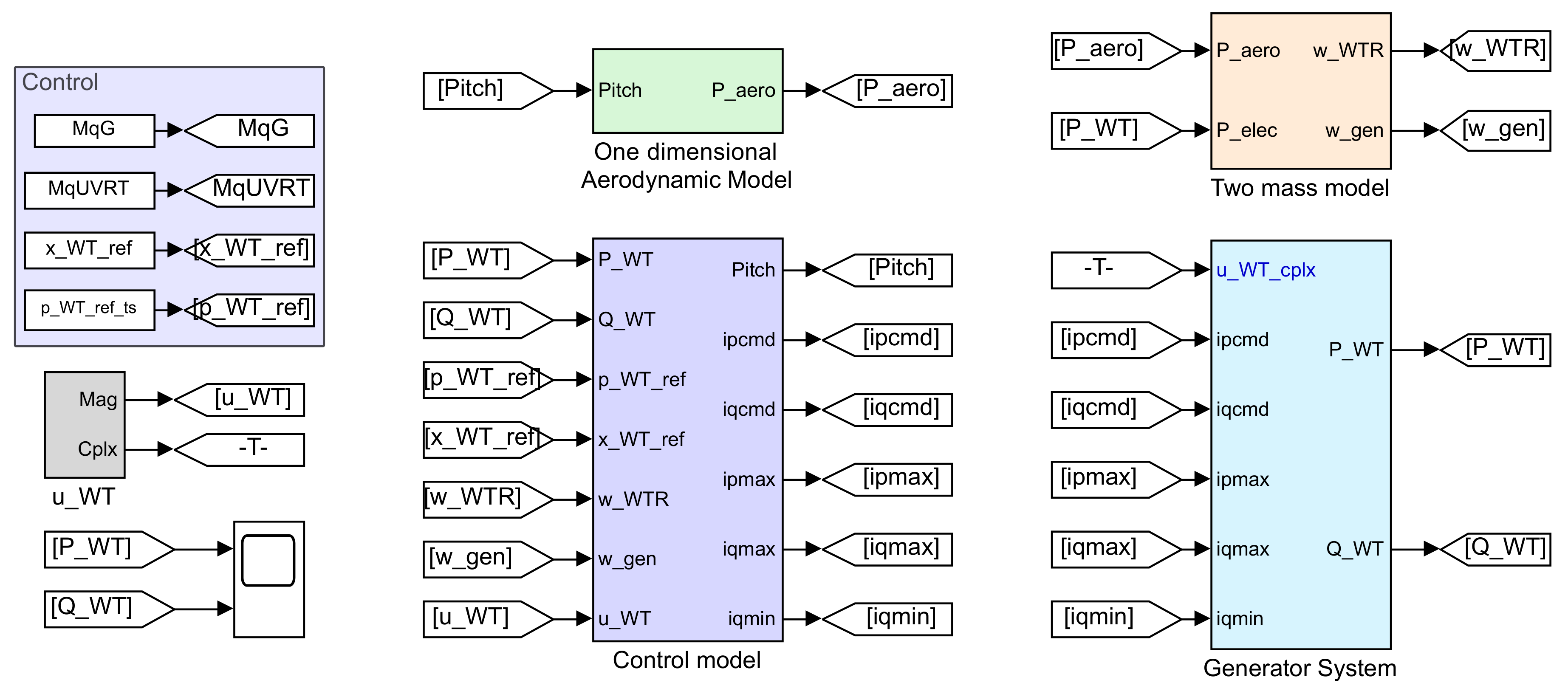
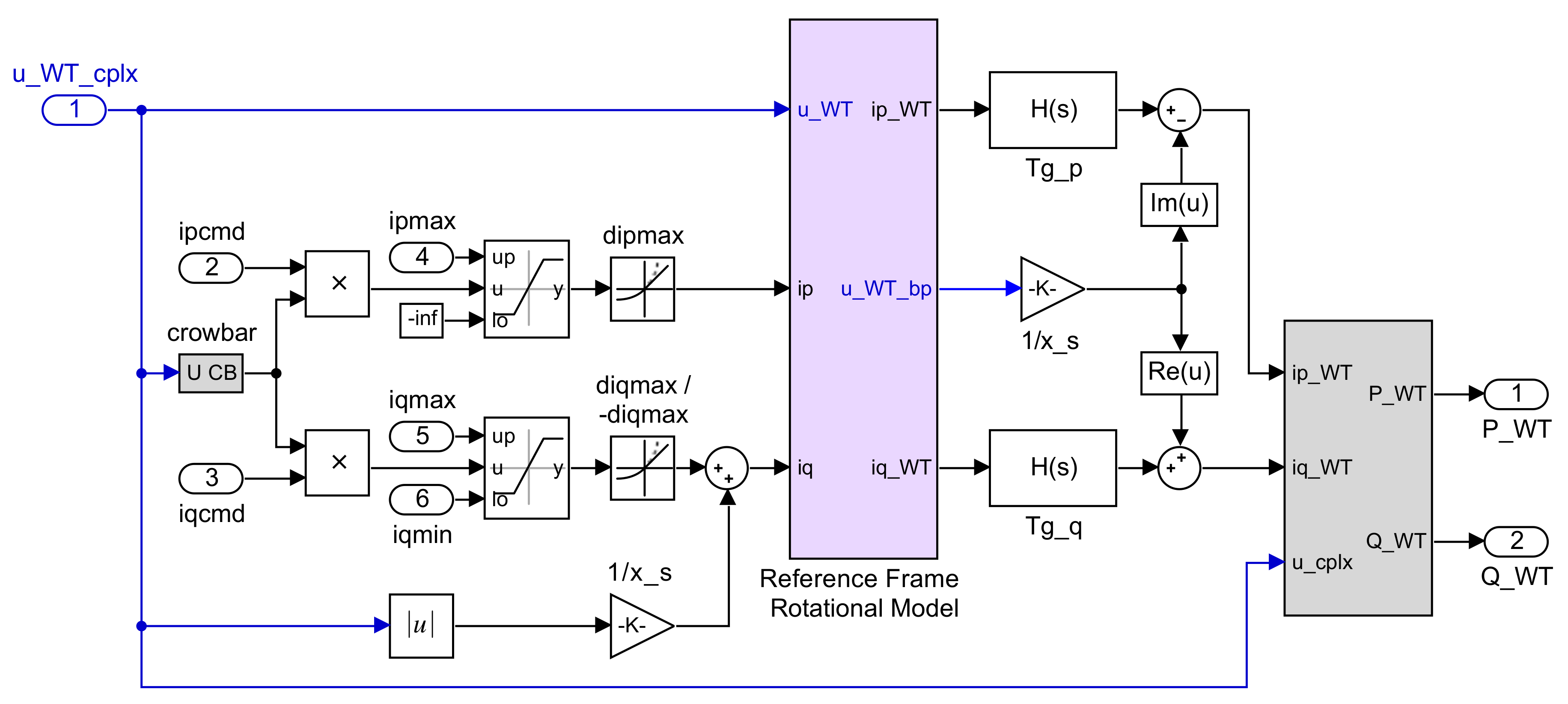
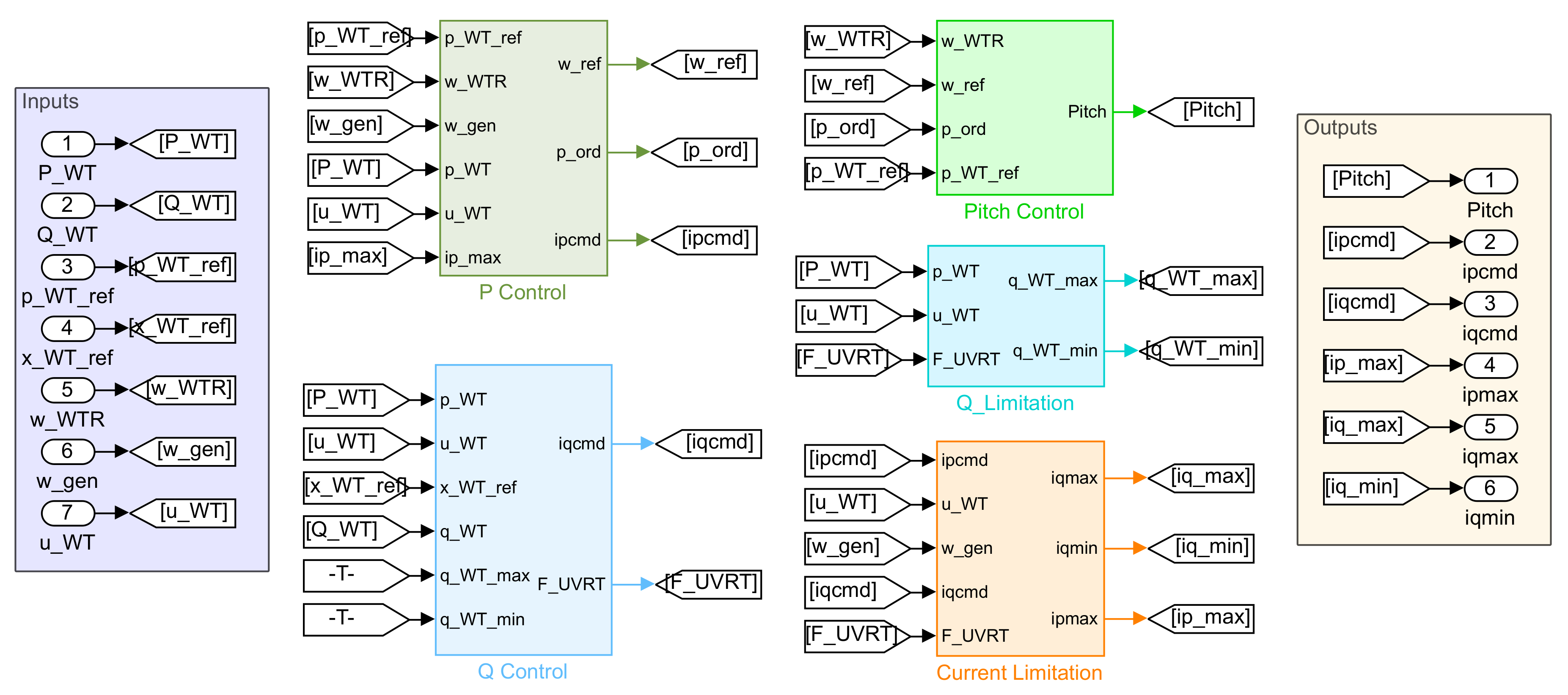
3.1. Implementation in MATLAB/Simulink

MATLAB/Simulink is currently one of the most widely used software tools in engineering. Its flexibility, supported by its large community, allows a wide range of studies to be conducted. Furthermore, with the addition of Simulink, its add-on, which works with block language, the possibilities are unlimited. For this work, the generic Type 3 WT model was first modeled and parametrized in Simulink, as the facilities included permit faster development. Furthermore, the validation work was conducted in MATLAB, the programming language of which permits easy implementation of the IEC 61400-27-1 validation methodology described in Section 2.1.
Regarding the IEC 61400-27-1 generic Type 3 modeling, its general structure is shown in Figure 3. Additionally, the systems included within the ‘Control model’ are shown in Figure 4. The control of the generic Type 3 model has previously been explained in the literature. In [17], the behavior and parametrization of the systems related to the active power response is explained. Furthermore, in [31], the behavior of the reactive power control, the current limitation system and the generator system are depicted and compared with a simpler model [32].
The electrical generator system is one of the most complex in this Type 3 WT model. It is based on the physical dynamics of a DFIG, and the theory behind its development is described in [10,15]. For the present work, as explained in Section 2, the authors modeled a generic Type 3B electrical generator system, which includes the crowbar protection system. Its modular structure is shown in Figure 5. The ‘reference frame rotational model’ coordinates the active and reactive command currents with the grid reference frame. Furthermore, this system includes the dynamics of the generator sub-transient reactance x _ s . Additionally, the crowbar system is modeled as a system that multiplies by 0 the command currents over a short time when the fault occurs and ends, depending on the derivative of voltage. Finally, as shown in Figure 3, the Simulink model is not connected to a grid. The active and the reactive power are calculated based on Equation (5):
S ¯ WT = P _ WT + j Q _ WT = U ¯ WT I ¯ WT * = u WT φ u _ WT · ( i p _ WT + j · i q _ WT )
Additionally, it should be mentioned that the fine adjustment of the model parameters was conducted using the Simulink Design Optimization tool. An example illustrating the use of this tool is shown in Figure 6. For this work, the reference signal was either the active or the reactive power response. Then, the parameters that we wish to adjust are selected, as well as their ranges and scale. Finally, the program iterates until reaching the objective selected. The iteration method and the error followed (absolute or relative) can be selected. Finally, the software provides the finely adjusted parameters. As a side note, although this process might seem automatic, the approximately 100 parameters which define the generic Type 3 model means the user can have a deep understanding of the behavior of the model, as well as the parameters which should be adjusted and their logical ranges in which to conduct the tuning.

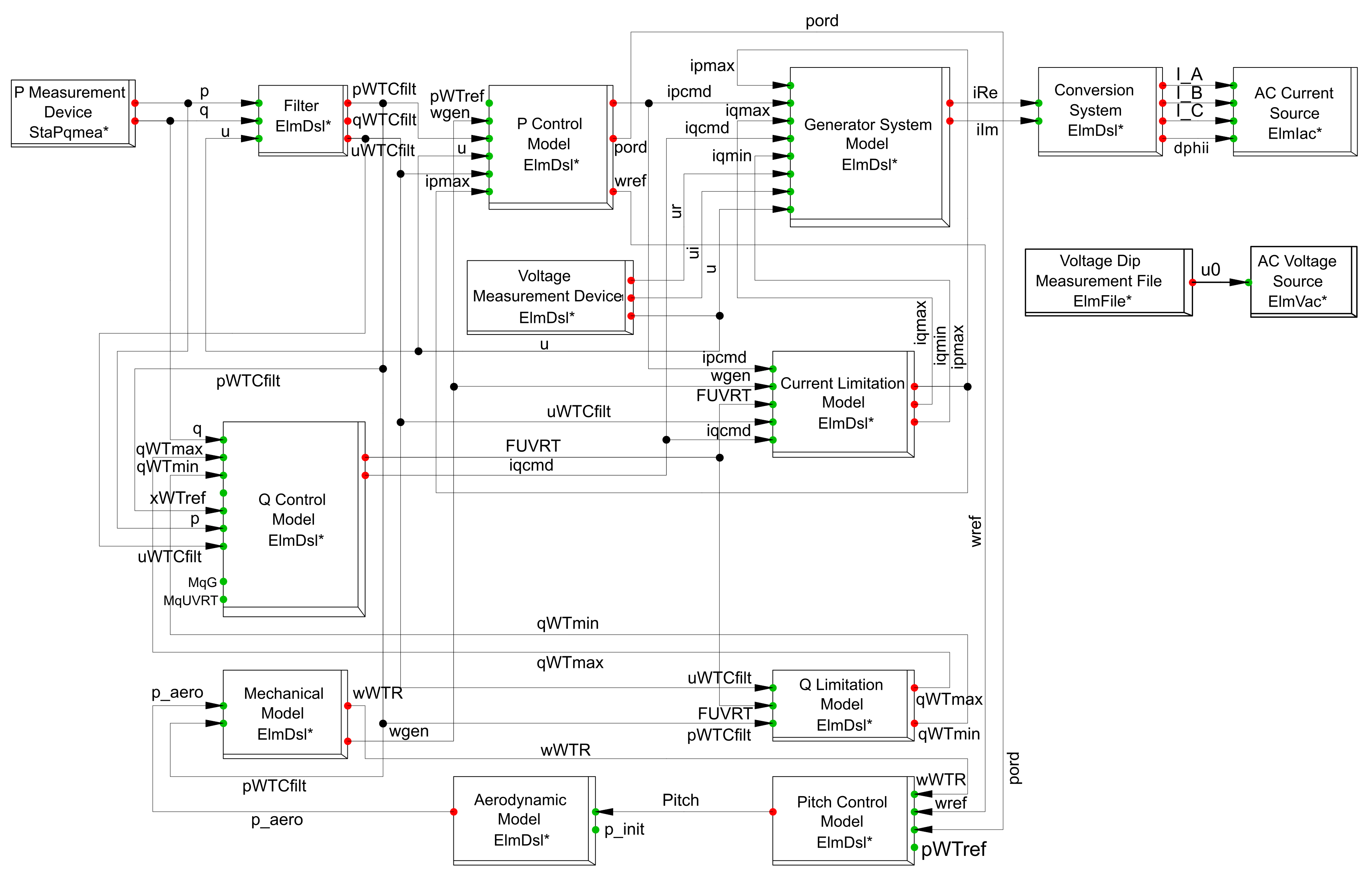
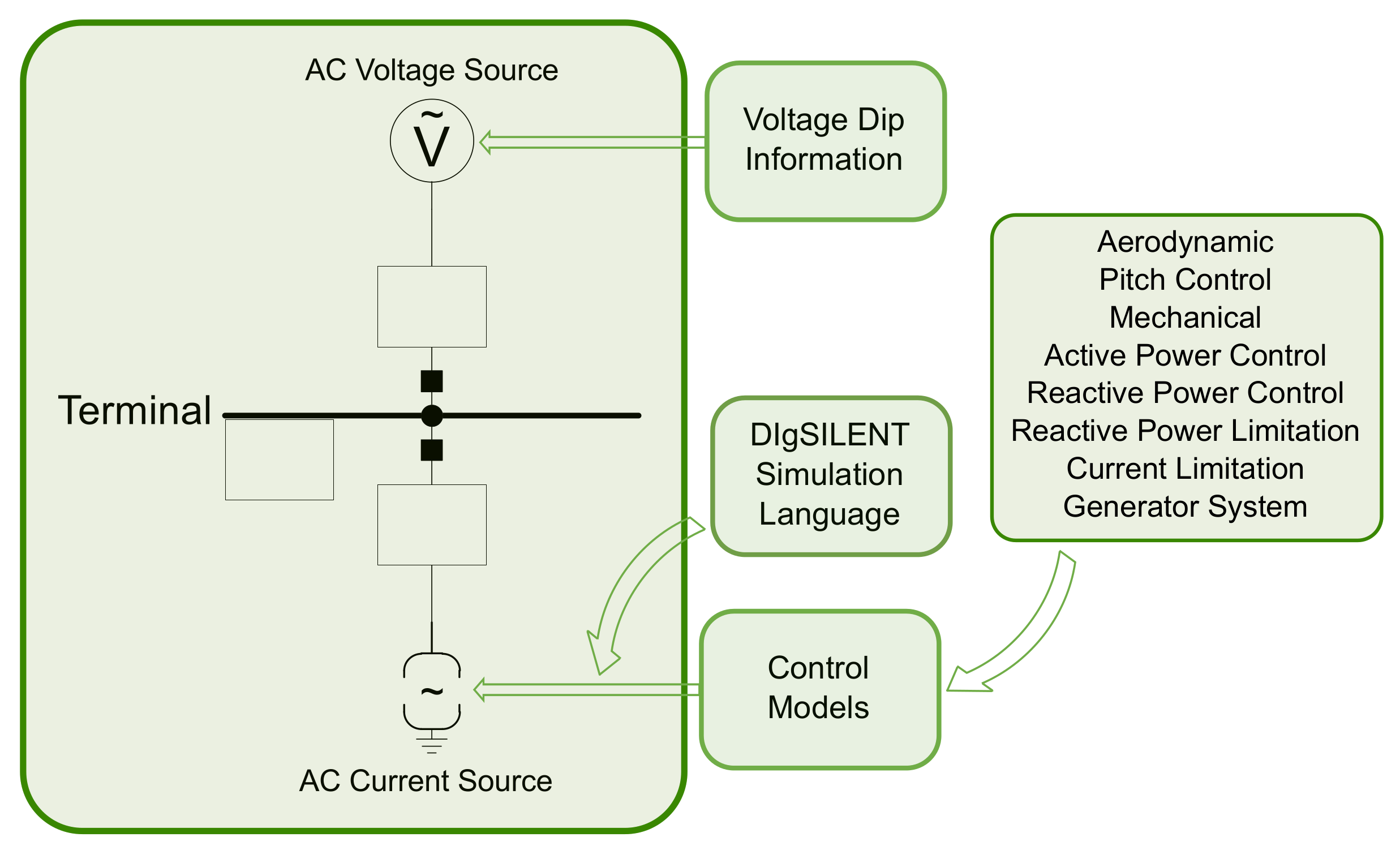
3.2. Implementation in DIgSILENT-PowerFactory

The previous sections highlighted the importance of using specialized electrical engineering software tools, as they permit a wide range of studies to be carried out. In addition, these types of tools allow highly complex studies to be performed, enabling also the consideration of the vast amount of information and the large number of parameters which characterize actual power systems [33]. It is therefore of prime importance to have in-depth knowledge of the dynamic model’s implementation process, and an overview of particularities of the software and also of the calculation method or the network representation, as these will help to further understand the causes of the deviations between simulation results provided by the two software tools. The way in which voltage dips are conducted at the WT model implemented in DIgSILENT-PowerFactory (PF) is also an important element.

3.2.1. DIgSILENT Simulation Language

DIgSILENT Simulation Language (DSL) is the PF function used to model dynamic systems [34]. When working with DSL, predefined electrical devices available in the software and user-defined dynamic blocks may be incorporated into the power system, i.e., complete dynamic models are implemented in PF by relating a certain electrical component with its corresponding control models, influencing its electrical behavior. In fact, the WT is modelled as an AC current source that injects active and reactive current into the grid. Active and reactive power are thus measured through a predefined power measurement device connected at the WTTs, while a conversion system has been specifically designed to adapt the output current signals from the generator system model to the input signals’ format required by the AC current source.
Based on [8] and the DSL working structure [35], Figure 7 shows the complete power system implemented in PF, which relates all the generic Type 3 WT dynamic models described at the start of Section 2, including the AC current source representing the WT and measurement and auxiliary devices.

3.2.2. Time Domain Simulations in DIgSILENT-PowerFactory

The initialization of the power system is of great importance, since correctly executing the initialization process avoids fictitious electrical transients and allows the system to rapidly reach the steady-state condition [36]. Otherwise, numerical instability may appear [33]. First, a load flow calculation to initialize the predefined electrical components must be executed. Second, the equations of the initial conditions must be set manually in every user-defined DSL dynamic model (based on the information provided by the load flow calculation) [37]. Finally, the ’calculation of initial conditions’ command must also be executed.
’AC Load Flow, balanced, positive sequence’ is the calculation method followed. It performs the calculation for an equivalent single-phase, i.e., for a network representation of positive sequence. This method is valid in the case of balanced symmetrical networks, which justifies the subsequent choice of the simulation method. Therefore, for the calculation of initial conditions, the balanced RMS simulation method, which considers a steady-state, symmetrical representation of the electrical grid, is selected. Dynamics in electromechanical and control devices are thus taken into account, and only fundamental components of voltages and currents are considered [34]. Under these conditions, only symmetrical faults are allowed. Indeed, generic WT models defined by IEC 61400-27-1 are designed to conduct studies of three-phase symmetrical faults.

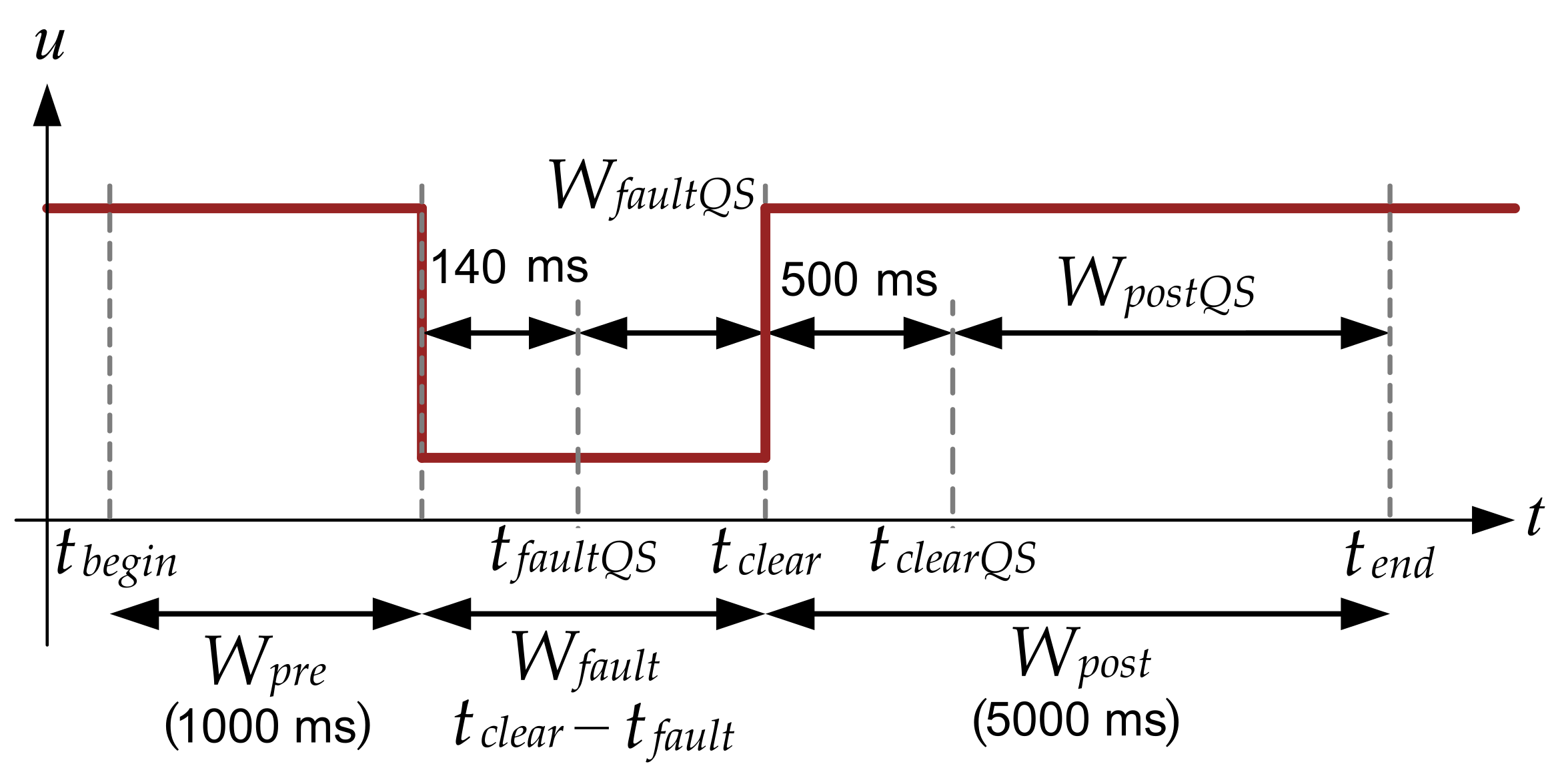
3.2.3. Conduction of Voltage Dips at the WTTs

Once the complete power system is initialized, it may generally be studied under two different operating conditions: normal and fault operating conditions. However, as stated in Section 1, electrical disturbances such as voltage dips are the most critical situations to be assessed in order to allow network operators to properly plan system operation. Hence, since this study aims to calculate validation errors between field data and the results of generic Type 3 WT model simulation by reproducing two voltage dips measured on an actual WT in operation, the play-back validation approach was used [38]. Instead of conducting a voltage dip by defining a short-circuit at one of the WTTs [35], an external AC voltage source was connected to the WT model. This voltage source is controllable through a voltage dip measurement file and positive sequence voltage values are used as the input signal. In this way, the power system is forced to behave under the desired conditions. The play-back method thus constitutes the most suitable approach in such cases, as it enables the accurate reproduction of voltage dips that correspond to field measurements (see dynamic sub-models ’Voltage Dip Measurement File’ and ’AC Voltage Source’ in Figure 7).

3.2.4. Test Network

The AC current source to which the control models are connected and the controllable AC voltage source reading the voltage dip measurement file are part of the same test network. Considering that this work is focused on comparison studies and calculation of validation errors, as well as on the analyses of the Type 3 WT’s electrical responses in isolation, strictly equal voltage profiles must be considered in the cases analyzed (in MATLAB and PowerFactory). Therefore, it is not important to go into depth in the test network as it does not represent an actual power system, nor does it affect the performance of the generic WT model, since it has only been defined to be able to reproduce the voltage dip measured at the actual WT and assess, in such a way, the accuracy of the simulation responses.
However, both the current and voltage sources need to be physically connected because they are predefined electrical devices in PowerFactory, with a test network such as the one presented in Figure 8 being the modelled auxiliary power system. It consists only of the sources of the AC current and voltage and a terminal interconnecting them. Figure 8 is also a schematic illustration of how dynamic control models are related to the AC current source through the DSL.

4. Results

This section presents a comparison of the responses of the generic Type 3 WT model implemented in both software tools during two different voltage dips, and also the calculation of the validation errors according to Section 2.1. Moreover, it performs a comprehensive analysis of the reasons for such errors. The values of the main parameters that are part of the generic Type 3 WT model are shown in Table 2.

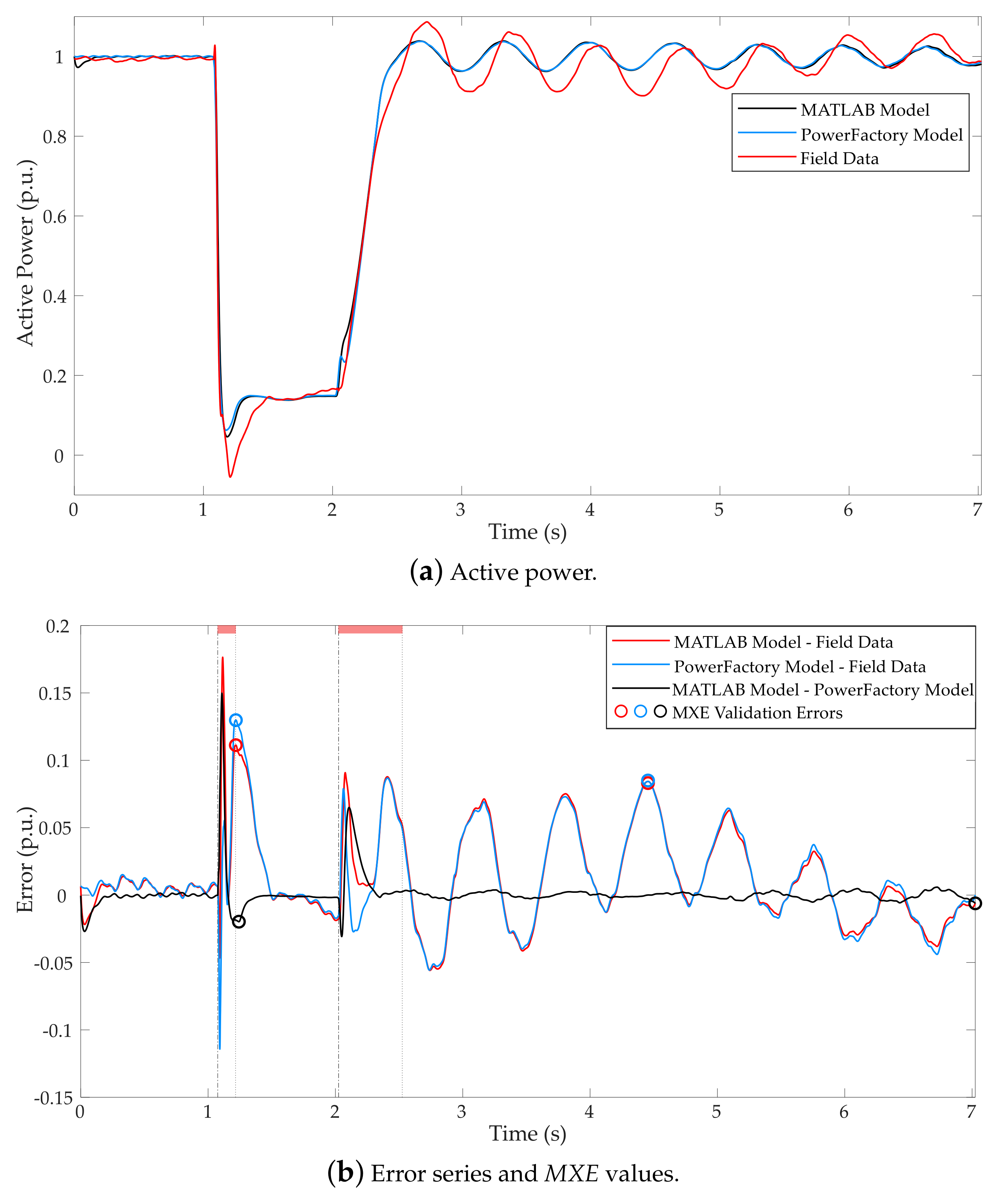
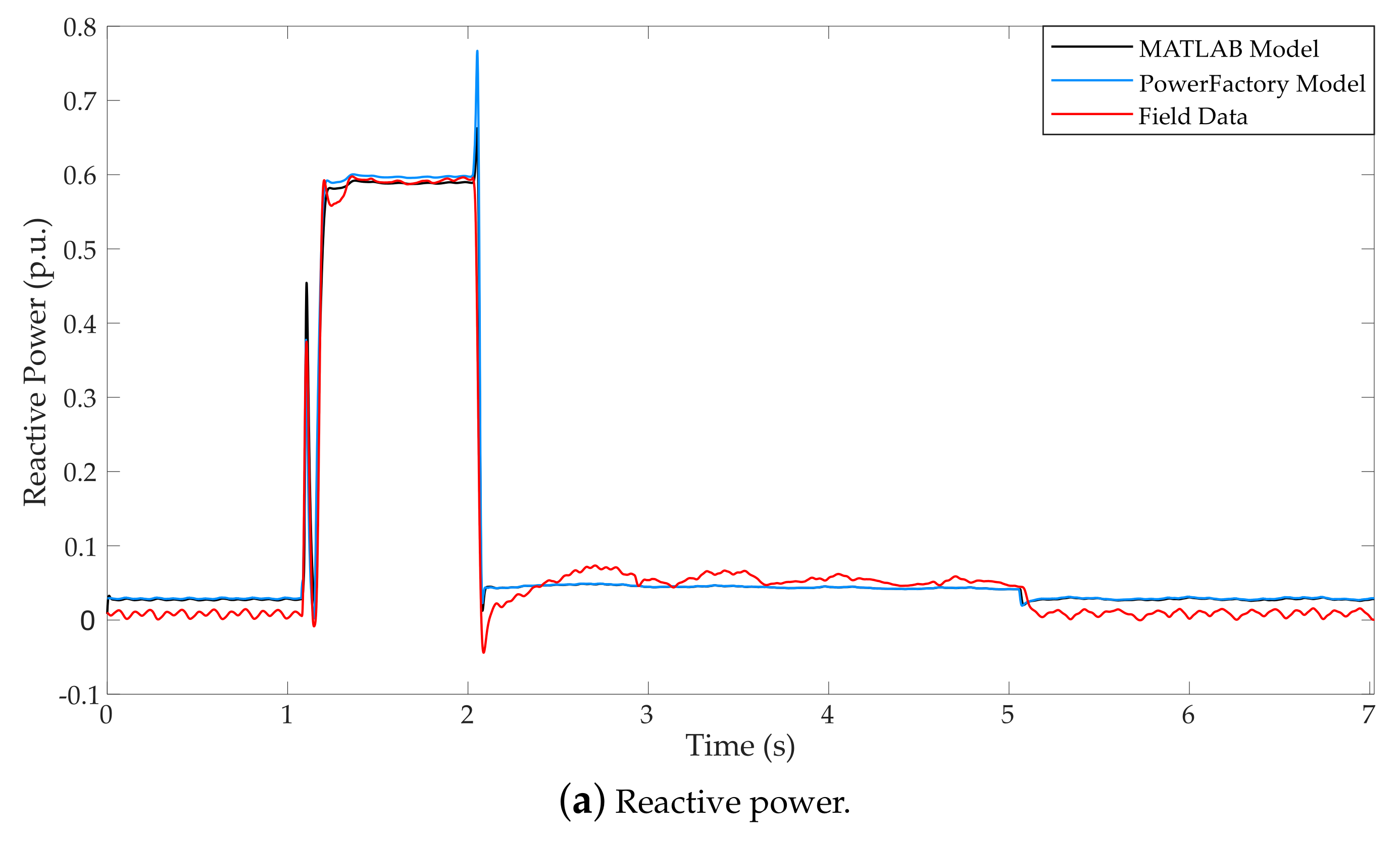
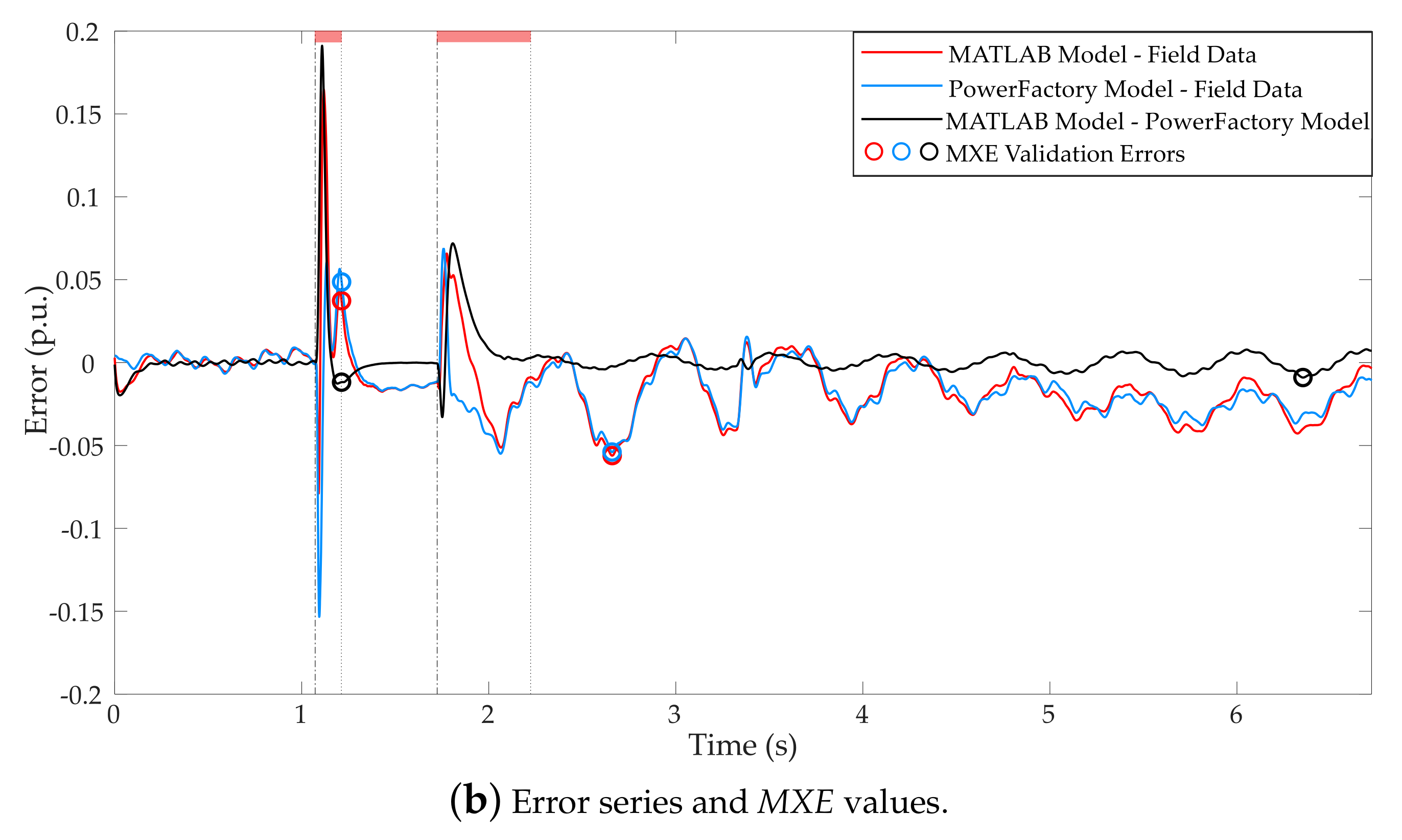
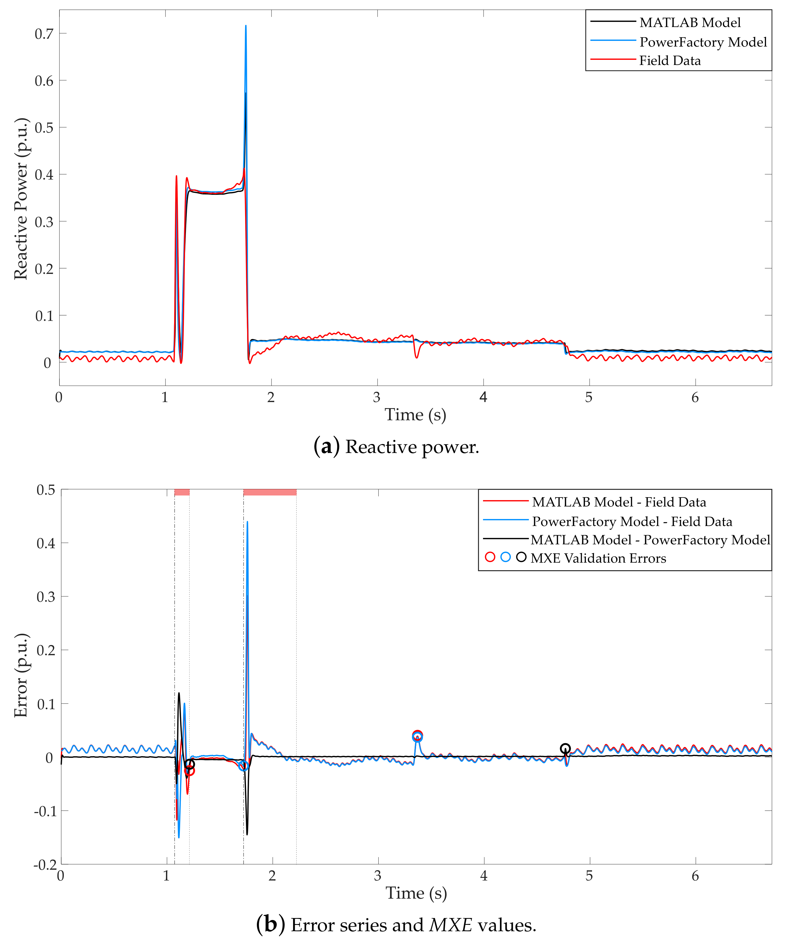
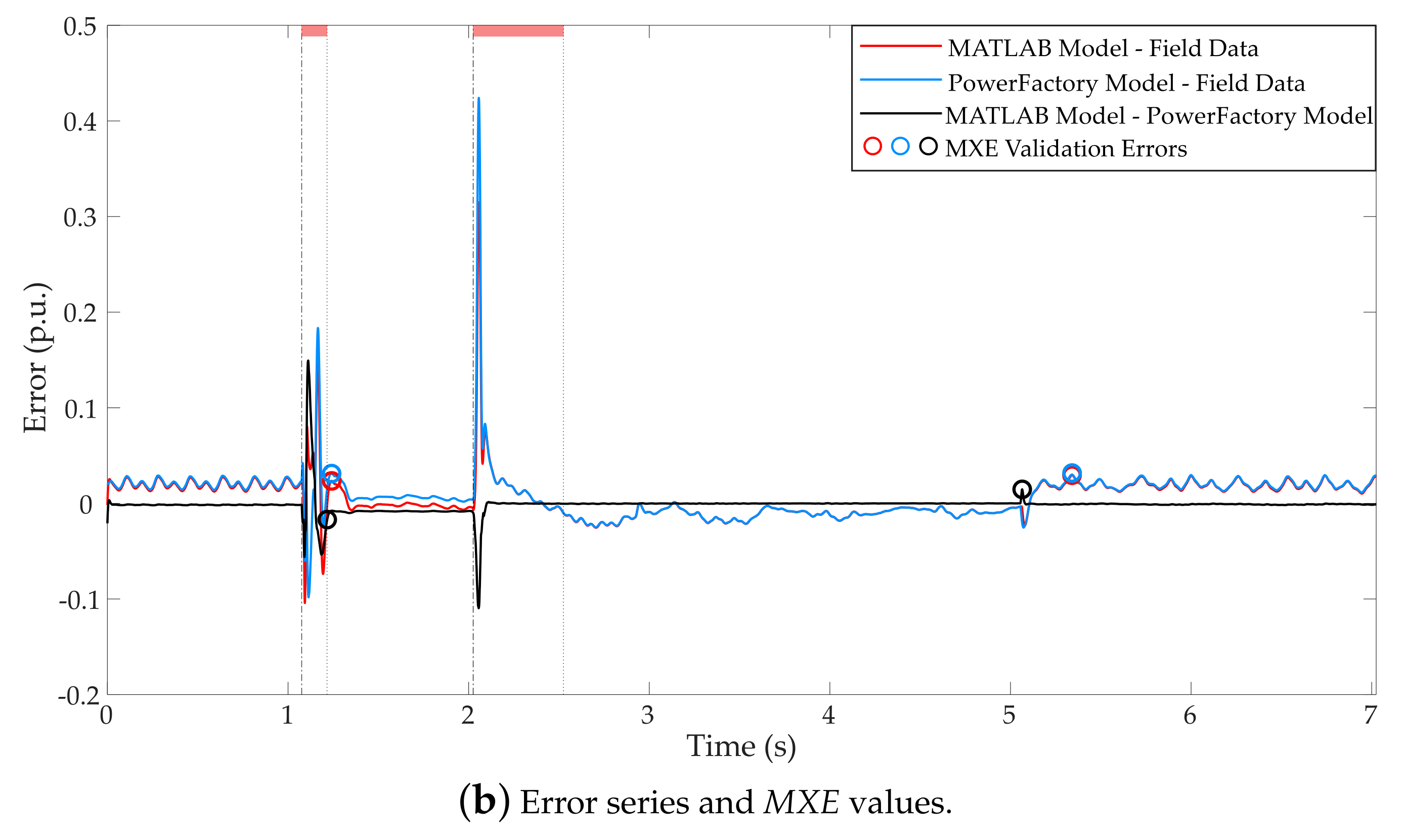
4.1. Validation of the Generic Type 3 WT Model

The WT dynamic model (implemented in MATLAB/Simulink and DIgSILENT-PowerFactory) was submitted to two different voltage dips, the residual voltage (u), and dip duration (t), of which are u = 0.50 pu and t = 920 ms for the Test Case 1, and u = 0.25 pu and t = 625 ms for the Test Case 2. In order to do so, the field data series were converted to positive sequence values, since the generic WT models must be studied for fundamental frequency-positive sequence response analyses. Thus, the positive sequence values of the voltage dips were reproduced in the generic WT models.
Figure 9 and Figure 10 show the active and reactive power responses and their validation errors in Test Case 1, while Figure 11 and Figure 12 show those corresponding to Test Case 2. The value of the more than a hundred parameters which are part of the generic Type 3 WT model do not vary from one software to the other. This explains the excellent correlation between the two simulation data series (in blue and black), in both the active power (Figure 9a and Figure 11a) and the reactive power (Figure 10a and Figure 12a), for both Test Cases. In these figures, a red line represents the measured data from the field tests. As might be expected, the differences between measured and simulation data are higher than the differences between both simulation responses, despite the generic Type 3 WT model having been adjusted to the field data series to the maximum extent.
In the graphics of the error data series, Figure 9b, Figure 10b, Figure 11b and Figure 12b, vertical lines and red bars at the top indicate the transient periods of 140 ms and 500 ms that must not be considered in the calculations of errors at the start of fault and post-fault periods, respectively, as explained in Section 2.1. As can be observed in these figures, error lines between simulation models and measured data for all cases (in red and blue) show sharp peaks. In addition, Figure 9 shows how an aerodynamic imbalance may affect the error between the field data and the simulation responses. The real response shows an undershoot during the post-fault period due to a wind speed fluctuation, which can be emulated by neither of the generic WT models. Nevertheless, as will later be explained drawing on Table 3 and Table 4, the maximum errors obtained do not exceed 13% in either case (the MXE values are marked in the figures as small circles). Finally, the black lines represent the error obtained between both simulation models, which is at around 0% in all cases.
In general, the graphic representation of the errors obtained is a good way to provide a general but comprehensive overview of the results. Thus, a quick glance reveals the performance of the simulation models, since the higher the deviation from 0%, the lower is the accuracy of the simulation models compared with each other and with the field measurements.
Furthermore, the numerical results of the validation errors are presented in Table 3 for Test Case 1 and Table 4 for Test Case 2. Different trends may be observed. First, as expected, lower errors are obtained for the ’MATLAB-PowerFactory’ comparison (third column of Table 3 and Table 4), since the behavior of both simulation models is very similar. In these cases, the ME and the MAE do not exceed 1% either in the active power or in the reactive power of the two test cases analyzed, in both fault and post-fault periods. Regarding the MXE, it does not exceed 2% in either case for the ’MATLAB-PowerFactory’ comparison. It can therefore be stated that, despite the slight deviations which will be analyzed in Section 4.2, there is very little difference between the MATLAB and the PowerFactory simulation responses.
In light of the above, the values of the errors between the ’MATLAB-Field’ and ’PowerFactory-Field’ data series are very similar, as can be observed in Table 3 and Table 4. Moreover, in general, the ME, the MAE and the MXE are lower in the reactive power responses than in the active power responses for both test cases. This means that the reactive power simulation response of the generic Type 3 WT model is better adjusted to the field measurements. Despite this, there also exists a good correlation between the simulation and the field measurements in active power for both test cases.
Hence, as the generic WT models developed by IEC 61400-27-1 are not intended to be studied during the transient periods appearing at the start and the clearance of the faults, higher error values may be obtained. Indeed, most of the MXE errors obtained are near the transient periods of the responses (see the small circles in Figure 9b, Figure 10b, Figure 11b and Figure 12b and the red bars at the top, respectively), where the accuracy of the model with regard to the field measurements is usually lower. This is because transient periods of the actual WTs are not adequately represented by the generic models.
The efficient performance of the simulation models is also supported by the good correlation in the amplitude and the phase shift of the active power responses after the voltage dip clearance (Figure 9a and Figure 11a). This is mainly due to the good fit to the parameters of the two-mass mechanical model. Moreover, the reactive power responses provided by the generic WT models are highly accurate (Figure 10a and Figure 12a), since they present a very similar behavior to that of the field measurements (including the reactive power injection period during the voltage dips to stabilize the voltage).
Therefore, in view of the explanations above and the low values of the validation errors obtained, it can be concluded that the simulation responses of the generic Type 3 WT model yield satisfactory results, since, on the one hand, both emulated responses are very similar (with errors around 0%) and, on the other hand, both models are adjusted adequately to the field measurements.

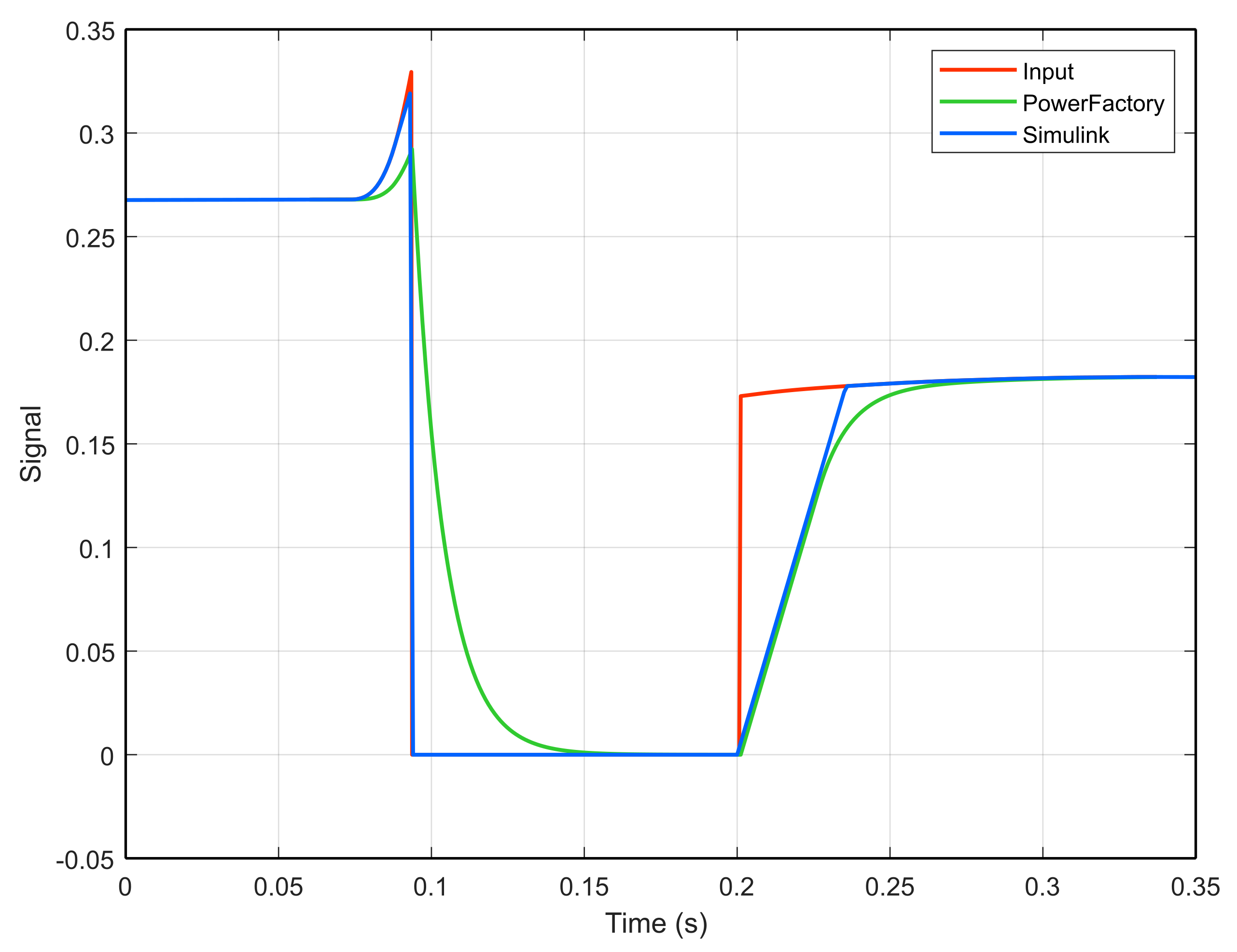
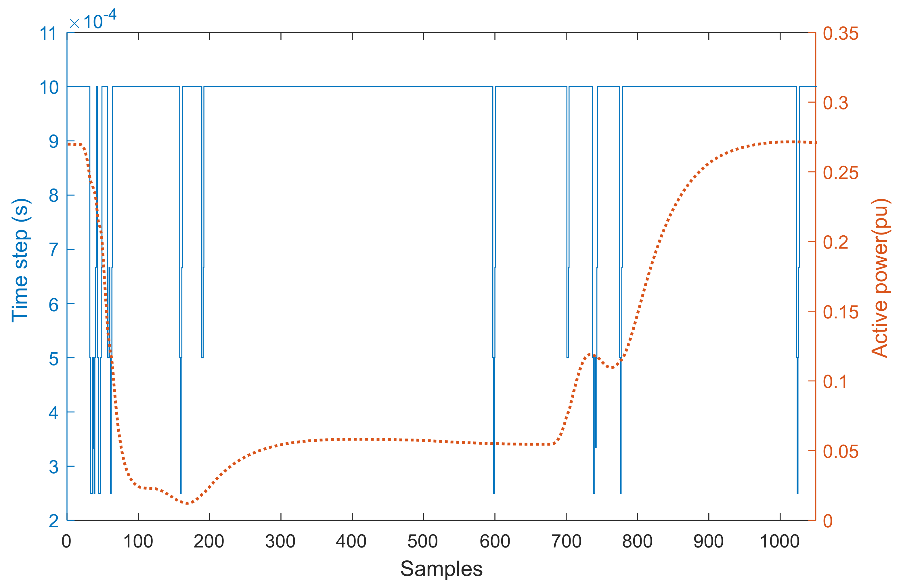
4.2. Analysis of the Limitations of the Software Tools: Causes of the Differences in the Simulated Response

Section 4.1 analyzed the values of the validation errors calculated according to the validation guidelines issued by IEC 61400-27-1 in the three cases considered: (i) MATLAB Model—Field Data, (ii) PowerFactory Model-Field Data, (iii) MATLAB Model—PowerFactory Model. This section aims to explain the main differences in the software tools that may cause the errors found between both simulation responses of the generic WT model. However, it is worth noting that the validation errors are smaller than 2% for all cases. The explanations included in this Section intend to clarify the small differences between both simulation responses (from the two software tools used) at the time of conducting dynamic simulations, but always considering that the results are equally valid for both of them.
Figure 13 shows one of the constraints when comparing both simulation tools. Specifically, the response of a signal passing through a built-in rate limiter in PowerFactory and Simulink is analyzed. The rising rate was set to 5 and the falling rate was set to −999. It can be observed that the PowerFactory response is not the expected behavior, while the Simulink response is correct. Basically, PowerFactory applies a first-order filter to the input signal of the block, the time constant of which can also be adjusted. Thus, setting a lower time constant should dampen the effect of this filter. Nevertheless, this filter has an effect on the signal and, hence, the responses from PowerFactory and Simulink when using these limiters (which are several in IEC 61400-27-1 models) are not the same. More precisely, the generic Type 3 WT model includes a total of five rate limiters, two in the generator system model and three in the active power control model, so that the combined effect of these blocks on the output signals also explains the differences between the responses of both software tools. These filters are not implemented in Simulink since IEC 61400-27-1 does not include them in the models.
Additionally, despite the PowerFactory solver being set to ‘fixed step’ with a time step of 1 ms, the time step varies during the simulations. Regarding Simulink, the solver was set to ode4 (Runge–Kutta) with a fixed time step of 1 ms. This type of solver is widely used due to its balance between accuracy and simulation time. This is shown in Figure 14, which represents the time step at each sample, as well as the active power response for that simulation. When the active power response varies greatly, the time step decreases to improve the accuracy. In fact, this is the appropriate behavior for a variable step solver. However, for comparison purposes, a real fixed-step simulation time would be desirable. Therefore, this variable time step used by DIgSILENT-PowerFactory for the simulation of the WT model was identified as another one of the main causes of the slight differences between the simulation responses of the two software tools.
Therefore, differences in the rate limiter responses in both software tools, and the variable time step used by DIgSILENT-PowerFactory during the simulation, are identified as the key factors explaining the errors between the responses of the generic Type 3 WT dynamic model.

5. Conclusions

Wind power will be the third largest renewable energy source around the world in 2023, and will provide approximately 30% of the total power demand during that year. However, this scenario gives rise to the problem of integrating the installed wind power capacity into the grid. Since the nature of wind is unpredictable, WPP installations are regarded as non-dispatchable, and hence TSOs and DSOs in different countries must carry out proper planning of network operation, and also forecast the participation of conventional power plants to compensate fluctuations in wind power generation. Moreover, voltage and frequency regulation problems may emerge in these situations.
In light of the above, transient stability analyses of WT and WPP dynamic models are required to forecast the electrical behavior of actual WTs before being connected to the grid. For this purpose, the International Electrotechnical Commission, through IEC 61400-27-1, defined four WT simulation models intended to represent actual WTs of different manufacturers. These generic WTs consist of a small number of dynamic sub-models and parameters, and may be implemented and simulated in any software tool. Moreover, the Standard states that the responses obtained must be the same and independent of the software used. The present work demonstrates that, nevertheless, there may exist deviations between the two sets of results.
In order to analyze these differences, the generic Type 3 WT model, i.e., the DFIG WT, was implemented and simulated in MATLAB/Simulink and DIgSILENT-PowerFactory. Although MATLAB is widely used in the scientific literature, more specialized software tools, such as PowerFactory, are often used by TSOs and DSOs in different countries. Thus, the present work contributes to achieving a more widespread use of the recently developed generic WT models, also benefiting all stakeholders in the wind power industry.
The models were subjected to two different voltage dips, and their active and reactive power responses were compared with field measurements from an actual WT in operation. Validation errors following IEC 61400-27-1 guidelines were also estimated. In this way, it has been demonstrated that both simulation software tools are equally valid for the development of generic WT models. Beyond the specific applications of each tool, numerical differences between them are smaller than 2% for all the validation errors. Thus, it can be concluded that generic WT models can be implemented in the simulation software tool that fits better to the needs of the user.
With regard to the validation study, in general, the validation errors obtained between the field data series and the active and reactive power simulation responses of the models implemented in both software tools are low. The slight differences are due, firstly, to the limits of the model’s accuracy, since, during the development of the Standard, some simplifications were introduced to design technically easy WT models (for instance, transient periods are not accurately represented by the generic WT models). Secondly, the errors may also be due to the limitations when the measurements were performed, such as the ones introduced by the tolerances of the measurement equipment, and also due to the conversion from instantaneous values to RMS values.
In addition, the errors between the two sets of simulated responses are near zero in the two Test Cases considered. Nevertheless, after carefully analyzing the differences in the implementation processes of both software tools and the behavior of each dynamic block, the errors between the active and reactive power responses may be attributed to two causes. The first cause could be the differences in the rate limiters used by the simulation tools. In these cases, PowerFactory applies a first-order filter to the input signal, the time constant of which affects its behavior and may dampen the effect of the filter. This affects the overall behavior of the WT, since IEC models use several of these rate limiters. The second cause concerns the time steps used. PowerFactory uses a variable step solver despite the time step being set as fixed. This may distort the dynamic responses of the WT model over time, since a fixed step solver is desirable for comparison purposes.
In summary, the outcomes of this work include the assessment of the advantages and disadvantages of the two power system simulation tools through the analysis of their implementation processes. Furthermore, the dynamic simulation of the generic Type 3 WT model is intended to provide a better understanding of IEC 61400-27-1, assessing its limitations and the accuracy of its originally-developed dynamic WT models, thus extending their field of application.

Author Contributions

Conceptualization, R.V.-R., A.L.-B. and E.G.-L.; Investigation, R.V.-R. and A.L.-B.; Methodology, R.V.-R., A.L.-B. and A.H.-E.; Project administration, E.G.-L.; Resources, F.J.-B.; Supervision, A.H.-E., F.J.-B. and E.G.-L.; Writing—Original draft, R.V.-R.; Writing—Review and editing, A.H.-E.

Funding

This research was funded by the Spanish Ministry of Economy and Competitiveness and European Union FEDER, grant number ENE2016-78214-C2-1-R, as well as the Agreement signed between the UCLM and the Council of Albacete to foster Research in the Campus of Albacete.

Acknowledgments

The authors would also like to express their gratitude to the wind turbine manufacturer Siemens Gamesa Renewable Energy for the technical support received. Furthermore, the authors would like to thank the TC 88/WG 27 Committee “Wind turbines—Electrical simulation models for wind power generation”, to his Convenor, Poul Sørensen, and to the 16 participating countries.

Conflicts of Interest

The authors declare no conflict of interest.

Abbreviations

The following abbreviations are used in this manuscript:
ACAlternating Current
DCDirect Current
DFIGDoubly-Fed Induction Generator
DSLDIgSILENT Simulation Language
DSODistribution System Operator
GWECGlobal Wind Energy Council
IEAInternational Energy Agency
IECInternational Electrotecnical Commission
MAEMean Absolute Error
MEMean Error
MXEMaximum Absolute Error
PFDIgSILENT-PowerFactory
PVPhotovoltaics
RMSRoot Mean Square
TSOTransmission System Operator
WPPWind Power Plant
WTWind Turbine
WTTWind Turbine Terminals

References

  1. IEA. Renewables 2018. Analysis and Forecasts for 2023; Technical Report; International Energy Agency: Paris, France, 2018. [Google Scholar]
  2. GWEC. Global Wind Statistics 2017; Technical Report; Global Wind Energy Council: Brussels, Belgium, 2018. [Google Scholar]
  3. EWEA. Wind Energy in Europe in 2018. Trends and Statistics; Technical Report; European Wind Energy Association: Brussels, Belgium, 2018. [Google Scholar]
  4. EWEA. Wind Energy in Europe: Scenarios for 2030; Technical Report; European Wind Energy Association: Brussels, Belgium, 2017. [Google Scholar]
  5. Honrubia-Escribano, A.; Gomez-Lazaro, E.; Fortmann, J.; Sørensen, P.; Martin-Martinez, S. Generic dynamic wind turbine models for power system stability analysis: A comprehensive review. Renew. Sustain. Energy Rev. 2018, 81, 1939–1952. [Google Scholar] [CrossRef]
  6. Fortmann, J.; Miller, N.; Kazachkov, Y.; Bech, J.; Andresen, B.; Pourbeik, P.; Sørensen, P. Wind Plant Models in IEC 61400-27-2 and WECC-latest developments in international standards on wind turbine and wind plant modeling. In Proceedings of the 14th International Workshop on Large-Scale Integration of Wind Power into Power Systems as well as on Transmission Networks for Offshore Wind Power Plants, Brussels, Belgium, 20–22 October 2015; p. 5. [Google Scholar]
  7. Villena-Ruiz, R.; Jiménez-Buendía, F.; Honrubia-Escribano, A.; Molina-García, Á.; Gómez-Lázaro, E. Compliance of a Generic Type 3 WT Model with the Spanish Grid Code. Energies 2019, 12, 1631. [Google Scholar] [CrossRef]
  8. IEC 61400-27-1. Electrical Simulation Models-Wind Turbines; IEC: Geneva, Switzerland, 2015. [Google Scholar]
  9. Sørensen, P.; Andersen, B.; Fortmann, J.; Johansen, K.; Pourbeik, P. Overview, Status and Outline of the New IEC 61400-27—Electrical Simulation Models for Wind Power Generation. In Proceedings of the 10th International Workshop on Large-Scale Integration of Wind Power into Power Systems as well as on Transmission Networks for Offshore Wind Power Farms, Roskilde, Denmark, 25–26 October 2011; p. 6. [Google Scholar]
  10. Fortmann, J. Modeling of Wind Turbines with Doubly Fed Generator System. Ph.D. Thesis, Department for Electrical Power Systems, University of Duisburg-Essen, Duisburg, Germany, 2014. [Google Scholar]
  11. Timbus, A.; Korba, P.; Vilhunen, A.; Pepe, G.; Seman, S.; Niiranen, J. Simplified Model of Wind Turbines with Doubly-Fed Induction Generator. In Proceedings of the 10th International Workshop on Large-Scale Integration of Wind Power into Power Systems as well as on Transmission Networks for Offshore Wind Power Farms, Aarhus, Denmark, 18 October 2011; p. 6. [Google Scholar]
  12. Honrubia-Escribano, A.; Jiménez-Buendía, F.; Gómez-Lázaro, E.; Fortmann, J. Field Validation of a Standard Type 3 Wind Turbine Model for Power System Stability, According to the Requirements Imposed by IEC 61400-27-1. IEEE Trans. Energy Convers. 2018, 33, 137–145. [Google Scholar] [CrossRef]
  13. Seman, S.; Niiranen, J.; Virtanen, R.; Matsinen, J.P. Low voltage ride-through analysis of 2 MW DFIG wind turbine—Grid code compliance validations. In Proceedings of the 2008 IEEE Power and Energy Society General Meeting-Conversion and Delivery of Electrical Energy in the 21st Century, Pittsburgh, PA, USA, 20–24 July 2008; pp. 1–6. [Google Scholar] [CrossRef]
  14. Lorenzo-Bonache, A.; Honrubia-Escribano, A.; Jimenez, F.; Gomez-Lazaro, E. Field Validation of Generic Type 4 Wind Turbine Models Based on IEC and WECC Guidelines. IEEE Trans. Energy Convers. 2018, 34, 933–941. [Google Scholar] [CrossRef]
  15. Lorenzo-Bonache, A.; Villena-Ruiz, R.; Honrubia-Escribano, A.; Molina-García, A.; Gómez-Lázaro, E. Comparison of a standard type 3B WT model with a commercial build-in model. In Proceedings of the 2017 IEEE International Electric Machines and Drives Conference (IEMDC), Miami, FL, USA, 21–24 May 2017; pp. 1–6. [Google Scholar]
  16. Lorenzo-Bonache, A.; Villena-Ruiz, R.; Honrubia-Escribano, A.; Gómez-Lázaro, E. Operation of active and reactive control systems of a generic Type 3 WT model. In Proceedings of the 11th IEEE International Conference on Compatibility, Power Electronics and Power Engineering (CPE-POWERENG), Cadiz, Spain, 4–6 April 2017; pp. 606–610. [Google Scholar]
  17. Lorenzo-Bonache, A.; Honrubia-Escribano, A.; Jiménez-Buendía, F.; Molina-García, Á.; Gómez-Lázaro, E. Generic Type 3 Wind Turbine Model Based on IEC 61400-27-1: Parameter Analysis and Transient Response under Voltage Dips. Energies 2017, 10, 1441. [Google Scholar] [CrossRef]
  18. Akhmatov, V.; Andresen, B.; Nielsen, J.N.; Jensen, K.H.; Goldenbaum, N.M.; Thisted, J.; Frydensbjerg, M. Unbalanced Short-Circuit Faults: Siemens Wind Power Full Scale Converter Interfaced Wind Turbine Model and Certified Fault-Ride-Through Validation. In Proceedings of the 2010 European Wind Energy Conference and Exhibition, Warsaw, Poland, 20–23 April 2010; p. 9. [Google Scholar]
  19. Trilla, L.; Gomis-Bellmunt, O.; Junyent-Ferre, A.; Mata, M.; Sánchez Navarro, J.; Sudria-Andreu, A. Modeling and Validation of DFIG 3-MW Wind Turbine Using Field Test Data of Balanced and Unbalanced Voltage Sags. IEEE Trans. Sustain. Energy 2011, 2, 509–519. [Google Scholar] [CrossRef]
  20. Chang, Y.; Hu, J.; Tang, W.; Song, G. Fault Current Analysis of Type-3 WTs Considering Sequential Switching of Internal Control and Protection Circuits in Multi Time Scales during LVRT. IEEE Trans. Power Syst. 2018, 33, 6894–6903. [Google Scholar] [CrossRef]
  21. Goksu, O.; Altin, M.; Fortmann, J.; Sørensen, P. Field Validation of IEC 61400-27-1 Wind Generation Type 3 Model with Plant Power Factor Controller. IEEE Trans. Energy Convers. 2016, 31, 1170–1178. [Google Scholar] [CrossRef]
  22. Fortmann, J. Generic aerodynamic model for simulation of variable speed wind turbines. In Proceedings of the 9th International Workshop on Large-Scale Integration of Wind Power into Power Systems as well as on Transmission Networks for Offshore Wind Power Plants, Quebec City, QC, Canada, 18–19 October 2010; p. 7. [Google Scholar]
  23. Zhang, J.; Cheng, M.; Chen, Z.; Fu, X. Pitch angle control for variable speed wind turbines. In Proceedings of the Third International Conference on Electric Utility Deregulation and Restructuring and Power Technologies, Nanjing, China, 6–9 April 2008; pp. 2691–2696. [Google Scholar]
  24. Buendia, F.J.; Vigueras-Rodriguez, A.; Gomez-Lazaro, E.; Fuentes, J.A.; Molina-Garcia, A. Validation of a Mechanical Model for Fault Ride-Through: Application to a Gamesa G52 Commercial Wind Turbine. IEEE Trans. Energy Convers. 2013, 28, 707–715. [Google Scholar] [CrossRef]
  25. Buendía, F.J.; Gordo, B.B. Generic Simplified Simulation Model for DFIG with Active Crowbar. In Proceedings of the 11th International Workshop on Large-Scale Integration of Wind Power into Power Systems, Lisbon, Protugal, 13–15 November 2012. [Google Scholar]
  26. Salles, M.B.C.; Hameyer, K.; Cardoso, J.R.; Grilo, A.P.; Rahmann, C. Crowbar System in Doubly Fed Induction Wind Generators. Energies 2010, 3, 738–753. [Google Scholar] [CrossRef]
  27. Subramanian, C.; Casadei, D.; Tani, A.; Sørensen, P.; Blaabjerg, F.; McKeever, P. Implementation of electrical simulation model for IEC standard Type-3A generator. In Proceedings of the 2013 European Modelling Symposium, Manchester, UK, 20–22 November 2013; pp. 426–431. [Google Scholar]
  28. Jimenez, F.; Gómez-Lázaro, E.; Fuentes, J.A.; Molina-García, A.; Vigueras-Rodríguez, A. Validation of a double fed induction generator wind turbine model and wind farm verification following the Spanish grid code. Wind Energy 2012, 15, 645–659. [Google Scholar] [CrossRef]
  29. Honrubia-Escribano, A.; Gómez-Lázaro, E.; Molina-Garcia, A.; Fuentes, J. Influence of voltage dips on industrial equipment: analysis and assessment. Int. J. Electr. Power Energy Syst. 2012, 41, 87–95. [Google Scholar] [CrossRef]
  30. Jiménez, F.; Gómez-Lázaro, E.; Fuentes, J.A.; Molina-García, A.; Vigueras-Rodríguez, A. Validation of a DFIG wind turbine model submitted to two-phase voltage dips following the Spanish grid code. Renew. Energy 2013, 57, 27–34. [Google Scholar] [CrossRef]
  31. Lorenzo-Bonache, A.; Honrubia-Escribano, A.; Fortmann, J.; Gómez-Lázaro, E. Generic Type 3 WT models: comparison between IEC and WECC approaches. IET Renew. Power Gener. 2019, 3, 1168–1178. [Google Scholar] [CrossRef]
  32. WECC REMTF. WECC Wind Power Plant Dynamic Modeling Guidelines; Technical Report; WECC: Salt Lake City, UT, USA, 2014. [Google Scholar]
  33. Gonzalez-Longatt, F.M.; Rueda, J.L. PowerFactory Applications for Power System Analysis; Springer: Cham, Switzerland, 2014. [Google Scholar]
  34. GmbH D. DIgSILENT PowerFactory V18–User Manual; DIgSILENT GmbH: Gomaringen, Germany, 2018. [Google Scholar]
  35. Villena-Ruiz, R.; Lorenzo-Bonache, A.; Honrubia-Escribano, A.; Gómez-Lázaro, E. Implementation of a generic Type 1 wind turbine generator for power system stability studies. In Proceedings of the International Conference on Renewable Energies and Power Quality, Malaga, Spain, 4–6 April 2017; pp. 4–6. [Google Scholar]
  36. Hansen, A.; Sørensen, P.; Iov, F.; Blaabjerg, F. Initialisation of Grid-Connected Wind Turbine Models in Power-System Simulations. Wind Eng. 2003, 27, 21–38. [Google Scholar] [CrossRef]
  37. Hansen, A.D.; Jauch, C.; Sørensen, P.; Iov, F.; Blaabjerg, F. Dynamic Wind Turbine Models in Power System Simulation Tool DIgSILENT; Technical Report; Riso-DTU National Laboratory: Roskilde, Denmark, 2007. [Google Scholar]
  38. Asmine, M.; Brochu, J.; Fortmann, J.; Gagnon, R.; Kazachkov, Y.; Langlois, C.E.; Larose, C.; Muljadi, E.; MacDowell, J.; Pourbeik, P.; et al. Model validation for wind turbine generator models. IEEE Trans. Power Syst. 2011, 26, 1769–1782. [Google Scholar] [CrossRef]
Figure 1. Modular structure of the generic Type 3 WT adapted from [8].
Energies 12 02690 g001
Figure 2. Voltage dip windows adapted from [8].
Energies 12 02690 g002
Figure 3. General structure of the IEC 61400-27-1 generic Type 3 model implemented in Simulink.
Energies 12 02690 g003
Figure 4. Control systems of the IEC 61400-27-1 generic Type 3 model implemented in Simulink.
Energies 12 02690 g004
Figure 5. Electrical generator system of the IEC 61400-27-1 generic Type 3B model implemented in Simulink.
Energies 12 02690 g005
Figure 6. Simulink Design Optimization tool example.
Energies 12 02690 g006
Figure 7. General structure of the IEC 61400-27-1 generic Type 3 model implemented in DIgSILENT-PowerFactory.
Energies 12 02690 g007
Figure 8. Test network modeled in DIgSILENT-PowerFactory: interconnection of the dynamic control models using DSL.
Energies 12 02690 g008
Figure 9. Active power in Test Case 1: u = 0.50 pu, t = 920 ms.
Energies 12 02690 g009
Figure 10. Reactive power in Test Case 1: u = 0.50 pu, t = 920 ms.
Energies 12 02690 g010aEnergies 12 02690 g010b
Figure 11. Active power in Test Case 2: u = 0.25 pu, t = 625 ms.
Energies 12 02690 g011aEnergies 12 02690 g011b
Figure 12. Reactive power in Test Case 2: u = 0.25 pu, t = 625 ms.
Energies 12 02690 g012
Figure 13. Rate limiters responses for the same input signal.
Energies 12 02690 g013
Figure 14. Simulation time steps during a fault in PowerFactory.
Energies 12 02690 g014
Table 1. Time periods considered for the calculation of the validation errors based on Figure 2.
Validation ErrorFault WindowPost-Fault Window
Mean error, ME[ t f a u l t t c l e a r ][ t c l e a r t e n d ]
Mean absolute error, MAE[ t f a u l t Q S t c l e a r ][ t c l e a r t e n d ]
Maximum absolute error, MXE[ t f a u l t Q S t c l e a r ][ t c l e a r Q S t e n d ]
Table 2. Main parameters of the generic Type 3 WT model.
ParameterDescriptionModelValue
T cw Crowbar duration vs. voltage variation0.05
x s Electromagnetic transient reactanceGenerator system0.4
T wo Time constant for crowbar washout filter 0.5
di pmax Maximum active current ramp rate 3
M qG Reactive power control mode1
M qUVRT Under Voltage Ride Through (UVRT) reactive power control mode 2
K qv Voltage scaling factor for UVRT current 5.55
i qpost Post-fault reactive current injection 0.05
r drop Resistive component of voltage drop impedanceReactive power control0.01
x drop Inductive component of voltage drop impedance 0.1
T qord Time constant in reactive power order lag 0.001
u max Maximum voltage in voltage PI controller integral term 2
u min Minimum voltage in voltage PI controller integral term 0
u qdip Voltage threshold for UVRT detection 0.9
M DFSLim Limitation of Type 3 stator currentCurrent limitation0
M qpri Prioritisation of reactive power control during UVRT 1
T wfiltp 3 Filter time constant for generator speed measurement500
w offset Offset to reference value that limits controller action 0.02
K DTD Gain for active DTD 0.8834
T pfilt Time constant in power measurement filterActive power control 0.001
T pord Time constant in power order lag 0.0005
T ufilt Time constant in voltage measurement filter 0.001
dp max Maximum WT power ramp rate 2.75
T wref Time constant in speed reference filter 2
d τ , UVRT Limitation of torque rise rate during UVRT0
τ uscale Voltage scaling factor of reset torqueTorque PI control0.45
KPp Proportional constant of torque PI controller 10,000
KIp Integral constant of torque PI controller 0.3722
Kpx Pitch cross-coupling gain0
θ max Maximum pitch angle 35
θ min Minimum pitch anglePitch control0
d θ max Maximum pitch angle rate 10
d θ min Minimum pitch angle rate −4
Table 3. Validation errors of Test Case 1: u = 0.50 pu, t = 920 ms.
Active PowerMATLAB—FieldPowerFactory—FieldMATLAB—PowerFactory
ME fault ( % ) 2.341.990.25
MAE fault ( % ) 2.482.610.27
MXE fault ( % ) 11.1212.981.97
ME post ( % ) 1.331.210.13
MAE post ( % ) 3.043.040.35
MXE post ( % ) 8.448.430.61
Reactive PowerMATLAB—FieldPowerFactory—FieldMATLAB—PowerFactory
ME fault ( % ) 0.310.87−0.60
MAE fault ( % ) 0.460.820.84
MXE fault ( % ) 2.353.111.69
ME post ( % ) 0.410.54−0.10
MAE post ( % ) 1.601.720.11
MXE post ( % ) 2.953.021.47
Table 4. Validation errors of Test Case 2: u = 0.25 pu, t = 625 ms.
Active PowerMATLAB—FieldPowerFactory—FieldMATLAB—PowerFactory
ME fault ( % ) 0.08−0.870.77
MAE fault ( % ) 1.391.430.21
MXE fault ( % ) 3.734.871.18
ME post ( % ) −1.65−1.820.18
MAE post ( % ) 2.072.050.52
MXE post ( % ) 5.615.390.90
Reactive PowerMATLAB—FieldPowerFactory—FieldMATLAB—PowerFactory
ME fault ( % ) −0.56−0.50−0.14
MAE fault ( % ) 0.600.370.49
MXE fault ( % ) 2.531.651.34
ME post ( % ) 0.620.570.08
MAE post ( % ) 1.111.140.23
MXE post ( % ) 3.903.711.59

